Computing Dynamic Heterogeneous-Agent Economies:
Tracking the Distribution
∗
Grey Gordon
†06/24/11
Abstract
Theoretical formulations of dynamic heterogeneous-agent economies typically include a distribu-tion as an aggregate state variable. This paper introduces a method for computing equilibrium of
these models by including a distribution directly as a state variable if it is finite-dimensional or a fine approximation of it if infinite-dimensional. The method accurately computes equilibrium in an
ex-treme calibration of Huffman’s (1987) overlapping-generations economy where quasi-aggregation, the accurate forecasting of prices using a small state space, fails to obtain. The method also accurately
solves for equilibrium in a version of Krusell and Smith’s (1998) economy wherein quasi-aggregation obtains but households face occasionally binding constraints. The method is demonstrated to be
not only accurate but also feasible with equilibria for both economies being computed in under ten
minutes in Matlab. Feasibility is achieved by using Smolyak’s (1963) sparse-grid interpolation algo-rithm to limit the necessary number of gridpoints by many orders of magnitude relative to linear
interpolation. Accuracy is achieved by using Smolyak’s algorithm, which relies on smoothness, only for representing the distribution and not for other state variables such as individual asset holdings.
Keywords: Numerical Solutions, Heterogeneous Agents, Projection Methods
JEL Codes: C63, C68, E21
1
Introduction
The evolution of prices in dynamic heterogeneous-agent economies typically depends on the state of every agent thereby requiring that a distribution be a state variable. The contribution of this paper is to introduce a method for computing equilibrium in these models by including an entire distribution, if finite-dimensional, or a fine approximation of it, if infinite-dimensional, as a state variable. The insight of Krusell and Smith (1997, 1998) is that this approach is not necessary if a model featuresquasi-aggregation, the condition where prices can be accurately forecasted using just a few state variables. However, not all economies feature quasi-aggregation and I show that the method presented in this paper is capable of accurately computing equilibrium in at least one of these: Huffman’s (1987) overlapping-generations (OLG) economy paired with an extreme calibration used in Krueger and Kubler (2004). Even when quasi-aggregation obtains, including a distribution as a state variable may be desirable from a conceptual or purely pragmatic perspective. I show that the method accurately computes equilibrium in an economy of
∗I would like to thank Dirk Krueger for many helpful conversations on this project. Also thanks to Jes´us Fern´
andez-Villaverde and Aaron Hedlund for helpful comments. Comments and questions should be sent [email protected]. Computer code for this paper can be found atsites.google.com/site/greygordon.
this type also: a version of Krusell and Smith’s (1998) (KS) economy where households face occasionally-binding constraints. The method is feasible for these two economies with equilibrium for both computed in just a few minutes in Matlab.1 As discussed momentarily, Smolyak’s (1963) sparse-grid interpolation
algorithm introduced to economics by Krueger and Kubler (2004) makes this possible.
Smolyak’s algorithm is a projection method that uses collocation on a very sparse grid.2 The
algo-rithm approximates a function by interpolating its value at a set of predefined gridpoints (collocation points) using weighted sums of polynomials. The fineness of the approximation is controlled by using different “levels of approximation.” For the lowest level of approximation, which is the only one used in this paper, the number of gridpoints grows onlylinearlyin dimension. More specifically, given a function of dimensiond, Smolyak’s algorithm gives 2d+ 1 points that the function must be evaluated at in order to approximate it. In contrast, linear interpolation or any tensor-product interpolation method would require at least 2d points. To see the difference this makes, consider that the distributions (and hence
state spaces) used in this paper have up to 200 elements: to approximate a function of this dimension using linear interpolation would require more than 1048 trillion function evaluations compared to only
401 for Smolyak interpolation. Not only is the Smolyak algorithm computationally efficient, but Barthel-mann, Novack, and Ritter (2000) prove the approximation has nearly optimal error bounds for smooth functions.3 The disadvantage of Smolyak’s algorithm is that approximations to non-smooth functions
may be quite poor.
The application of Smolyak’s algorithm presented in this paper leverages the strengths of the Smolyak algorithm, computational efficiency and accuracy for smooth functions, while avoiding its main weakness, poor approximation of non-smooth functions. While many heterogeneous-agent models feature policy functions that are kinked in individual wealth or income and hence are not smooth, as long as they are smooth in the aggregate state, they can be approximated well by the Smolyak algorithm. This is accomplished through indexing policy functions by individual states and constructing a Smolyak approximation to each indexed policy function. For example, given a capital policy function k0(k, µ) where kis a household’s current capital holdings andµ is a distribution of holdings across households, the Smolyak approximation tok0(k, µ) would likely be poor ifk0 were kinked ink. However, ifk0 is fairly smooth inµfor fixedk, then the indexed policy functionk0k(µ) could be accurately approximated using Smolyak interpolation.4 By indexing policies in this way, the resulting Smolyak approximations may be
accurate even if the policies are “not smooth.” I refer to this approach as the Smolyak method. Recognizing the computational challenge posed by solving a model where the distribution was part of the state space, Krusell and Smith (1997, 1998) found a clever way of circumventing it. By replacing the distribution with a few aggregate statistics and assuming that households perceive prices to be functions of only these statistics (and the aggregate shocks), a law of motion for them enables households to predict current and future prices and hence optimize. Given the optimal household policies, it is then possible to check the accuracy of the perceived prices and law of motion through simulation. If a small set of statistics can be found that results in an accurate law of motion and accurate price forecasts, then quasi-aggregation is said to obtain, in which case it is hoped that the computed bounded-rationality
1Carroll’s (2006) endogenous gridpoints method is used to solve the household problem. Value function iteration is also
feasible, just slower and less accurate than Carroll’s Euler-equation based method.
2For an excellent introduction to projection methods, including projection methods that use collocation, the reader is
referred to Judd (1998). For an accessible exposition of the Smolyak algorithm, the reader is referred to Krueger, Kubler, and Malin (2011). Section 2 of this paper also discusses the algorithm.
3The error bounds depend not only on the number of times a function is continuously differentiable but also on how
little curvature a function has. The term “smooth” is used atypically here to cover both of these properties.
4Of course approximating each function requires that the number of valuesktakes on is finite. Section 3 discusses how
equilibrium is close to the equilibrium of the full-rationality model. Equilibrium has typically been computed by guessing on a law of motion, solving the household problem, simulating the economy, and updating the law of motion using data from the simulation. I refer to this approach as the KS method. The Smolyak method has three advantages over the KS method. First, the method does not rely on quasi-aggregation, an equilibrium property which is not knowna priori. Second, there is no need to simulate the economy in order to compute the solution. Not only can this result in substantial time-savings, but it also means the computed solution is not a random variable. Third, for certain classes of models, namely those where the distribution is finite-dimensional, the solution can be regarded as a full rational-expectations equilibrium.5
While the Smolyak method has several advantages over the KS method, this paper is in no way a critique of it. When the KS method works, that is when quasi-aggregation obtains, it is extremely powerful. Indeed, whereas the Smolyak method has gridpoints growing linearly in the dimension of the underlying state space, the KS method’s gridpoints need not grow at all! Moreover, quasi-aggregation has obtained in a wide variety of models. The KS method is robust, conceptually simple, and easy to program, and so is a powerful tool.
Yet there are cases where the KS method does not work well. As already mentioned, I present one such OLG economy that has a known solution due to Huffman (1987) and calibration due to Krueger and Kubler (2004) (KK).6 In the most extreme case where there are only three generations, a linear forecasting rule for the aggregate capital stock results in anR2statistic of.676 and a maximum percent
error of 3.17. In contrast the Smolyak method’s forecast performs very well resulting in anR2statistic of .999 and a maximum percent error of 0.07. While the performance of the KS method could be improved by adding more moments, here that would mean the distribution could be completely summarized as only the oldest two generations have positive capital holdings. Moreover, the Smolyak method is already faster in this case than the KS method. The Euler-equation errors, a measure of household optimization error, are similar across the two models with the KS method better in terms of maximum errors and the Smolyak method better in terms of average errors.
Even when the KS method does work well, the Smolyak method may achieve a similar level of accuracy and possibly be even faster to run. As for accuracy, in the modified Krusell and Smith (1998) economy studied, I find the computed equilibria are virtually identical across methods both in terms of optimization errors and simulated aggregate moments: Euler-equation errors for the Smolyak method (-2.22 maximum and -4.97 average) are slightly smaller than those of the KS method (-1.89 maximum and -4.79 average) and the simulated capital series are at most .28% apart. As for speed, the KS method will typically be faster. However, this depends on the cost of household optimization relative to the cost of simulation. In the KS economy, the former cost dominates and the Smolyak method takes 6.4 minutes compared to 3.3 minutes for the KS method. However in the OLG economy, the latter cost dominates when the number of generations is less than 50 making the Smolyak method faster.7
The Smolyak method may also be more intuitive than the KS method for certain classes of models. For instance, dynamic models of voting do not typically have a natural “sufficient statistic” representation.8 5Even if the distribution has infinite dimension but is represented by a finite number of elements, as is the case when using
the method of R´ıos-Rull (1997), the solution may be regarded as an approximate full rational-expectations equilibrium. 6A more realistic example where quasi-aggregation does not obtain comes from the equity premium literature. Chien,
Cole, and Lustig (2009) find that including even five moments of the distribution results in anR2of only .50 to .75 when forecasting the pricing kernel (cf. Table 2 of their paper).
7Parallelization of the household problem, which was not used, could shift this balance substantially in favor of the
Smolyak method. Value function iteration in particular is known to parallelize well (see Aldrich et al. 2011).
8An exception to this is Azzimonti, de Francisco, and Krusell (2006) where the mean and median of wealth are proven
Instead, researchers have typically used coarse histograms to summarize the distribution, as is done in Krusell and R´ıos-Rull (1999). While there is usually some way of approximating the aggregate state space with just a few statistics, the Smolyak method provides an alternative that may be both feasible and accurate, as it is in two non-trivial economies.
Since the seminal papers of Krusell and Smith (1997, 1998), many methods have been developed to solve dynamic heterogeneous-agent models. For a thorough review of current methods the reader is referred to the January 2010 special issue of the Journal of Economic Dynamics and Control “Compu-tational Suite of Models with Heterogeneous Agents: Incomplete Markets and Aggregate Uncertainty.”9
I highlight a few of these that are most closely related to the Smolyak method. The first approach is the “backward induction” method of Reiter (2010). As in the KS method, the aggregate state space is a small set of statistics. A distinguishing aspect of his approach is that these statistics map into a specific “proxy” distribution which agents use to make forecasts. A qualitatively similar approach is due to Algan, Allais, and den Haan (2010): like Reiter (2010) they link a few moments to a specific distribution but do so in a different way. A third approach is due to den Haan and Rendahl (2010). Roughly speaking, they construct an approximation to the true policy function that results in exact aggregation. While these methods have many merits, they place special structure on either the distribution (in the case of Reiter 2010 and Algan et al. 2010) or on the policy functions (in the case of den Haan and Rendahl 2010) to construct a law of motion. The Smolyak method does neither of these.
In the same OLG economy studied here Krueger and Kubler (2004) use Smolyak interpolation to solve for a full rational-expectations equilibrium with a large state space. Their approach differs from the one I present because they make no distinction between individual and aggregate states.10 This means that
the same approximation must be used for both and so a higher-order Smolyak approximation (one that grows quadratically or cubically in dimension) is required to achieve sufficient accuracy. Consequently, their method can only handle economies with relatively small state-space dimensions.11
Smolyak interpolation is not the only method that could be used to include the distribution as a state variable. In particular, the recently developed cluster-grid projection method of Judd, Maliar, and Maliar (2010) is capable of handling problems of very large dimension. Relative to Smolyak interpolation, their method provides greater flexibility in terms of where gridpoints are placed and which basis functions are used. This comes at the cost of using weakly more gridpoints else equal.12 Whether the cluster-grid
projection method provides a feasible and accurate alternative to Smolyak interpolation in this context is left as a question for future research.
This paper is organized as follows. Section 2 describes the Smolyak algorithm. Section 3 discusses the the Smolyak method, i.e. the application of the Smolyak algorithm used to approximate equilibrium. Section 4 presents the OLG and KS models and their calibrations. Section 5 discusses implementation details specific to the models. Section 6 analyzes the performance of the Smolyak and KS methods.
9Volume 34 issue 1.
10For KK, the state space is a distribution of capital holdingskand a particular generation’s capital holdings is just
“read off” this distribution. However, by expanding the state space to (k,k) wherekis a particular generation’s capital holdings, it is possible to use a fine approximation for the individual statekand a coarse approximation for the aggregate statek. Essentially this separates the role of prices, which are determined fromk, from the role of individual wealth, which is proportional tok. While in equilibriumkmust be consistent withk, this only matters when simulating the economy and is trivial to enforce.
11KK report that the Euler-equation errors and computation times increase rapidly in the number of generations. They
conclude their algorithm can only be applied if the number of generations is less than 30 (p. 19). The Smolyak method presented in this paper can easily handle 100 generations and the maximum errors appear to asymptotically approach
−2.46 (roughly a 1 dollar mistake for every 300 dollars spent). See Table 4 of this paper.
12Judd et al. (2010) find the method works best (both in terms of accuracy and numerical stability) when the number
Section 7 concludes. The appendix examines alternative implementations of the Smolyak method.
2
The Smolyak Algorithm
This section describes how functions can be approximated using the Smolyak algorithm. To distinguish the algorithm from its application to approximating equilibrium, the latter is referred to as the Smolyak method.
Letf be an arbitrary function mappingRd to Rwith typical elementx. The Smolyak algorithm is
best described in three steps which I present as a “black box.” See Krueger, Kubler, and Malin (2011) (KKM) for a careful exposition of all the necessary steps. The code provided is organized similarly to the description given here.13 Attention is restricted to the lowest level of approximation.14
Step 1 – Setup
Fix bounds xand ¯xin Rd on the state space such thatx <x¯. These bounds define a hypercube. The
Smolyak algorithm then provides n := 2d+ 1 collocation points {xi}n
i=1 within this hypercube. The
advantage of the Smolyak algorithm lies in the construction of these points whose number grows only linearly in dimension.
Step 2 – Polynomial Construction
Evaluatef at each of thencollocation points. The Smolyak algorithm then provides polynomial coeffi-cientsθ. The coefficients θimplicitly define an approximating polynomial ˆf.
Step 3 – Polynomial Evaluation
Given coefficientsθ, the Smolyak algorithm provides a way to evaluate ˆf at arbitraryx(inside or outside of the hypercube).
The collocation points and interpolating polynomial are constructed in such a way that the following conditions are guaranteed:
1. ˆf agrees withf at each collocation point, i.e. ˆf(xi) =f(xi) for alli∈ {1, . . . , n}. 2. Iff is a linear combination of the polynomialsx2
j,xj, and 1 for j∈ {1, . . . , d}, then ˆf agrees with
f everywhere in the hypercube.15
3. If f is not perfectly reproduced but is at least continuous then the polynomial ˆf is an almost optimal approximation in a certain sense.16 In general, the less curvaturef has, the better ˆf will 13The code is available atsites.google.com/site/greygordon. There are several alternatives to my code. In particular
“spinterp” is a free Matlab sparse-grid interpolation toolbox available at www.ians.uni-stuttgart.de/spinterp/. This toolbox has more features than what I provide. Additionally, KKM provide Fortran routines.
14This is the only one that’s feasible for very large distributions. However for small to medium-sized distributions a
higher level of approximation may be feasible. It is easy to try a higher level of approximation when using the provided code.
15Unfortunately there are no cross terms for this level of approximation. However, this does not prevent obtaining an
accurate solution for the two non-trivial economies considered in this paper.
16Barthelmann et al. (2000) show it is not the best (in the sense of minimizing the sup norm) interpolating polynomial,
be as an approximation.
For additional details on the algorithm and its properties, the interested reader is referred to KKM and Barthelmann et al. (2000).
3
The Smolyak Method
This section describes the Smolyak method, that is the application of the Smolyak algorithm to approx-imating equilibrium. First, a typical definition of equilibrium is redefined as a set of functions of only
the aggregate state. Second, the algorithm is used to approximate these functions.
3.1
Redefining Equilibrium
Letf represent a typical policy function, value function, price function, or law of motion. Without loss of generality assume that f is a function of some “individual” state x∈ X and an “aggregate” state
ω ∈Ω that is common across functions.17 For notational convenience also assume X is shared by all functions and is non-empty. A typical definition of equilibrium is then a possibly uncountable collection of functions
{f(x;ω)} (1)
that satisfy conditions which are not explicitly stated such as optimality, budget balance, market clearing, and consistency of a law of motion. Consider a new definition of equilibrium comprised of indexed functions
F :={fx(ω)|fx(ω) =f(x;ω)∀x∈X, ω∈Ω} (2) that satisfy implicitly the same conditions as before. Now the original equilibrium has been represented as a (large) collection of functions of only the aggregate state.
3.2
Applying the Smolyak Algorithm
With equilibrium redefined, it is now straightforward to approximate it using the Smolyak algorithm. First consider the easiest case where Ω is a subset ofRd for somed <∞andX is a finite set.
1. Fix boundsω and ¯ω on the the aggregate state space such thatω <ω¯.
2. Use the Smolyak algorithm to generate collocation points Ωc:={ωi}n
i=1 wheren= 2d+ 1.
3. Make a guess on fx(ω) for allx∈X and for eachω ∈Ωc for each fx ∈ F. Alternatively, make
a guess on only a subset of F, but a subset that is sufficient to construct all the other functions through equilibrium conditions.18
4. Use the Smolyak algorithm to construct approximations ˆfx(ω). If the guesses were made for a subset ofF, then approximations will only be explicitly constructed for this subset with the other functions approximated implicitly.
17Note that correspondences can be treated as a possibly uncountable collection of functions. Also note that if a function
does noes not depend on the aggregate state, it can just be regarded as a trivial function of the aggregate state.
18For instance, one could explicitly approximate consumption and price functions with the savings function be given
5. Determine whether the approximated functions nearly satisfy all the equilibrium conditions. If they do, stop. If they do not, proceed from step (3) with new guesses. Alternatively change the bounds and proceed from (1), explicitly approximate other functions in (3) and (4), or pursue different definitions of equilibrium functions or the aggregate state space (e.g. using logs instead of levels).19
While in abstract this is complicated, the process is simple. Basically, guess on function values at the collocation points, construct Smolyak approximations, and check whether the approximated functions constitute an approximate equilibrium.
The preceding algorithm assumed thatX was a finite set and that Ω had finite dimension. IfX is not a finite set, thenf(x;ω) for fixed ω must be approximated by its values in a finite set ˜X. This set will typically just be the nodes used for an interpolation, projection, or quadrature method. Ifω∈Ω has infinite dimension, then it must be approximated using a vector ˜ω in a subset ˜Ω ofRd for somed <∞.
Ifωis a distribution, then a natural way to accomplish this is with the method of either R´ıos-Rull (1997) or Young (2010).20 Ifω is not a distribution, then some other method must be used which will depend
on the application. Using ˜X and ˜Ω in place of X and Ω, the algorithm above can then be applied.
4
Models and Calibrations
This section describes the OLG and KS models and calibrations. In the case of the OLG economy, an analytic solution is also given. The OLG model is setup to be qualitatively similar to the KS model so that both feature capital, inelastic labor supply, production, total factor productivity shocks, and log utility. The model calibrations are similar in several respects but differ drastically with respect to time discounting and depreciation.
4.1
OLG economy
The OLG economy is very similar to Kubler and Krueger (2004) and based on Huffman (1987). The model is setup in sequential rather than recursive form to simplify notation.
A neoclassical production firm operates a production technology ztF(Kt, Nt) = ztKtαN
1−α t with
α∈(0,1) that uses as inputs capitalKtrented at ratertand laborNthired at wagewtand is subject to
a productivity shockztthat evolves according to a Markov chain. Capital depreciates at a stochastic rate
δtthat also evolves according to a Markov chain. The firm takes prices as given and so the equilibrium
rental and wage rates arert=ztα(Kt/Nt)α−1andwt=zt(1−α)(Kt/Nt)α respectively.
Households consist of generations 1 through T <∞ with no intra-generational heterogeneity. The measure of households is constant across generations with the total measure of households normalized to T. It is assumed, and this is key for tractability, that households have log utility, a strictly positive labor endowment in their first period of life, and no labor endowment for the rest of their life. The time
t labor endowment of the youngest generation denoted l1
t and normalized to T is supplied inelastically
resulting in total labor supplyNt= 1(=lt1/T). The timetlabor endowment for generationiin 2, . . . , T
is denotedli
tand is equal to zero. At timet= 0, households are endowed with capital holdings denoted
by a vectork0 = (k10, k20, . . . , kT0) wherekit denotes the capital holdings of generationi at time t. The
19One could also check whether a higher level of approximation is feasible.
resulting time 0 aggregate capital endowment isK0=Pk0/T. Assume that newborn households have
zero capital holdings.
Households maximize expected discounted lifetime utility subject to a budget constraint, nonnegative consumption, and a natural borrowing limit (equal to zero). The budget constraint at timetis given by
cit+kit+1+1= (1 +rt−δt)kit+wtlit (3)
for generationsi∈ {1, . . . , T −1}and
cit= (1 +rt−δt)kti+wtlti (4)
for generationi=T. Utility of a household beginning life in periodtis given by
Et T
X
j=1
βj−1log(cjt+j−1) (5)
whereβ ∈(0,1) is the time discount factor.
The necessary and sufficient first-order condition of an agei < T household at timetis given by
1/cit=βEt(1 +rt+1−δt+1)/cit+1+1. (6)
Using backward induction, the solution to the household problem is shown to be
kti+1+1=γi(1 +rt−δt)kit
kt2+1=γ1wtl1t
γi= β
PT−1−i
j=0 β
j
PT−i
j=0βj
(7)
for all iin {1, . . . , T −1} and for allt. Note thatγi is the marginal propensity of generation ito save
and is constant.
With this solution to the household problem, it is straightforward to calculate the law of motion. Let the timetdistribution of capital holdings across generations be given by the vectorkt= (0, k2t, . . . , ktT).
Then the time t capital stock is Kt = Pkt/T, and since total labor supply equals one, the marginal
product of capital isrt=ztαKtα−1 and the marginal product of labor iswt=zt(1−α)Ktα. Using (7),
the timet+ 1 distribution of capital holdings is shown to be
kt+1= (0, γ1wtl1t, γ
2k2
t(1 +rt−δt), . . . , γT−1kTt−1(1 +rt−δt)) (8)
which is a correspondence of only the timet aggregate shocks (δt, zt) and distribution kt. This law of
motion will be used to check the forecast accuracy of both the KS and Smolyak methods. Equilibrium is given by the capital policies in (7), the law of motion in (8), and competitive factor prices. Goods market clearing is ensured by Walras’ law.
4.2
KS economy
insurance so that the zero-borrowing constraint is sometimes binding. The model is setup in recursive form to save on notation.
A neoclassical production firm operates a production technology zF(K, N) =zKαN1−α with α∈
(0,1) that uses as input capital K rented at rate r and labor N hired at wage w and is subject to a productivity shock z. The productivity shock z takes on one of two values z ∈ {g, b} and evolves according to a Markov chain Πzz0. Capital depreciates at a constant rateδ. Perfect competition ensures
r=zα(K/N)α−1 andw=z(1−α)(K/N)α.
Households have stochastic employment status s taking on one of two valuess ∈ {1,0} withs = 1 representing employment and s = 0 representing unemployment. Employed workers receive a labor endowment ¯ethat they supply inelastically to the firm for labor incomew¯e. Unemployed workers receive unemployment insurance equal towu¯ from the government. Unemployment insurance is funded by the government which levies labor income taxτ on employed workers and runs a balanced budget.
Employment status evolves with the productivity shock according to a Markov chain Πss0,zz0. The
(exogenous) stock of unemployed workers U is assumed to be a function of only the current shock and so is denotedUz.21 The employment process implies total labor supply is known as a function ofz with
Nz = (1−Uz)¯e. For the government budget to balance,τ must be a function ofz with τz = u¯e¯(1−UzU
z).
Households seek to maximize the expected discounted lifetime log-utility of consumption discounted at rateβ.
The problem of the household is
V(k, s;z, µ) = max
c,k0 log(c) +β
X
s0z0
Πss0,zz0V(k0, s0;z0, µ0) (9)
subject to
c+k0= (1 +r−δ)k+sw¯e(1−τz) + (1−s)wu¯
c≥0
k0∈[0,¯k]
µ0= Γzz0(µ)
(10)
where r=r(z, µ) and w=w(z, µ),µ is a joint distribution of capital holdings and employment status across households (giving K and N), and ¯k is an exogenous upper bound on possible capital choices (chosen large enough so as to not be binding in equilibrium). Equilibrium is a collection of policy, value, and price functionsc, k0, V, r, w, together with a law of motion Γzz0 (for eachz, z0) such thatV,candk0
solve the household problem takingr, wand Γzz0 as given, factor pricesrandware competitive, and the
law of motion Γzz0 is consistent with individual policies and exogenous transition probabilities. Goods
market clearing is ensured by Walras’ law. Unfortunately, there is no known solution for this model.22
4.3
Calibration
For the OLG economy, I focus on the extreme calibration presented by KK in which quasi-aggregation fails for small T. Depreciation takes on one of two values δ ∈ {0.9,0.5} and the productivity shock takes on one of two valuesz∈ {1.05,0.95}. Both of these are iid and the four combinations ofδ andz
21For ease of exposition I setup the model as being “initialized” from a long-run distribution. In generalU and as well
asNandτmust be determined from the distribution.
22Interestingly though, there is a solution for a “nearby” economy. If all households are unemployed, there is no
occur with equal probability Πδz = 1/4. The discount factorβ is taken to be .7. The parameters are
summarized in Table 1.
Parameter Value
β .70
α .36
δ [.9,.5,.9,.5]
z [1.05,1.05,.95,.95] Πδz 1/4
Table 1: OLG Calibration
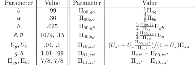
For the KS economy, the calibration is the same as in dHJJ which is only a slight modification of the original KS calibration. The calibration matches select business-cycle statistics at a quarterly frequency. Relative to the OLG calibration, households are much more patient with a discount factor of .99, capital depreciates much more slowly at .025, the productivity shocks are somewhat smaller at 1.01 and .99, and the productivity shock is not iid but has persistence Πgg= Πbb= 7/8. All the parameters including
the employment process parameters are listed in Table 2.
Parameter Value Parameter Value
β .99 Π00,gg 13Πgg
α .36 Π00,bb 35Πbb
δ .025 Π00,gb 54
Π00,bb Πbb Πgb
¯
e,u¯ 10/9, .15 Π00,bg 34ΠΠ00,gg
gg Πbg Ug, Ub .04, .1 Π10,zz0 (Uz0−Uz
Π00,zz0
Πzz0 )/(1−Uz)Πzz0
g, b 1.01, .99 Π01,zz0 Πzz0−Π00,zz0
Πgg,Πbb 7/8, 7/8 Π11,zz0 Πzz0−Π10,zz0
Table 2: KS Calibration
5
Implementation
This section discusses implementation issues specific to solving the OLG and KS economies using both the Smolyak and KS methods. In abstract, the procedure for computing equilibrium is the same across both economies and both methods. Fixing a law of motion, backward induction along with Carroll’s (2006) endogenous gridpoints method is used to solve the household problem. The household capital policies are then used to update the law of motion. This procedure is repeated until the change in the consumption policy and law of motion is less than 10−7 in levels. The rest of this section discusses the
solution procedures in more detail.
5.1
Specific Implementation for OLG
There are several implementation choices to be made when using the Smolyak method to compute the OLG economy. One pertains to representing the distribution of capital holdings. In particular, the distribution can be represented as in the theoretical model by using the levels of capital holdings across agents, k= (0, k2, . . . , kT). However, one can instead use (K,s) where srepresents the capital holding
two state spaces will result in different numerical solutions. It was found that using (K,s) produced less error in both the forecasted capital stock and in the Euler equations, and so this is adopted as the benchmark method. The appendix presents accuracy numbers for the other state space representation. The state space bounds were taken to be±20% of the (non-stochastic) steady-state capital stock and
±40% of the steady-state share distribution. In general, it is a good idea to place state space bounds as
±X% of the steady-state values as this will cluster the collocation points around the steady-state values. Another implementation choice applies only if using shares in the state space and regards handling of the restriction Ps= 1. The Smolyak algorithm is not designed to handle this case because it gives
collocation points{(K,s)} ⊂RT+1 that in general will not satisfy this restriction. The method I adopt
is to use a mapping from the hypercube [0,1]T into the unit-simplex ∆(T−1)⊂[0,1]T. In particular,
given a collocation point (K,˜s) with P
˜s6= 1, the mapping s= ˜s/P
˜sis used to recover (K,s) with
Ps = 1. For the reverse mapping,˜s= sis used. The appendix explores a different mapping that is
more uniform in a probabilistic sense but produces a worse approximation.
A final implementation choice regards simulating the economy. One can construct an approximation to the law of motion and use it to find the distribution of capital next period. Alternatively, one can construct approximations to the capital policy functions and use these to find the distribution. In solving the model, this is a non-issue because the two agree at the collocation points. It was found that approximating the capital policies produced less error, and so this is adopted in the benchmark. The appendix presents accuracy numbers for the other method.
To solve for equilibrium using the KS method, the law was updated by non-stochastically simulating the economy for 5000 periods, discarding the first 1000 periods, and using least squares regression to obtain a new law of motion (no relaxation was used).23 The grid for aggregate capital was set to cover
±60% of the steady-state capital stock with 11 evenly-spaced points. A linear rather than log-linear functional form for the law of motion was assumed but the two result in nearly identical approximations.24
5.2
Specific Implementation for KS
To solve for equilibrium in the KS economy using the Smolyak method, the following implementation was used. After choosing a set K of capital gridpoints, the infinite-dimensional distribution µ(k, s) over k ∈ [0,k¯], s ∈ {0,1} was approximated by a discrete distribution ˜µ(k, s) over k ∈ K, s ∈ {0,1}
using the method of Young (2010). The capital grid was constructed using 100 gridpoints resulting in a distribution of dimension 200. Typically the population would be normalized to unity implying the restriction P
˜
µ(k, s) = 1 in which case the collocation points would not all satisfy this restriction. However, all that matters for prices is the capital-labor ratio, and so I did not impose this.25 The bounds
on the state space were taken to be ±100% of the steady state-distribution.26 Instead of iterating to
convergence on the household problem every time before updating the law, it was found that iterating only ten times converged to arbitrary precision, did not require relaxation, and was fast (this process was repeated until both the law of motion and policies fully converged).
To solve for equilibrium using the KS method, the law was updated by non-stochastically simulating the economy for 5000 periods, discarding the first 1000 periods, and obtaining new coefficients through
23No relaxation was used for the Smolyak method either.
24The Smolyak method’s law of motion was also represented using levels so this makes for a straightforward comparison.
In section 6 I argue no functional form will result in quasi-aggregation for smallT.
25Originally the collocation points{µˆ}were mapped into the simplex using the transformation ˜µ= ˆµ/P
ˆ
µ. However, it was found that not using this mapping resulted in smaller Euler-equation errors and a more stable solution.
26This isn’t entirely true as a small constant 10−6 was added to the upper bound to ensure the hypercube had positive
least squares regression. The law was only updated after iterating to convergence on the household problem. When updating the law, a relaxation parameter of .5 was used as a looser value of .25 did not converge. The grid for aggregate capital was set to cover±30% of the steady-state capital stock using 11 evenly-spaced points. A linear functional form for the law of motion was assumed.
6
Performance
This section analyzes the performance of the Smolyak and KS methods in computing the OLG and KS economies.
6.1
OLG economy
To evaluate the accuracy of the Smolyak and KS solution methods for the OLG economy, I focus on capital-stock forecast errors and Euler-equation errors along a long simulated path. The path is simulated using the true law of motion. The simulation length is set to 15000 periods and the first 1000 periods are discarded.
To assess the accuracy of the approximate law of motion, the one-step ahead capital-stock forecasts are compared with the realized values in several ways. One measure of the accuracy is given by the largest forecast error|Kˆ0−K0|/K0 observed during the simulation where ˆK0 is the forecasted value and
K0 the actual. Another measure is the R2 statistic which indicates how much of the variation in K0 is
explained by ˆK0.27 As there is a separate approximate law of motion for each (δ, z) pair, there are four
R2 statistics and the worst of these is referred to as “minimalR2.” For the KS method, an upper bound
on the minimal R2 value is found by running a linear regression ex post on the simulated data. As a robustness check, a log-linear regression is also run to calculate the best minimal R2 were a log-linear
law of motion to be assumed for the KS method. The maximum error, minimal R2, and best-possible
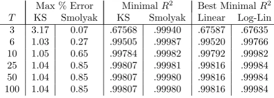
minimalR2values are reported in Table 3.
Max % Error MinimalR2 Best MinimalR2 T KS Smolyak KS Smolyak Linear Log-Lin 3 3.17 0.07 .67568 .99940 .67587 .67635 6 1.03 0.27 .99505 .99987 .99520 .99766 10 1.05 0.65 .99784 .99982 .99792 .99982 25 1.04 0.85 .99807 .99981 .99816 .99984 50 1.04 0.85 .99807 .99980 .99816 .99984 100 1.04 0.85 .99807 .99980 .99816 .99984
Table 3: Error in the Law of Motion
When the number of generations is small, the Smolyak method performs much better than the KS method. The KS method produces maximum errors as large as 3.17% and an R2 value as low as.676.
In contrast, the Smolyak method’s maximum error is only .07% and its minimal R2 statistic is .999.
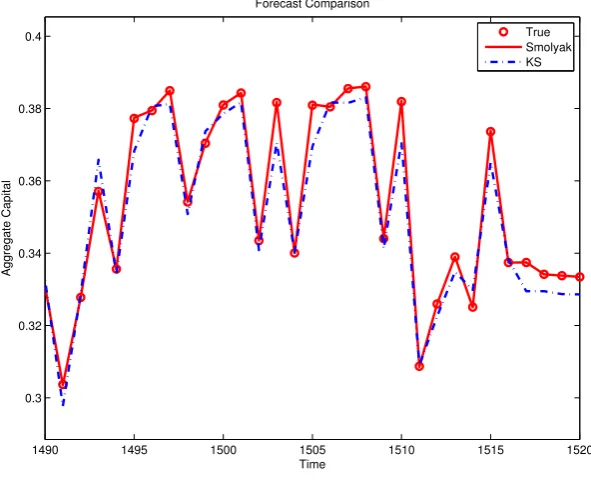
That the Smolyak method performs better in this case is confirmed visually in Figure 1 which plots the capital-stock forecasts made by both the Smolyak and KS methods with the true values. While the Smolyak forecasts and true values are virtually indistinguishable, the KS forecasts deviate noticeably.
The reason quasi-aggregation fails to obtain for small T is clear. When there are only three gen-erations, marginal propensities to save (which are roughly .54, .41 and 0 for generations 1, 2, and 3
27Formally this is computed asR2= 1−P
( ˆK0−K0)2/P
1490 1495 1500 1505 1510 1515 1520 0.3
0.32 0.34 0.36 0.38 0.4
Time
Aggregate Capital
Forecast Comparison
True Smolyak KS
Figure 1: Capital Stock Forecasts forT = 3
respectively) differ substantially. Moreover a generation’s share of total capital and labor income fluc-tuates greatly because of large depreciation shocks that only affect capital-rich generations. When the youngest generation holds most of the income, the aggregate propensity to save is roughly .54. If instead the middle-aged or oldest generation holds most of the income, the aggregate propensity to save is closer to .41 or 0 respectively. Hence what matters here is not just aggregate income (given by the capital stock), but also the share of income held by each generation which varies substantially with the history of aggregate shocks. As argued in KK, if either the marginal propensities to save were similar or the distribution did not vary much, quasi-aggregation would obtain.
Furthermore, this failure of quasi-aggregation for smallT is not due to the chosen functional form of the law of motion. This is made clear in Figure 2 where a scatter plot of today vs tomorrow’s capital stock is contrasted against the best linear rules (one for each pair of shocks) one could have. While a linear rule does not work well, this figure also demonstrates that any forecast rule that is afunction of today’s shocks and capital stock will fail to produce a good fit because the capital stock “clouds” are stacked one on another.
For a larger number of generations, the KS and Smolyak method result in similar performance. For example, when there are 100 generations, the maximum observed error is 1.04% for the KS method and 0.85% for the Smolyak method with minimalR2 values of .9981 for the KS method and .9998 for the Smolyak method. The KS method’s performance noticeably improves as T is increased, while the Smolyak method’s performance improves by one measure and worsens by another.
The reason for the KS method’s improved performance is clear. In the limiting economy as T goes large,γi, the marginal propensity to save of generationi, converges to β for any fixedi. Hence nearly
all households have nearly the same marginal propensity to save resulting in quasi-aggregation. Since quasi-aggregation obtains, the KS method performs well.
0.3 0.32 0.34 0.36 0.38 0.4 0.3
0.32 0.34 0.36 0.38 0.4
K
K’
Today vs Tomorrow’s Capital Stock
True K’ Best Linear Fit
Figure 2: Today vs Tomorrow’s Capital Stock for T = 3
by keeping track of the entire distribution, its performance is not tied to quasi-aggregation. Rather, the method’s performance hinges on the polynomial structure of the law of motion which does not fundamentally change asT increases.
To test the accuracy of the household policy functions, both maximum and average Euler-equation errors are computed along the simulated path. The errors are computed following Judd (1992) as
EEEti(ωt) = log10
1−u 0−1(β
Eu0(cit+1+1(k
i+1
t+1(k
i
t;ωt); ˆωt+1))R(ˆωt+1)) ci
t(kit;ωt)
(11)
whereR(ˆωt+1) = 1 +zt+1αKˆtα+1−1−δt+1 andu(·) = log(·). For the Smolyak method,ωt= (zt, δt, Kt,st),
ˆ
ωt+1 = (zt+1, δt+1,Kˆt+1,ˆst+1), and ( ˆKt+1,ˆst+1) is the aggregate state next period according to the
perceived law of motion. For the KS method,st and ˆst+1 are simply dropped from the definition ofωt
and ˆωt+1. The interpretation of these errors, derived from Judd and Guu (1997), is that a one-dollar
mistake in optimization is made for every 10−EEEi
t dollars spent. For example, ifEEEi
t is−3, then a
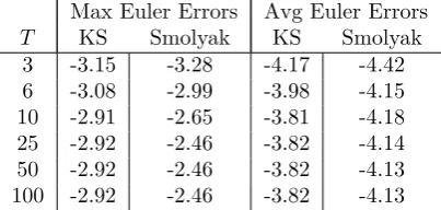
one-dollar mistake is made for every 1000 dollars spent. Note that as has typically been done in the literature the Euler errors are measured with respect to the perceived state next period. In this sense they isolate household optimization error conditional on a law of motion from error in the law of motion. Table 4 reports the maximum and average errors (across both generations and time). For the most part, the optimization errors of the two methods are comparable. Whereas the KS method results in smaller maximum errors, the Smolyak methods results in smaller average errors. For large T, the maximum percent errors for the Smolyak method are noticeably larger than those for the KS method and result in a one-dollar mistake for every 290 dollars spent compared to 830 for the KS method. The performance of both methods tends to decrease asT increases but appears to level off forT ≥25.
Max Euler Errors Avg Euler Errors
T KS Smolyak KS Smolyak 3 -3.15 -3.28 -4.17 -4.42 6 -3.08 -2.99 -3.98 -4.15 10 -2.91 -2.65 -3.81 -4.18 25 -2.92 -2.46 -3.82 -4.14 50 -2.92 -2.46 -3.82 -4.13 100 -2.92 -2.46 -3.82 -4.13
Table 4: Euler-Equation Errors in the OLG Economy
solution makes it possible to see why this is the case. The chosen implementation of the Smolyak method effectively constructs an approximation of the function
ki+1,ki,z,δ(K,s) =γi(1 +zαKα−1−δ)ki (12) for eachi >1,kiin a grid, and (z, δ) combination (i= 1 is similar). Becauseαis in (0,1), this function is not a polynomial. Hence, away from the collocation points the approximation is not perfect. However, note that this is a function of only one variable, K, and that the polynomial basis used has terms K
and K2. Because of this, the approximation is quite good for any generation and any level of capital
holdings.
It is also possible to see what indexing the policy functions and separating the individual from the aggregate state accomplishes. If the policy function were not indexed, then the Smolyak approximation would be applied to
ki+1,z,δ(ki;K,s) =γi(1 +zαKα−1−δ)ki (13) which has a termkiand a cross termkiKα−1. To capture the impact of this cross term, one would need a finer Smolyak approximation. If in addition the aggregate and individual states were combined, the Smolyak approximation would be applied to
ki+1,z,δ(K,s) =γi(1 +zαKα−1−δ)siKT (14)
which has cross terms siK and siKα. This also would require a higher level of approximation.
Index-ing policy functions and separatIndex-ing the individual and aggregate states makes a fairly coarse Smolyak approximation accurate.
T KS Smolyak 3 0.12 .004 6 0.20 0.02 10 0.25 0.05 25 0.59 0.29 50 1.21 1.18 100 2.29 4.97
Table 5: Running Times in Minutes for the OLG Economy
6.2
KS economy
Because the KS economy does not have an analytic solution, it is difficult to assess the accuracy of the KS and Smolyak methods. This is especially true for the Smolyak method. To test the law of motion, researchers have typically compared simulated series generated using only household policies with series generated using an approximate law of motion. This is not really applicable to the Smolyak method: if the law of motion is not explicitly approximated but rather given implicitly by the policy functions, then there is no disagreement between the series. In other words, the Smolyak method has anR2 of 1
in this case. However, that does not mean there is no error in the law of motion because interpolating the policies is not typically an error-free process.
In light of this the accuracy of the Smolyak method is assessed in three ways. The first is to compute Euler-equation errors with respect to therealized aggregate state next period rather than theperceived
aggregate state. This measure gives an idea of how much error in the law of motion translates into error in household optimization. The second is to compare the capital-stock series from the Smolyak and KS simulations. In addition to the convincing argument made by KS that their computed equilibrium must be close to the true equilibrium, many different solution methods have computed nearly the same equilibrium as the KS method (cf. den Haan 2010). Hence the KS method’s solution can be used as an accuracy check. The third and final test is the comparison of a simulated series generated by explicitly approximating the capital policies with a simulated series generated by explicitly approximating the law of motion. Because it is possible to simulate the economy with either approximation, this may be helpful in assessing how well the Smolyak method is working.28 These three tests are conducted using a
simulation length of 5000 periods with the first 1000 periods discarded. The accuracy of the KS method is assessed with the first test and also the typical comparison of the forecasted and realized capital-stock sequences.
First, Euler-equation errors are computed along the simulated path and both the maximum and average errors reported. The Euler errors are calculated analogously to (11) except that the rental rate and consumption next period are found using the realized next-period moment or distribution and the errors are only counted if the capital choice is strictly positive.29 The errors for the Smolyak method are slightly smaller in both maximum and average terms but in this measure the KS and Smolyak methods are roughly equivalent.
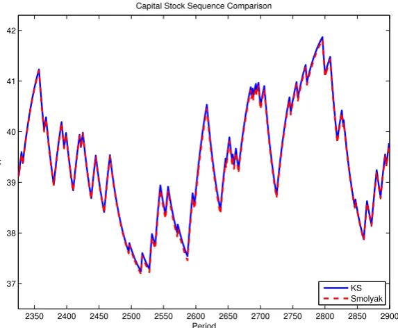
Second, the capital sequence generated by the KS method is compared with that of the Smolyak method. Table 7 reports the maximum and average differences between the Smolyak and KS aggregate capital series and Figure 3 plots them. Visually the series are almost indistinguishable although at
28This is not sure to be helpful however because the capital policies and law of motion have different properties. For
instance, typically the law of motion will vary with the distribution even if the capital policy does not. In this case it would be better to approximate the capital policies and compute the law of motion indirectly.
29When the capital choice equals zero, the no-borrowing constraint is almost certainly binding in which case the
Max Euler Errors Avg Euler Errors KS Smolyak KS Smolyak -1.89 -2.22 -4.79 -4.97
Table 6: Euler-Equation Errors in the KS Economy
times the Smolyak series lies slightly below the KS one. Over the entire simulation the series exhibit a maximum difference of only 0.28% and an average difference of 0.14%. However, while this difference is small, it is systematic with the averagenon-absolutedifference also being 0.14% (measured using the Smolyak series subtracted from the KS series) confirming what was noticed visually. As the KS method is likely very close to the truth, the proximity of these two series confirms the accuracy of the Smolyak method for this economy.
2350 2400 2450 2500 2550 2600 2650 2700 2750 2800 2850 2900 37
38 39 40 41 42
Period
K
Capital Stock Sequence Comparison
KS Smolyak
Figure 3: Simulated Capital Sequence Comparison
Max Abs (%) Mean Abs (%) Mean (%) (KS-Smolyak) 0.278 0.141 0.141
Table 7: Simulated Capital Sequence Comparison
1-Step Forecast 25-Step Forecast 100-Step Forecast KS Smolyak KS Smolyak KS Smolyak
R2 .999999 .999998 .999780 .999918 .999474 .999888 Max Abs (%) .0073 .0204 .1007 .1533 .1530 .1882 Avg Abs (%) .0021 .0026 .0346 .0454 .0554 .0769 Avg (%) -.0013 .0026 -.0211 .0454 -.0349 .0769
Table 8: Law of Motion Forecast Errors in the KS Economy
forecasts as seen in the mean absolute errors being the same as the mean errors. While the KS method is guaranteed to be correct on average (because it makes unbiased forecasts by construction), the Smolyak method is guaranteed to be correct only as the level of approximation goes large. It appears however that the lowest level of approximation produces small errors in the KS economy just as it does in the OLG economy.
Since the Smolyak method places no restrictions on the functional form of the law of motion and appears to be accurate, it is interesting to ask whether the Smolyak-approximated economy exhibits quasi-aggregation. I test this by running linear and log-linear regressionsex post on the simulated capital stock series from the Smolyak method. As should have been expected, the fit is extremely good with all theR2 values exceeding .999999. This verifies directly, inasmuch as the Smolyak solution approximates
the truth, that KS’s argument for quasi-aggregation was indeed correct: only the mean matters for this model.
The running times of the two methods are now briefly considered. While the KS method (paired with Carroll’s 2006 endogenous gridpoints method) is very fast at 3.25 minutes, the Smolyak method is also quite fast at 6.37 minutes. The Smolyak method performs quite well in this regard as it has 401 collocation points compared to the KS method’s 11 moment gridpoints. Its comparative advantage lies in avoiding the simulation step where much of the computation time is spent for the KS method.
7
Conclusion
The Smolyak method is a promising technique for computing equilibrium in dynamic heterogeneous-agent economies. While including a distribution as a state variable massively increases the dimensionality of the state space, the Smolyak sparse-grid interpolation algorithm makes this increase manageable. This technique developed in Smolyak (1963) and Barthelmann et al. (2000) shows great promise for economic applications as Krueger and Kubler (2004) first illustrated. The application of the Smolyak algorithm here results not only in tractability, but also in very good accuracy. In the KS economy the Smolyak method produces errors similar to those of the KS method. In the OLG economy, the Smolyak method performs much better than the KS method when the number of generations is small because it does not rely on quasi-aggregation which fails in this case. Moreover, for models where the distribution is finite dimensional, like in the OLG model, the method can be regarded as solving for a full rational-expectations equilibrium. In models where the distribution is infinite-dimensional, like in the KS model, the method comes very close to a full rational-expectations equilibrium.
predefined points define an interpolating function. With regards to speed, this paper has shown the Smolyak method need not be much slower than the KS method. For models with larger aggregate state spaces or where Carroll’s (2006) efficient solution method cannot be used, parallelization (which has not been used in this paper) could prove very helpful as the work by Aldrich et al. (2011) has shown.
While the application of the Smolyak algorithm here has been to approximating full-rationality equilibrium as closely as possible, the Smolyak algorithm could also be useful in solving for bounded-rationality equilibrium quickly and accurately. While many methods could benefit from the Smolyak algorithm, of particular promise is the explicit aggregation technique of den Haan and Rendahl (2010). This method avoids the simulation step of the KS method by explicitly aggregating “auxiliary” policy functions. In its most basic implementation, the auxiliary policy functions are constructed to be linear in asset holdings but as close as possible to the original policies. Because the auxiliary policies are lin-ear, they aggregate perfectly and the minimal aggregate state space is average capital holdings for each type of agent. Having more types of agents or more curvature in the auxiliary policy functions requires having more moments, but Smolyak interpolation is well adapted to handling this increase in aggregate moments. This pairing of den Haan and Rendahl’s (2010) method with the Smolyak algorithm could achieve some of the benefits of the Smolyak method (no simulation, high accuracy) while being extremely efficient. The exploration of this idea is left for future research.
References
[1] Aldrich, E., Fern´andez-Villaverde, J., Gallant, A. R., and Rubio-Ram´ırez, J. (2011), “Tapping the Supercomputer Under Your Desk: Solving Dynamic Equilibrium Models with Graphics Processors”,
Journal of Economic Dynamics and Control, 35(3), 386-393.
[2] Aruoba, S., Fern´andez-Villaverde, J., and Rubio-Ram´ırez, J. (2006) “Comparing Solution Methods for Dynamic Equilibrium Economies,” Journal of Economic Dynamics and Control, 30(12), pp. 2477-2508.
[3] Azzimonti, M., de Francisco, E., and Krusell, P. (2006) “Median-voter Equilibria in the Neoclassical Growth Model under Aggregation,”Scandinavian Journal of Economics, 108(4), pp. 587-606.
[4] Barthelmann, V., Novak, E., and Ritter, K. (2000) “High Dimensional Polynomial Interpolation on Sparse Grids,”Advances in Computational Mathematics, 12, pp. 273-288.
[5] Carroll, C. (2006) “The Method of Endogenous Gridpoints for Solving Dynamic Stochastic Opti-mization Problems,”Economics Letters, 91(3), pp. 312-320.
[6] Chien, Y., Cole, H., and Lustig, H. (2009) “A Multiplier Approach to Understanding the Macro Implications of Household Finance,” mimeo.
[7] Den Haan, W. J. (2010) “Comparison of Solutions to the Incomplete Markets Model with Aggregate Uncertainty,”Journal of Economic Dynamics and Control, 34(1), pp. 4-27.
[9] Den Haan, W. J. and Rendahl, P. (2010) “Solving the Incomplete Markets Model with Aggregate Uncertainty Using Explicit Aggregation,” Journal of Economic Dynamics and Control, 34(1), pp. 69-78.
[10] Huffman, G. (1987) “A Dynamic Equilibrium Model of Asset Prices and Transaction Volume,”
Journal of Political Economy, 95(1), pp. 138-159.
[11] Judd, K. L. (1992) “Projection Methods for Solving Aggregate Growth Models,” Journal of Eco-nomic Theory, 58(2), pp.410-452.
[12] Judd, K. L. (1998) “Numerical Methods in Economics,”MIT Press, Cambridge.
[13] Judd, K. L. and Guu, S. (1997) “Asymptotic Methods for Aggregate Growth Models,”Journal of Economic Dynamics and Control, 21(6), pp. 1025-1042.
[14] Judd, K. L., Maliar, L., and Maliar, S. (2010) “A Cluster-Grid Projection Method: Solving Problems with High-Dimensionality,” mimeo.
[15] Krueger, D. and Kubler, F. (2004) “Computing Equilibrium in OLG models with Stochastic Pro-duction,”Journal of Economic Dynamics and Control, 28(7), pp. 1411-1436.
[16] Krueger, D., Kubler, F., and Malin, B. (2011) “Computing Stochastic Dynamic Economic Models with a Large Number of State Variables: A Description and Application of a Smolyak-Collocation Method,”Journal of Economic Dynamics and Control, forthcoming.
[17] Krusell, P. and R´ıos-Rull, J.-V. (1999) “On the Size of U.S. Government: Political Economy in the Neoclassical Growth Model,”American Economic Review, 89(5), pp. 1156-1181.
[18] Krusell, P. and Smith, A. Jr. (1997) “Income and Wealth Heterogeneity, Portfolio Choice, and Equilibrium Asset Returns,”Macroeconomic Dynamics, 1(02), pp. 387-422.
[19] Krusell, P. and Smith, A. Jr. (1998) “Income and Wealth Heterogeneity in the Macroeconomy,”
Journal of Political Economy, 106(5), pp. 867-896.
[20] Reiter, M. (2010) “Solving the Incomplete Markets Model with Aggregate Uncertainty by Backward Induction,”Journal of Economic Dynamics and Control, 34(1), pp. 28-35.
[21] R´ıos-Rull, J.-V., (1997) “Computation of Equilibria in Heterogeneous Agent Models.” Federal Re-serve Bank of Minneapolis Staff Report, 231, pp. 238-264.
[22] Smolyak, S. (1963) “Quadrature and Interpolation Formulas for Tensor Products of Certain Classes of Functions,”Soviet Mathematics, Doklady, 4, pp. 240-243.
Appendix
This appendix explores alternative implementations of the Smolyak method in the context of the OLG economy (which has a known solution). Four different implementations are considered and their descrip-tions are given below.
Sm1 – Benchmark Implementation
The state space uses sharess; the mapping from ˜sin the cube to sin the simplex is s= ˜s/P˜sand the
reverse mapping is ˜s=s; and the distribution is forecasted using an approximated capital policy function (not an approximate law of motion). Because of the loss in dimension in mapping to the simplex, there are many reverse mappings into the cube.30
Sm2 – Alternative Mapping
The state space uses sharess; the mapping from ˜sin the cube tosin the simplex iss=−log(˜s)/P−log(˜s)
and the reverse mapping is ˜s=e(10 log(.5)s); and the distribution is forecasted using approximated policy functions. The mapping is motivated by a method of drawing uniformly from a unit simplex (which is accomplished by drawing from the Dirichlet distribution with concentration parameter equal to 1). Several reverse mappings were tried, but the one used worked best.31
Sm3 – Simpler State Space
The state space uses levels of capital stock for each generationk; there is no mapping; and the distribution is forecasted using an approximated capital policy function.
Sm4 – Simpler State Space, Alternative Simulation Method
The state space uses levels of capital stock for each generationk; there is no mapping; and the distribution is forecasted using an approximated law of motion.
The accuracy numbers for the laws of motion are displayed in Table 9. For space, theR2values are
rounded to three decimal places. Alternative implementations of the Smolyak method display similar characteristics to the benchmark implementation: each outperforms the KS method for smallT (which is when quasi-aggregation breaks down) and the performance of each implementation decreases as the number of periods increases. Sm1 and Sm2 display similar errors which are less than the errors of Sm3 and Sm4. This suggests that the precise mapping of shares may not matter as much as the choice of whether or not to use shares. That Sm1 and Sm2 perform better than Sm3 and Sm4 is likely due to the ability of Smolyak interpolation to achieve high accuracy in one dimension relative to accuracy in several dimension as discussed in the main text. Because Sm1 and Sm2 includeK in the state space directly rather than indirectly throughK=P
k/T, Sm1 and Sm2 exploit this feature of the Smolyak algorithm and so capture more of the general equilibrium effects.
30It’s unclear which of these reverse mappings is optimal, but the identity mapping is a natural choice.
31In some sense, the reverse mapping ˜s=e(Tlog(.5)s) should be optimal because most of the time,P
Max % Error Minimal R2
T KS Sm1 Sm2 Sm3 Sm4 KS Sm1 Sm2 Sm3 Sm4 3 3.17 0.07 0.07 0.22 0.37 .676 .999 .999 .997 .996 6 1.03 0.27 0.27 0.84 1.25 .995 1.000 1.000 .996 .992 10 1.05 0.65 0.66 1.42 1.85 .998 1.000 1.000 .995 .989 25 1.04 0.85 0.86 1.66 2.14 .998 1.000 1.000 .994 .987 50 1.04 0.85 0.86 1.66 2.14 .998 1.000 1.000 .994 .987 100 1.04 0.85 0.86 1.66 2.14 .998 1.000 1.000 .994 .987
Table 9: Accuracy of the Law of Motion
The Euler equation errors are reported in Table 10. Again, the alternative implementations display similar patterns to the benchmark one: the errors are smaller than the KS method errors forT = 3 but increase in the number of generations. Again, Sm1 and Sm2 fair better than Sm3 and Sm4, with Sm1 outperforming Sm2 most of the time. While the KS method tends to produce less error, the errors of the Smolyak implementations would not typically be considered large, at least in terms of average errors. Note that Sm3 and Sm4 have the exact same solution but different simulations (and so result in different maximum and average errors along the simulation path).
Max Euler Errors Avg Euler Errors
T KS Sm1 Sm2 Sm3 Sm4 KS Sm1 Sm2 Sm3 Sm4 3 -3.15 -3.28 -3.28 -3.27 -3.27 -4.17 -4.42 -4.41 -4.19 -4.16 6 -3.08 -2.99 -3.05 -2.24 -2.14 -3.98 -4.15 -4.11 -3.25 -3.27 10 -2.91 -2.65 -2.24 -1.94 -1.82 -3.81 -4.18 -3.71 -3.06 -3.08 25 -2.92 -2.46 -2.12 -1.86 -1.72 -3.82 -4.14 -3.73 -3.01 -3.03 50 -2.92 -2.46 -2.20 -1.86 -1.72 -3.82 -4.13 -3.82 -3.01 -3.03 100 -2.92 -2.46 -2.28 -1.86 -1.72 -3.82 -4.13 -3.92 -3.01 -3.03
Table 10: Accuracy of the Policy Functions
The running times for the various implementations are reported in Table 11. As running times are virtually the same for Sm1 as Sm2 and Sm3 as Sm4, I only report joint Sm1/Sm2 and Sm3/Sm4 times. The Sm3 and Sm4 implementations take slightly longer to run than the Sm1 and Sm2 implementations. This is not because the actual interpolation takes any longer but because extra iterations required for the law of motion to converge, which is itself due to larger errors in the law of motion.
T KS Sm1/Sm2 Sm3/Sm4 3 0.12 0.00 0.00 6 0.20 0.02 0.02 10 0.25 0.05 0.05 25 0.59 0.29 0.34 50 1.21 1.18 1.40 100 2.29 4.97 6.00