ABSTRACT
KUO, CHUN-HUNG. Three Essays on Macroeconometrics. (Under the direction of Atsushi Inoue.)
Chapter 1 discusses the overview of the dissertaion and highlight the importance of model
misspecification issues in DSGE models. Methodology of approaching these issues is compactly
discussed.
Chapter 2 proposes a new algorithm for solving computationally challenging heterogeneous
agent (HA) models. The algorithm combines the value function iteration (VFI) method, the
endogenous grid points method (EGM), and the explicit aggregation (XPA) method. This new
algorithm is robust in the sense that the initial values are irrelevant for finding the optimal policy
functions. Moreover, it is also fast because both the root-finding procedure for the household
problem and the repeated simulation for the aggregate law of motion are not necessary. The
algorithm solves a typical HA model within just a few seconds on a ordinary desktop computer.
As a consequence, it could be a proper tool for structural estimation of HA models, which needs
to solve the model several thousands times.
Currently, heterogeneous agent (HA) models still rely on calibration for model parameters,
which makes the quantitative implications of these models shaky. Since HA models can trace
both the dynamics of the cross-sectional consumption (and/or wealth) distributions and those
of aggregate variables, a HA model is estimated by utilizing two sources of data: the first one is
repeated cross-sectional data from the Consumer Expenditure Surveys (CEX), and the second
one is the aggregate data from the National Income and Production Accounts (NIPA) of the
United States. In particular, the Laplace-type estimator (LTE) with criterion function from
indirect inference is adopted. Therefore, the daunting global optimization task is replaced by
the Markov Chain Monte Carlo method. Therefore, Chapter 3 is methodologically oriented, and
focuses on proposing a recipe for conducting the structural estimation of HA models, a task
In Chapter 4 we consider a dynamic stochastic general equilibrium (DSGE) model with
distortions. Our framework allows us to analyze the quantitative importance of model
misspec-ification and identify the location of model misspecmisspec-ification. To illustrate our framework, we
estimate a New Keynesian DSGE model with distortions using US macroeconomic time series.
We find that the DSGE model is largely misspecified, especially in the labor market.
Specifi-cally, the forecast error variance decomposition (FEVD) exercise reveals that, for all aggregate
variables used to estimate the model, the labor market misspecification contributes to more
©Copyright 2012 by Chun-Hung Kuo
Three Essays on Macroeconometrics
by Chun-Hung Kuo
A dissertation submitted to the Graduate Faculty of North Carolina State University
in partial fulfillment of the requirements for the Degree of
Doctor of Philosophy
Economics
Raleigh, North Carolina
2012
APPROVED BY:
Douglas K. Pearce Moody T. Chu
Nora Traum Atsushi Inoue
DEDICATION
BIOGRAPHY
Chun-Hung Kuo is a PhD candidate at North Carolina State University. His main research
area is applied econometrics and macroeconomics with focus on structural estimation, model
misspecification, and related computational methods. He is also interested in wealth and income
inequality, and numerical methods for solving dynamic stochastic general equilibrium (DSGE)
ACKNOWLEDGEMENTS
First and foremost, I would like to thank my dissertation advisor, Dr. Atsushi Inoue, for his
support, patience, and helpful criticism. I would not have been able to complete this dissertation
without his step-by-step guidance. I would also like to thank Dr. Moody Chu for sharing his
knowledge on numerical analysis. His continuous encouragement enabled me to put myself in a
position to finish my dissertation. I would like to express my gratitude to Dr. Pablo Guerron for
leading me into the world of dynamic macroeconomics. I am grateful towards Dr. Barbara Rossi
for giving me the opportunity to work on a National Science Foundation project as one of my
dissertation chapters. I would like to thank Dr. Douglas Pearce and Dr. Nora Traum for their
valuable comments that improved my dissertation. At last, I would like to thank my graduate
school colleagues, including Steve Tsang, Chien-Yu Huang, Timothy Hamilton, Robert Kane,
TABLE OF CONTENTS
List of Tables . . . vii
List of Figures . . . .viii
Chapter 1 Overview of the Dissertation. . . 1
1.1 Motivation . . . 1
1.2 The Methodology . . . 3
Chapter 2 A New Algorithm for Solving Heterogeneous Agents Models . . . . 6
2.1 Introduction . . . 6
2.2 Literature for Algorithms . . . 8
2.3 A Heterogeneous Agents Model . . . 10
2.3.1 Model Setting . . . 11
2.3.2 Recursive Competitive Equilibrium . . . 13
2.4 The Algorithm . . . 17
2.4.1 Housekeeping . . . 17
2.4.2 Implementation of the Algorithm . . . 18
2.5 Numerical Results . . . 21
2.5.1 Calibration . . . 21
2.5.2 Some Preliminary Results . . . 22
2.5.3 Comparison with Existing Algorithms . . . 25
2.6 Conclusion . . . 28
Chapter 3 Estimation of Heterogeneous Agent Models . . . 29
3.1 Introduction . . . 29
3.2 Literature Review . . . 32
3.2.1 Review of Heterogeneous Agent Models . . . 32
3.2.2 Review of Empirical Studies . . . 33
3.2.3 Review of Estimation Methods . . . 35
3.3 The Model . . . 37
3.4 Empirical Methodology . . . 41
3.4.1 Some Technical Necessaries . . . 41
3.4.2 The Estimation Strategy . . . 44
3.5 The Data . . . 46
3.5.1 NIPA Data . . . 46
3.5.2 CEX Data . . . 47
3.6 Empirical Results . . . 49
3.7 Conclusion . . . 51
Chapter 4 Identifying Sources of Misspecification in DSGE Models . . . 52
4.1 Introduction . . . 52
4.2.1 The Final Good Firm Problem . . . 56
4.2.2 The Intermediate Good Firm Problem . . . 57
4.2.3 The Household Problem . . . 62
4.2.4 Aggregation Issues . . . 68
4.2.5 Government Policy . . . 70
4.3 Empirical Methodology . . . 70
4.3.1 The Data . . . 70
4.3.2 Bayesian Inference . . . 71
4.3.3 Prior Settings . . . 72
4.4 Empirical Results . . . 78
4.4.1 Parameter Estimates . . . 78
4.4.2 Impulse Response Functions . . . 80
4.4.3 Forecast Error Variance Decompositions (FEVD) . . . 84
4.5 Simulation Exercises . . . 85
4.5.1 The Model . . . 87
4.5.2 Misspecified Models . . . 93
4.5.3 The Empirical Strategy and Results . . . 94
4.6 Conclusion . . . 97
References. . . 98
Appendices . . . .104
Appendix A Recursive Competitive Equilibrium (RCE) . . . 105
Appendix B Equilibrium Conditions . . . 107
B.1 Aggregation . . . 107
B.2 Steady State . . . 110
B.3 Linearized Equilibrium Conditions . . . 111
LIST OF TABLES
Table 2.1 Parameters Calibration . . . 22
Table 2.2 The Euler Equation Residuals . . . 25
Table 2.3 Computation Time . . . 28
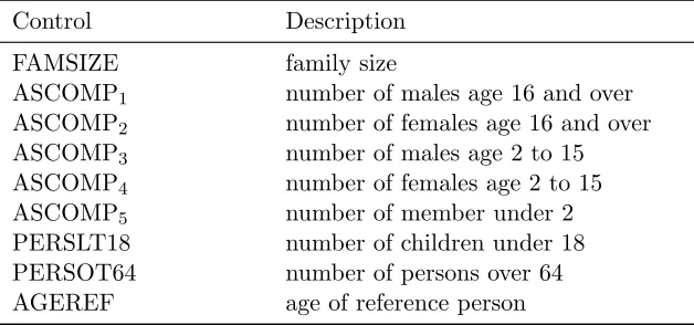
Table 3.1 Meaning of Control Variables . . . 49
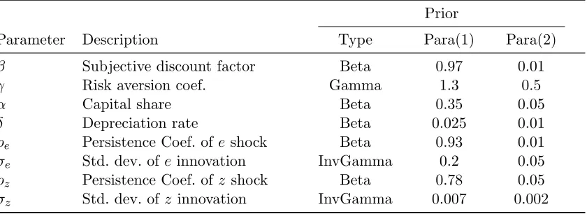
Table 3.2 Prior Distributions of Structural Parameters . . . 50
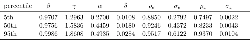
Table 3.3 Posterior of Structural Parameters . . . 51
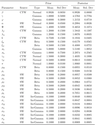
Table 4.1 Prior and Posterior for the Benchmark Case . . . 76
Table 4.2 Priors and Posteriors: Restricted Case . . . 77
Table 4.3 Variance Decomposition: Real GDP . . . 85
Table 4.4 Variance Decomposition: Real Consumption . . . 85
Table 4.5 Variance Decomposition: Real Investment . . . 85
Table 4.6 Variance Decomposition: Hours Worked . . . 86
Table 4.7 Variance Decomposition: (Quarterly) Inflation Rate . . . 86
Table 4.8 Variance Decomposition: Real Wage Rate . . . 86
Table 4.9 Variance Decomposition: (Quarterly) Federal Fund Rate . . . 86
Table 4.10 DGP and prior distributions . . . 95
LIST OF FIGURES
Figure 2.1 Individual Policy Functions of the Benchmark Calibration . . . 23
Figure 2.2 Simulated Value of Aggregate Capital of Benchmark Calibration . . . 24
Figure 4.1 Impulse Response Functions (Monetary Policy Shock) . . . 81
Chapter 1
Overview of the Dissertation
1.1
Motivation
In this chapter, I provide an overview of my dissertation. Broadly speaking, the dissertation is
about issues of model misspecification in the context of Dynamics Stochastic General
Equilib-rium (DSGE) models.
For an empirical economist, the first challenge facing her is usually model specification,
before she conducts her econometric analysis. Often she has to answer followings questions:
whether some important explanatory variables are excluded, whether the functional form of the
regression model is appropriate, whether the assumption about the error term is reasonable,
etc. Only when can she properly answer the above questions, her reader start to consider
her empirical studies seriously. If she has a dubious model specification but adopts a fancy
estimation method, the value of the empirical studies will still be limited. I do not mean that
the choice of estimation method is not important; I merely want to to emphasize that the
priority of model misspecification is higher than the estimation methods.
Econometricians recognize the consequences of adopting misspecified models, and they have
studied the widely, especially in reduced-form regression models. However, studies about model
of the issue. Different from traditional reduced-form regression models, the structure of DSGE
models is complex. DSGE models might contains dozens of non-linear equations and endogenous
variables as well as several exogenous shocks. Their complicated structures make the theoretical
econometric investigation difficult, if not impossible.
After three decades’ development, economists have invented many DSGE models. One of
main reasons of inventing DSGE model is to provide explanation for various economic
phenom-ena. Broadly speaking, when a economist constructs a new model to explain certain aspects of
the data, she is providing a new model specification. If the new model can explain that
partic-ular aspect of the data, the economist tends to claim that the new model is better than the old
one, and suggests, at least implicitly, that the old model should be discarded. This procedure is
apt for choosing a better model, if the sole goal of research is providing economic explanation.
However, economists construct their models not just for positive analysis (e.g. what causes
the high risk premium). We can also use DSGE model for normative analysis (e.g. asking what
the optimal monetary policy is) as well as for economic forecast. Under these circumstances,
the procedure helps less, since we just want to use the model. In contrast, understanding the
shortcoming of the model at hand is informative for the user of the model. I do not intend
to discredit above procedure for selecting a better model. I just mean that understanding the
limitation of a considered model is informative for some purposes.
As Woodford (2009) argues, both the New classical and the New Keynesian economists now
embrace DSGE models, and the DSGE models have become the standard framework for
macroe-conomic studies. A common feature of existing studies using DSGE models is that economists
seek for not only qualitative but also quantitative implications. The requirement for
quantita-tive implications makes parameter estimation inevitable. Along with the rapid development of
DSGE models, econometricians have proposed various estimation methods for DSGE models.
The existing methods for estimating DSGE models consist of the Generalized Method of
Mo-ment (GMM), the Maximum Likelihood Estimation (MLE) method, the Bayesian estimation
Now many empirical studies are based the estimated DSGE models such as Christiano
et al. (2005), Smets and Wouters (2007), and Justiniano and Primiceri (2008), just name a few.
However, to best of my knowledge, when estimating DSGE models, economists have not yet
tackled the obvious model misspecification due to the representative agent (RA) assumption.
The main justification of the RA assumption is that individuals can fully insure their risks.
That is, the markets should be complete. Unfortunately, complete markets are usually rejected
in empirical studies. For example, see Cochrane (1991) and Attanasio and Browning (1995).
Since RA setting is hard to justify, a serious treatment on model misspecification due to the
RA assumption is necessary.
Therefore, in this dissertation I would like to deal with two model misspecification issues
in DSGE models. First, I deal with misspecification due to the RA assumption, and estimate
the structural parameters of a HA model. Second, I propose a framework for identifying the
sources of model misspecification in DSGE models.
1.2
The Methodology
To deal with the two misspecification problem raised in the previous section, several
econo-metrics methods are used in the dissertation. I briefly discuss my methodology of using these
econometric methods in the dissertation in turn.
When economists estimate RA models, they often rely on likelihood-function-based
meth-ods. For example, McGrattan et al. (1997), and Ireland (2001) use MLE, and Smets and Wouters
(2007) use the Bayesian estimation method. However, economists still do not know how to
express HA models to the state space form, and thus we cannot adopt the
likelihood-function-based methods (i.e., MLE and Bayesian method). Moreover, we cannot use GMM to estimate
a HA model as well, because the first order conditions of HA models contain both aggregate
and individual variables. It is not straightforward to use them together for estimation.
To achieve the goal of estimating a HA model, I combine two estimation methods that
main idea of Indirect Inference is to use an auxiliary model to capture the important aspects
of observed data. If one can simulate the structural model, then one can also use the simulated
data to obtain auxiliary parameter estimates. Indirect Inference chooses structural parameters
in such a way that the estimated auxiliary parameters from both observed and simulated data
are as close as possible. Indirect Inference is particular useful when the likelihood function of
the data is not tractable. It is exactly the situation that we are facing.
The reason of introducing LTE is to overcome the difficulty coming from global optimization
problem, if we solely use the Indirect Inference. Chernozhukov and Hong (2003) show that
LTE has a computational advantage in dealing with cases where the criterion functions have
multiple local modes or are highly non-convex, while the global optimum are well defined. The
logic of LTE is to transform a criterion function to a well-defined density function by a Laplace
type transformation. The criterion function does not have to be a likelihood function. In my
implementation, the needed criterion function stems from indirect inference. Once the deduced
density function, or quasi-posterior function, is obtained, we can use the standard Markov
Chain Monte Carlo (MCMC) method to conduct random draws with respect to it. Besides, to
implement the above hybrid estimation method, I need a algorithm to solve the HA model. I
do not use the existing algorithms. Rather, I propose a new algorithm that is fast and robust.
Please refer to the next chapter for the detail of the algorithm.
As I explained in previous the section, knowing the limitation of a models is useful for the
user of models. However, macroeconomists are often left to wonder if their models are
misspeci-fied and, if they are, what parts of models are misspecimisspeci-fied, even though model misspecification
may be widespread. I propose an empirical framework for this issue. The framework is easy
to use, and only the Bayesian estimation method is involved. To illustrate the framework, I
consider a New Keynesian DSGE model based on Christiano, Eichenbaum and Evans (2005)
and Smets and Wouters (2007). The model is mildly misspecified in the sense that (i) the cross
equation and equilibrium restrictions imposed by the model do not exactly hold in every time
model (both firms and households) take into account exogenous stochastic processes of
devia-tions when they solve their optimization problems. The variances of deviadevia-tions are a measure
of the degree of misspecification of the New Keynesian DSGE model without a distortion.
After estimating the parameters of the models as well as those of deviation processes, I
conduct forecast error variance decompositions (FEVD) to locate possible sources of
misspec-ification. This method is closed related to Chari et al. (2007) who also introduce time-varying
“wedges” into a macroeconomic model. There are two main differences. One difference is that
they consider a stochastic growth model with wedges (what they call the benchmark prototype
economy) while we consider a New Keynesian DSGE model with wedges. Our New Keynesian
DSGE model is based on Christiano, Eichenbaum and Evans (2005) and Smets and Wouters
(2007) and incorporates frictions. Thus the distortions reflect model misspecification that
can-not be accounted for by the built-in frictions. The other difference is that their analysis is based
on calibrating parameter values while mine is based on estimated parameters that take into
Chapter 2
A New Algorithm for Solving
Heterogeneous Agents Models
2.1
Introduction
In the literature, many algorithms have already been proposed to solve heterogeneous agent
models. Each of them has its own limitations in terms of computation time, numerical
insta-bilities for different parameter combinations, or difficulties in coding. In this chapter, I take
these limitations into account and provide a new algorithm that drastically improves the speed
and reliability for solving heterogeneous agent models. More importantly, this new algorithm is
particularly useful for structural estimation of heterogeneous agent models. The algorithm has
three key components: Value Function Iteration (hereafter, VFI), 1 Endogenous Grid points method (hereafter, EGM) of Carroll (2006), and explicit aggregation (hereafter, Xpa) of den
Haan and Rendahl (2010).
The basic idea of VFI is follows. One makes an initial guess of the value function of the
problem. With the initial guess, one solves the right hand side of the Bellman equation and
updates the value function until it converges. The main strength of VFI is that it relies on the
1
contraction mapping theorem and, hence, possesses excellent convergence properties. In
con-trast, Euler-equation-based methods, which rely on the first-order conditions of the recursive
problems to find the solution, cannot assure convergence unless one has good initial
conjec-tures for the solution. Moreover, VFI is suitable to handle the problems with discontinuities
or nondifferentiabilities problems coming from borrowing limits and discrete choices.
Euler-equation-based methods usually run into difficulties in these situations. The main drawback of
VFI is its speed, and it suffers from a strong case of the curse of dimensionality when the the
dimensions of state space increase. In the literature, there are many variants of VFI, including
discretized VFI, parametrized VFI, or VFI with interpolation. The differences between them
are the methods used to keep the information of the value function. Heer and Maussner (2009)
give very detail explanations for different versions of value function iteration.
The EGM of Carroll (2006) is an important contribution on solving dynamic economic
models.2This method changes the time convention of state variables and, by doing so, prevents the intensive computation of the root-finding procedure, which is the most time-consuming
part of VFI. Details of the algorithm will be discussed in Section 2.4. By including the idea
of EGM, VFI becomes a very attractive algorithm, because one can enjoy the strength of
both algorithms, i.e., the convergence property of VFI and the speed improvement of EGM.
Barillas and Fernandez-Villaverde (2007) demonstrate how to combine these two algorithms
using stochastic neoclassical growth models as examples.
Finally, by including the methodology of Xpa, the new algorithm can obtain the aggregate
law of motion of the model by a simple weighted average. Xpa helps one prevent the simulation
step of the Krusell-Smith algorithm, which is computationally expensive and prone to numerical
instabilities. The combination of VFI, EGM and Xpa makes the new algorithm a reliable and fast
tool for solving heterogeneous agent models. In fact, it solves the heterogeneous agent models
in just a few seconds. Section 2.2 provides a brief comparison between the new algorithm and
existing ones.
2
2.2
Literature for Algorithms
Krusell and Smith (1998) remains the standard algorithm for solving heterogeneous agent
mod-els.3The goal of Krusell and Smith (1998) is to find an aggregate law of motion for the aggregate variable that is consistent with the decision on individual capital accumulation. To accomplish
this, one needs to first guess an aggregate law of motion in some parametric way. Given this
conjecture on the aggregate law of motion, one then solves the individual recursive problem to
obtain the policy functions. Next, one uses the deduced policy functions to simulate an
econ-omy with a large number of individuals. Not surprisingly, this is done by taking into account
both idiosyncratic and aggregate shocks. By simulating the economy this way, the evolution of
aggregate capital can be successfully traced out. Using the dynamics of the aggregate capital,
researchers can update the aggregate law of motion by simple regression. With the new
aggre-gate law of motion, one can resolve the recursive problem until the implied aggreaggre-gate law of
motion converges.
The structure of the algorithm is easy to understand. However, some of the numerical
tools being adopted cause the algorithm to run at a very sluggish pace. This can be explained
along these lines. First, they use the primitive value function iteration, which usually performs
poorly when the dimension of the state space increases. In their model, the state space is four
dimensional. Further, they use cubic splines on the individual capital dimension and polynomial
interpolation on the aggregate capital dimension to interpolate the value function off the grid
points. This two dimensional interpolation consumes a lot of time. Moreover, as the typical
value function iteration, the algorithm has to maximize the right hand side of the Bellman
equation for each grid point of the state space. This type of numerical maximization usually
takes time and easily breaks down. The more critical problem is that the algorithm resorts to
simulation to update the aggregate law of motion. Needless to say, simultaneously simulating
the behavior of a large number of individuals takes a long time. Finally, their method needs a
good assumption about the initial distribution of the cross-sectional capital distribution.
3
Young (2010) provides a slight modification of the Krusell-Smith algorithm. The main ideas
are follows. He first implements the VFI given a perception of the aggregate law of motion.
This step is exactly the same as that implemented in the Krusell-Smith algorithm. Next, rather
than using simulation of a huge amount of individuals, he constructs a histogram to represent
the density function of the cross-sectional distribution of individuals’ capital holdings. Then,
for each grid point on the histogram, he assigns proper probability mass for the histogram of
next period through the individual policy functions and the transition matrices of aggregate
and individual shocks. This method deals with the density function directly and, hence, does
not rely on the law of large numbers. Therefore, this method does not suffer from the sample
error of Monte Carlo simulation.4
Algan et al. (2008) also provide an algorithm to solve heterogeneous agent models. They
use an exponential function to parametrize the cross-sectional distribution of individual capital.
With the parametrized distribution functions, they calculate some key moments of the
distri-bution. Furthermore, they provide a parametrized law of motion for those moments, which is in
essence similar to the setting of Krusell and Smith (1998). The main innovation of the algorithm
is that it does not rely on simulation. All that needs to be done is to provide flexible forms for
the cross-sectional distribution and the aggregate law of motion. They then solve the recursive
problem many times until the aggregate law of motion converges. Even though the structure
of this algorithm is simple, it is very slow in terms of computational speed. This is due to the
fact that a precise mapping between key moments and the parameters of the cross-sectional
distribution needs to be constructed for it to work. In order to back out this mapping, one needs
to solve the given optimization problem. I will show the speed of this algorithm in Section 2.5.
den Haan and Rendahl (2010) make a significant contribution to solving heterogeneous
agent models. They find that the aggregate law of motion of the model can be obtained by
explicitly aggregating the individual policy functions. Their explicit aggregate law of motion is
constructed using the weighted average of individual policy functions. This method does not
4
rely on any simulation, and, thus, is very fast. This algorithm is actually one of building blocks
that is incorporated into the algorithm I propose. I will discuss the limitations of their algorithm
in section 2.5.
All of the above algorithms are known as global methods. Global methods simply mean that
one solves for the policy functions in the whole state space. These methods are suitable for cases
in which the policy functions have kinks. If the policy function is smooth (i.e., without kinks),
researchers can resort to local methods such as higher order perturbation methods, which are
widely used in the representative agent DSGE models. Directly using the perturbation methods
in heterogeneous agent models is impossible, since the classical setting of heterogeneous agent
models assumes that agents face a potentially binding borrowing constraint that will result
in a set of kinked policy functions. In the current literature, some researchers deal with this
problem by modifying the traditional heterogeneous agent models and imposing a penalty
function on the utility function. The penalty function is constructed such that when individuals
decide to accumulate negative capital, their utility level will become very low. By doing so,
the individuals will never choose negative individual capital. Examples of using perturbation
methods are Preston and Roca (2007) and Kim et al. (2010). These two algorithms are very fast,
but they do not really solve the original heterogeneous agent models with borrowing constraints.
From the view point of constructing models to mimic reality, the setting of Preston and Roca
(2007) and Kim et al. (2010) has nothing wrong. Their models just have different interpretations
from the traditional Krusell-Smith model. However, the use of perturbation methods make their
algorithms infeasible for the models with discrete choices.
2.3
A Heterogeneous Agents Model
Since one of the main purposes of this chapter is to provide a new algorithm for solving
in-complete market heterogeneous agents models, I provide below a model to demonstrate the
2.3.1 Model Setting
The model is a modification of Krusell and Smith (1998) with the following characteristics. First,
there areex anteidentical individuals of measure one. Second, the asset markets are incomplete, and precisely, there exists only one asset, say capital, to help individuals insure themselves
from the underlining uncertainty of the economy. Moreover, individuals are not allowed to hold
negative assets. In other words, individuals face an occasionally binding borrowing constraint.
Third, the uncertainty of the economy originates from two sources: Aggregate productivity
shocks and idiosyncratic labor efficiency shocks. Because of the presence of these two shocks,
individual incomes are uncertain, and therefore, agents need to be forward-looking when making
consumption and investment decisions.
The differences between Krusell and Smith (1998) and the current model are as follows.
Krusell and Smith (1998) allow only two discrete states for both aggregate shocks and
idiosyn-cratic shocks. Precisely, aggregate shocks take two states, either boom or recession; idiosynidiosyn-cratic
shocks also take two states, either employed or unemployed. This relatively restrictive setting
might be due to computational considerations. On the other hand, I model the exogenous shock
process with an AR(1) process, which is more flexible than that of Krusell and Smith (1998).
Moreover, I focus on the implementation of a new algorithm, I assume that there is no
govern-ment sector in the economy, which is also different from the model of den Haan et al. (2010).
Extending the current model to incorporate a government sector is easy and straightforward.
I lay out the problems facing individuals and firms and the forcing processes of aggregate
and idiosyncratic shocks in turn. For extended details on this type of model, readers should
refer to Krusell and Smith (1998), Krusell and Smith (2006) and den Haan et al. (2010).
maximization problem: 5
max
{ct,kt+1}∞t=0
E0
∞
X
t=0
βtu(ct), subject to
ct+kt+1 = (1 +rt−δ)kt+wtet,
kt+1 ≥0,
k0 given,
wherectdenotes consumption ,ktstands for individual capital holding,β defines the subjective discount factor, and δ refers to the depreciation rate of individual capital. Since individuals cannot hold negative assets, the non-negative constraint is kt+1≥0.u(·) is the periodic utility
function and takes the usual constant relative risk averse (CRRA) form:
u(c) =
c1−γ
1−γ if γ 6= 1, ln(c) otherwise,
whereγ is the relative risk aversion coefficient. Interest ratertand wage ratewtare determined by the firm’s profit maximization.
Firms Problem. The firm’s production function is the typical Cobb-Douglas one:
Yt=f(zt, Kt, Lt) =ztKtαL1t−α
wherezt is the technology level,Ktdesignates the aggregate capital input, Lt is the aggregate labor input, and α indicates the capital share. The firm maximizes profit in each period and 5For simplicity of notation, I drop the superscripti, since the structure of the problem is the same for each
state, implying that the following two necessary conditions have to be satisfied:
rt = αztKtα−1L1
−α t ,
wt = (1−α)ztKtαL−α.
Forcing Process The aggregate technology shock is represented by an AR(1) process:
lnzt+1=ρzlnzt+σz
p
1−ρ2
zz,t+1, ziid∼N(0,1),
where σz is the standard deviation of logarithm of technology level and ρz denotes the persis-tence coefficient of lnzt.Similarly, the idiosyncratic efficient labor shock is parametrized as
lnet+1=ρelnet+σe
p
1−ρ2
ee,t+1, e iid
∼N(0,1),
whereσe is the standard deviation of the logarithm of efficient labor, andρe is the persistence coefficient of lnet. There are two reasons for this parametrization. First, AR(1) processes can easily be approximated by a first order discrete Markov chain, which is easy to implement (see,
Tauchen (1986), and Tauchen and Hussey (1991).) Moreover, one can test the performance
of the algorithm by increasing the number of discrete states for both shocks. Second, this
parametrization summarizes the forcing process of just two parameters, and therefore, is suitable
for our estimation task.
2.3.2 Recursive Competitive Equilibrium
As shown in the last subsection, the interest rate and wage rate are functions of aggregate
variables such as aggregate capital and aggregate labor, and technology level. Hence, in order
to know the prices of the next period, which are necessary for conducting intertemporal
deci-sions, individuals need knowledge about next period aggregate variables. In the representative
ag-gregate capital is exactly individual capital. That is, the capital accumulation decision of the
representative agent affects next period prices directly.
However, in the heterogeneous agents framework the determination of prices is more
com-plicated, since the aggregate capital is determined by overall behaviors of heterogeneous agents.
In other words, to know current prices, one needs to know the whole current cross-sectional
dis-tribution of capital, likewise for the next period prices. Hence, a proper recursive representation
of the model should include the whole cross-sectional distribution of individual capital holding
into the state space. Krusell and Smith (2006) provide a detail explanation of including the
cross-sectional distribution and how the distribution can be modeled by a probability measure.
The recursive representation of the model in the previous subsection is:
V(kt, et; Γt, zt) = max kt+1≥0
(
c1t−γ−1
1−γ +V(kt+1, et+1; Γt+1, zt+1)
)
,
subject to
ct+kt+1= (1 +rt−δ)kt+wtet,
rt=αztKtα−1L1
−α t ,
wt= (1−α)ztKtαL
−α t , lnzt+1=ρzlnzt+σz
p
1−ρ2
zz,t+1, z iid
∼N(0,1),
lnet+1=ρelnet+σe
p
1−ρ2
ee,t+1, eiid∼ N(0,1).
With this recursive representation, one can define a recursive competitive equilibrium as follows.
A recursive competitive equilibrium is a set of functions, containing the value function, the
policy functions and a transition function for the measure of cross-sectional capital holding,
such that the following conditions hold:
1. Individuals optimization: Value function V(k, e; Γ, z) solves the Bellman equation and
gk(k, e; Γ, z) is the associated policy function.
the pricing functions must satisfy the following marginal productivity conditions
rt = αztKtα−1L1
−α t ,
wt = (1−α)ztKtαL
−α t , where
Kt =
ˆ
S
ktdΓt,
Lt =
ˆ
S
etdΓt.
3. Consistency Condition: the dynamics of the measure Γt is governed by
Γt+1=H(Γt, zt).
This transition function is consistent with the individual policy functiongk(kt, et; Γt, zt). Unfortunately, this equilibrium definition is not an operatable one, since the measure Γ cannot
be implemented in computer because it is an infinite dimensional object. Krusell and Smith
(1998) show that even the exact aggregation does not hold in the heterogeneous agent model,6 but the approximate aggregation does hold. In the heterogeneous agent models (at least in that
of Krusell and Smith (1998)), the decision rule is almost linear across individuals’ wealth. Hence,
holding the mean of individuals’ wealth constant, redistribution of capital does not affect the
overall capital accumulation. Thus, only the mean of cross-sectional capital distribution affects
the mean of next period’s mean capital. To understand the next period aggregate capital, which
affects next period’s prices, current capital is sufficient. Hence, we can just use average capital
Kt to replace the whole measure Γt. The respective recursive problem can be rewritten as 6
follows.
V(kt, et;Kt, zt) = max kt+1≥0
(
c1t−γ−1
1−γ +V(kt+1, et+1;Kt+1, zt+1)
)
, (2.1)
subject to
ct+kt+1 = (1 +rt−δ)kt+wtet≡yt, (2.2)
rt=αztKtα−1L1
−α
t , (2.3)
wt= (1−α)ztKtαL−tα, (2.4)
lnzt+1 =ρzlnzt+σz
p
1−ρ2
zz,t+1, z iid
∼ N(0,1), (2.5)
lnet+1 =ρelnet+σe
p
1−ρ2
ee,t+1, eiid∼ N(0,1). (2.6) The definition of recursive competitive equilibrium under approximate aggregation is as
follows.
1. Individuals optimization: Value function V(k, e;K, z) solves the Bellman equation and
gk(k, e;K, z) is the associated policy function.
2. Firms’ optimization: The pricing functions satisfy the following marginal productivity
conditions
rt = αztKtα−1L1t−α,
wt = (1−α)ztKtαL
−α t . 3. Consistency Condition: Aggregate capital is governed by
Kt+1=HK(Kt, zt),
which is consistent with the individual policy function gk(k, e;K, z).
aggregation property. Young (2005) examines the robustness of approximated aggregation in
detail.
2.4
The Algorithm
2.4.1 Housekeeping
The model can be summarized by Eq.(2.1), (2.2), (2.3), (2.4), (2.5), and (2.6), where yt is the resource on hand in periodt. Before we proceed to the details of the algorithm, there are some points needed to be discussed in advance.
First, I have already imposed the approximated aggregation property on the above problem.
That is, I assume that aggregate capital in periodt+ 1,Kt+1,can be predicted by the aggregate
capital in period t,Kt, and the technology levelzt.Second, the expectation term of the above Bellman equation can be rewritten as:
˜
V(kt+1, et;Kt, zt) =βEV(kt+1, et+1;Kt+1, zt+1),
sinceet+1 is a function ofet, zt+1 is a function ofzt, andKt+1 is a function ofKt andzt.Thus, the objective function of the above problem can be restated as:
V(kt, et;Kt, zt) = max kt≥0
(yt−kt+1)1−γ−1
1−γ + ˜V(kt+1, et;Kt, zt)
, (2.7)
Third, to solve this problem computationally, one needs to discretized the state space
be-cause computers cannot handle the continuous state. As briefly mentioned in Section 2.4, the
forcing processes of technology shock zt and the idiosyncratic efficient labor shock et can be discretized by the first order Markov chains using the method suggested by Tauchen (1986).
Therefore, I denote Sz={z1, z2, . . . , znz}and S
πi,je . By employing these two transition matrices, one can obtain the ergodic distributions of
zt and et.7 Next, denote vectors ˜πz = [πz1, πz2, . . . , πnze]
0 and ˜πe = [πe
1, πe2, . . . , πene]
0 as the
er-godic distributions ofzt and et, respectively. Naturally, one also needs to discretized the state spaces of individual capital and aggregate capital. The discrete state space of Ktis denoted as
SK ={K1, K2, . . . , KnK}.In order to implement the endogenous grid points method, construct grid points for kt+1 as Sk ={k1, k2, . . . , knk}.
2.4.2 Implementation of the Algorithm
To solve the above problem, define an operator as follows:
V(i+1)(kt, et;Kt, zt) = max kt≥0
(yt−kt+1)1−γ−1
1−γ + ˜V
(i)(k
t+1, et;Kt+1, zt)
,
subject to Eq. (2.2) to Eq. (2.6). Below is the algorithm procedure.
Step 0: (Initialization Step) Construct grid for the state space, i.e., construct Sk,Se,Sz, and SK.DenoteS =Sk× Se× Sz× SK. Seti= 0.Initialize V(0)(kt+1, et;zt, Kt) for all points of gridS.
Step 1: (EGM Step) For each grid point kt+1 ∈ Sk, et ∈ Se,zt∈ Sz and Kt ∈ SK, utilize the first order conditions of the problem
(c∗t)−γ= ˜Vk(i)
t+1(k
∗
t+1, et;Kt, zt).
To compute the derivative, one can use the method proposed by Schumaker (1983).8 Hence, one can obtain the optimal consumption instantly by
c∗t =V˜k(i)
t+1(k
∗
t+1, et;Kt, zt)
−1/γ
. (2.8)
7Use the eigenvector vector to find the ergodic distributions. 8
With the optimal consumption,c∗t,and the optimal individual capital holding of next period,
k∗t+1,at hand, one can obtain the endogenous resource in period tfrom the individual budget constraint:yt∗=c∗t+kt∗+1. Consequently, one can back out the individual capitalktendoas follows:
ktendo= y
∗
t −wtet (1 +rt−δ)
.
Note thatrt and wtare functions of ztand Kt, and thus, are known.9
Note that the strength of EGM should be obvious here. In this step, for each grid point
kt+1 ∈ Sk, et ∈ Se, zt ∈ Sz and Kt ∈ SK one analytically solves for kendot through the first order condition (Eq. 2.8) and the budget constraint. Here,kt+1 is already the optimal choice of
kendot along withet, zt,Kt. In contrast, the traditional methods, which loops over capital of the current period,kt,along with the other state variables, require one to utilize certain numerical root-finding procedures to find the optimal capital holding of next period. The EGM simplifies
the problem a lot.
Up to now, we have the pair {ktendo, kt∗+1} for all of the points in S. That is, we already obtain the policy function k∗t+1 = gk(kendot , et;Kt, zt). Note that the first argument of this policy function is not defined inSk. Thus, one needs to do interpolation to adjust the domain
of the function. Moreover, for pointskt∈ Sk, such that kt≤ktendo, set kt+1 =k1.That is, the
borrowing constraint is binding at those particular points. For simplicity, we call the domain
adjusted policy function askt+1 = ˆgk(kt, et;Kt, zt). 9
Step 2: (Xpa Step) Use the domain adjusted policy function ˆgkto parametrize the primary auxiliary policy function as follows:
kt+1 =
Ψ0,e1(s) + Ψ0,e1(s)kt, if e=e1 Ψ0,e2(s) + Ψ0,e2(s)kt, if e=e2
.. .
Ψ0,ene(s) + Ψ0,ene(s)kt, if e=ene
,
wheresis a vector containing the aggregate state variables, i.e.,ztand Kt.Furthermore, since the proportion of individuals at each idiosyncratic state is given by ergodic distribution ˜πe, the average policy rule is the weighted average of the primary auxiliary policy function:
Kt+1 = GK(Kt, zt) =
ne
X
j=1
πjeΨ0,ej(s) +
ne
X
j=1
πjeΨ1,ej(s)Kt.
The logic behind this step is as follows. First, for each idiosyncratic state, we approximate
the adjusted policy function ˆgk by a first order polynomial, which is called the primary auxil-iary policy function. Second, we utilize the fact that the proportion of individuals in different
idiosyncratic states is exogenously given. Therefore, we can obtain the average policy function
through a simple weighted average with respect to those auxiliary policy functions. This
av-erage policy function is exactly the aggregate law of motion, since the population size in the
model, by definition, is one. Hence, we obtain a aggregate law of motion without relying on the
simulation procedure like that adopted in Krusell and Smith (1998). For details of Xpa, refer
Step 3: (Update Value Function) For each kt ∈ Sk, et∈ Se, zt ∈ Sz, and Kt ∈ SK, the following equation is utilized to update the value function
V(i+1)(kt, et;Kt, zt) =
(yt−ˆgk(kt, et;zt, Kt))−1
1−γ + ˜V
(i)(k
t+1, et;Kt, zt)
.
Here, the maximization operator is discarded since ˆgk has already been the optimal solution.
Step 4: (Update Expected Value function) By using the value functionV(i+1)(kt, et;zt, Kt) obtained from the last step, one can calculate ˜V(i+1)(kt+1, et;zt, Kt,) by
˜
V(i+1)(kt+1, et;zt, Kt) =β ne
X
je=1
nz
X
jz=1
πetejeπztzjzV(i+1)(ˆgk(kt), eje;zjz, GK(Kt, zt)).
Note that a two-dimensional interpolation onktandKtdirections is needed, since the values of
V(i+1)(., .;., .) are merely defined on the gridS =Sk× Se× Sz× SK, and ˆgk(kt) and HK(Kt, zt) are generally not on the grid points.
Step 5: If supS
V˜
(i+1)(k
t, et;Kt, zt)−V˜(i)(kt, et;Kt, zt)
<predermined tolerence, the
prob-lem is considered to have converged; otherwise,i i+ 1 and goes back to step 2.
Note that in the above steps the aggregate law of motion is obtained in each iteration when
one updates the value function. Therefore, one just needs to implement the whole value function
iteration process once. However, if one adopts the algorithm of Krusell and Smith (1998), one
has to conduct the VFI as many times as the numbers of updating the aggregate law of motion.
2.5
Numerical Results
2.5.1 Calibration
adopted in quarterly data for the U.S. economy.10The relative risk aversion coefficientγ = 1.5 is a common choice in the literature. The risk aversion coefficient γ signifies people’s reaction towards risk. Similar to most studies in the business cycle literature, capital share α is set to 0.36. As for the two driving processes, I pickρz = 0.5,σz = 0.02, ρe= 0.5,ρe= 0.02. Moreover, the number of grids for the state variables is set as follows. The number of individual capital
is set to Nk = 50, while the number of aggregate capital is assumed to be NK = 5. Both of the driving processes are allowed to take 5 values, i.e.,Nz = 5, Ne = 5.When the difference of successive value functions is less than 1.0e−10,the algorithm stops.
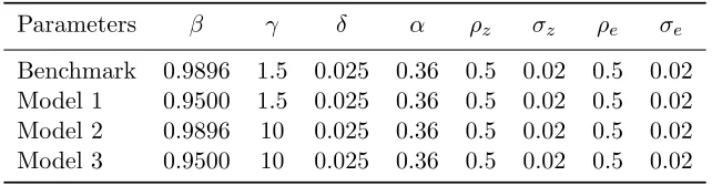
In order to reveal the power of the new algorithm, I also conduct some sensitivity analyses.
The sensitivity analyses focus on two parameters: the subjective discount factorβ and relative risk aversion coefficient γ. Model 1 changes β to 0.95 from the benchmark value; Model 2 changes γ to 10 from the benchmark value; Model 3 changes both.
Table 2.1: Parameters Calibration
Parameters β γ δ α ρz σz ρe σe
Benchmark 0.9896 1.5 0.025 0.36 0.5 0.02 0.5 0.02
Model 1 0.9500 1.5 0.025 0.36 0.5 0.02 0.5 0.02
Model 2 0.9896 10 0.025 0.36 0.5 0.02 0.5 0.02
Model 3 0.9500 10 0.025 0.36 0.5 0.02 0.5 0.02
2.5.2 Some Preliminary Results
First of all, I plot some selected policy functions in Figure 2.1. To make the explanation simple,
I plot only five policy functions where the aggregate capital is set toK = 40.70, the aggregate shock is set toz= 1,and the idiosyncratic shock takes five different values. The result is similar to Krusell and Smith (1998) in that the policy functions are almost linear across the whole
domain. Actually, only when the individual capital level is extremely low and the idiosyncratic
10
0 0.5 1 1.5 2 2.5 3 3.5 4 4.5 5
0 1 2 3 4 5
individual capital tomorrow
individual captial today Policy functions
et = e 1
et = e 2
et = e3
et = e 4
et = e5
Figure 2.1: Individual Policy Functions of the Benchmark Calibration
efficient labor shock is enormously bad (e=e1), will the policy function look a little nonlinear.
Since the policy functions are almost linear, and very few agents are binding, the property of
approximated aggregation holds. As explained by Krusell and Smith (2006), since the policy
functions are (almost) linear and very few agents are borrowing constrained, the marginal
propensity of saving is almost the same across agents. Therefore, the distribution of capital
does not matter, and one can simply use the first moment of the capital distribution to predict
the aggregate capital of the next period.
As mentioned earlier, the equilibrium of this model has to satisfy the consistency condition.
The consistency condition means that the law of motion of aggregate capital implied by the
model must mimic the overall outcome of heterogeneous agents. To check this, the procedure is
as follows. First, one needs to simulate a huge number of heterogeneous agents who face their
own idiosyncratic efficient labor shocks and the same aggregate shocks. Next, calculate the
aggregate capital through simulated data. Finally, one needs to compare the simulated capital
movement with the implied law of motion from the model.
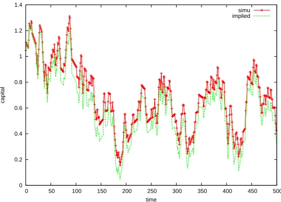
To do this simulation experiment, the number of heterogeneous agents is set to 10,000. The
0 0.2 0.4 0.6 0.8 1 1.2 1.4
0 50 100 150 200 250 300 350 400 450 500
capital
time
simu implied
Figure 2.2: Simulated Value of Aggregate Capital of Benchmark Calibration
that the initial state of the distribution does not determine or bias the implied aggregate law
of motion. The idiosyncratic shocks and aggregate shocks are simulated from the first order
Markov Chains, which reflects the setting of AR(1) processes. The simulation results are shown
in Figure 2.2. As can be seen, the implied aggregate law of motion nicely traces the movement
of the simulated aggregate law of motion that is solved from the model.
Other than looking at the evolution of aggregate capital, one can also check the so called
Euler equation residual to examine whether or not the solution is correct. The Euler equation
residual of this model is
residual=
ct−
n
minnV˜k(kt+1, et, Kt, zt),(1 +rt−δ)kt+wtet
oo−γ1
. ct
One can calculate the residuals on the domain of the state space,S. To calculate these residuals,
one needs to discretized the state space. For illustration purposes, I do not change the grid
numbers of aggregate capital or aggregate shocks; they are still set to 5. However, I increase
the number of grids for the individual capital to 1000, which are assumed to be equally-spaced.
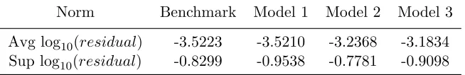
Table 2.2: The Euler Equation Residuals
Norm Benchmark Model 1 Model 2 Model 3
Avg log10(residual) -3.5223 -3.5210 -3.2368 -3.1834 Sup log10(residual) -0.8299 -0.9538 -0.7781 -0.9098
The interpretation of the Euler equation residuals is as follows. If log10(residual) =−4, it simply suggests that the agent will make a mistake of$1 when he consumes$10,000. As you can see from Table 2, the Euler equation residuals are pretty small if we examine the residuals from
the average norm. However, if we look at the residual from the sup norm, the performance is
somewhat unsatisfactory. This is merely a consequence from interpolation. When I calculate the
Euler equation residuals, I adopt the linear interpolation method. This interpolation approach
is, to some extent, flawed because the policy functions are somewhat nonlinear when individual
capital holding is close to zero and idiosyncratic efficient labor shocks are low. This problem
can be remedied by using nonlinear interpolation methods such as cubic splines.
2.5.3 Comparison with Existing Algorithms
The new algorithm I propose here is in many aspects better than some of the existing algorithms.
I briefly discuss the difference between the new algorithm, Krusell-Smith algorithm, and Xpa
in this subsection.
Comparing with Krusell-Smith (1998) The new algorithm is in essence utilizing the value function iteration, which is identical to Krusell and Smith (1998). However, in their algorithm,
Krusell-Smith employs a combination of the Newton method and the bisection method to find
the optimum of the right hand side of the Bellman equation. To implement the Newton method,
they resort to cubic splines for the dimension of individual capital. The bisection method is used
when the individual capital is lower than some level such that they can handle the problem of an
of zt, et, Kt in each value function iteration, one needs to do cubic spline interpolation once, making the computation very sluggish. Moreover, the adoption of bisection to handle a binding
constraint also creates problems. The reason is that one usually has no prior knowledge regarding
the bracket for the bisection method. This might not be a problem since a proper bracket can
be sometimes found by trial-and-error. However, it really becomes a problem if one would like
to conduct estimation, since the proper bracket varies with the combination of parameters.
The new algorithm does not need to resort to the Newton method and bisection. This
algorithm searches for the optimum of the right hand side of the Bellman equation through
the endogenous grid-point method of Carroll (2006). The backward solving structure of EGM
makes the search of the optimum of the Bellman equation trivial. Moreover, as explained in
step 2 in the last section, the EGM can naturally handle the binding constraint. Therefore, one
does not need to resort to the bisection method, and be troubled with the problem of finding
the proper bracket.
More importantly, the Krusell-Smith algorithm relies on simulation to update the aggregate
law of motion. To come up with the accurate aggregate capital, the number of individuals has to
be large; therefore, it usually takes a long time to update the aggregate law of motion. Moreover,
to ensure that the simulation is reliable, one needs to provide a good initial distribution for
the individual capital holding. If the initial distribution is not accurate enough, one needs to
discard a long series of simulation outcomes. This restriction might not be a serious problem if
the researchers only need to solve the model once. However, it becomes a serious problem when
implementing estimation tasks. In contrast, I follow the spirit of the explicit aggregation (Xpa)
method in the new algorithm. Therefore, the aggregate law of motion is obtained instantly
through the weighted average of individual policy functions, where the weights comes from the
exogenous ergodic distribution of idiosyncratic shocks. Since one can obtain the aggregate law of
motion from the policy functions during each iteration of the value function, one actually needs
to implement the value function iteration only once. It is a significant improvement compared
until the aggregate law of motion converges.
Comparing with den Haan and Rendahl (2010) The new algorithm is actually a mod-ification of the explicit aggregation from den Haan and Rendahl (2010). As I explained above,
this algorithm adopts explicit aggregation to update the aggregate law of motion. However, the
core of solving the models are different. In den Haan and Rendahl (2010), they use the Euler
equation based methods and, therefore, need to make assumptions on the shapes of the policy
functions in advance. If the original guess for the policy function is not quite good, the algorithm
can easily break down. Furthermore, it will become a problem when one needs to implement an
estimation task, since one usually does not have any prior knowledge about the policy functions
when the underlining parameters change. In contrast, the core of the new algorithm is the value
function iteration. The value function iteration method has nice convergence properties, which
have been proven mathematically. Theoretically, the value function will always converge since
the Bellman equation is a contraction mapping. In practice, all we need to do to implement the
new algorithm is to provide a monotonically increasing and concaved value function, which is
fairly straightforward. When one does so, the contraction mapping will automatically take care
of all other things. This is a significant advantage especially for the estimation task.
As mentioned earlier, having a fast and reliable algorithm is extremely important when one
estimates a heterogeneous agent model. I provide a comparison on the speed of the existing
algorithms in Table 2.3. There are some points that need to be mentioned regarding this table.
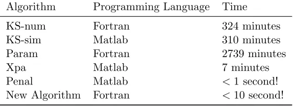
First, KS-num is the algorithm of Young (2010), and KS-sim is that of Maliar et al. (2010);
they are two different versions of the original Krusell-Smith (1998) algorithm. Param is the
algorithm proposed by Algan et al. (2008), and Penal is that of Kim et al. (2010). As you
can see, the Krusell-Smith type algorithms are very slow. The Param algorithm takes close to
two days to solve the model once. The Penal algorithm is extremely fast, but, as explained
above, this method does not solve the traditional heterogeneous agent model with borrowing
Table 2.3: Computation Time
Algorithm Programming Language Time
KS-num Fortran 324 minutes
KS-sim Matlab 310 minutes
Param Fortran 2739 minutes
Xpa Matlab 7 minutes
Penal Matlab <1 second!
New Algorithm Fortran <10 second!
*The model that implements the Penal algorithm is not
exactly the same as the others. Moreover, the model used here for comparison is that of den Haan et al. (2010), which is a slightly modification of Krusell and Smith (1998).
speed is acceptable for estimation task. Finally, the algorithm I provide in this chapter is
noticeably faster compared to all the existing algorithms.
2.6
Conclusion
This chapter proposes a new algorithm for solving computationally challenging heterogeneous
agent (HA) models. The algorithm combines the value function iteration (VFI) method, the
endogenous grid points method (EGM), and the explicit aggregation (XPA) method. This new
algorithm is robust in the sense that the initial values are irrelevant for finding the optimal policy
functions. Moreover, it is also fast because both the root-finding procedure for the household
problem and the repeated simulation for the aggregate law of motion are not necessary. The
algorithm solves a typical HA model within just a few seconds in a ordinary desktop computer.
As a consequence, it could be a proper tool for structural estimation of HA models, which needs
Chapter 3
Estimation of Heterogeneous Agent
Models
3.1
Introduction
It is well known that macroeconomic models have improved significantly in the modeling
strat-egy and explaining some stylized facts in the past two decades. The development of New
Keyne-sian (NK) models plays an indispensable role. In addition to having a better micro-foundation,
NK models incorporate several frictions and thus provide better descriptions of reality than
the traditional macroeconomic models. Besides, because of the advance in econometric
meth-ods, the implications of NK models can be explored by estimation rather than calibration. In
short, estimable NK models make them suitable for answering quantitative questions such as
the magnitudes of real effects due to a particular government policy.
The development of macroeconomics conveys two important messages. The first message is
about model setting. As explained by Sims (1996), models should be constructed to explain
observable real data. NK models incorporate the potential frictions in the real data. Therefore,
these models provides more explanatory power for puzzling macro phenomena. For example,
re-sponse with respect to monetary shocks. The second message is about the importance of model
estimation. Current macroeconomic models are complicated, because they often involve
dynam-ics of many endogenous variables and rational expectations of agents. Thus, the predictions of
models are sensitive to the change of parameter values. For example, the duration of real
out-put increases responding to a unexpected technology shock crucially depends on the persistence
coefficient of the technology shock. Thus, to obtain a better understanding of the underlying
structure of the economy, precise estimation of structural parameters is crucial.
While we have seen huge progress in the field of macroeconomics, up to now, all of the
estimated DSGE models resort to the representative agent paradigm. See An and Schorfheide
(2007), Smets and Wouters (2007), Christiano et al. (2005) for examples. However, the main
justification of a representative agent is that individuals are able to trade their risks in complete
markets. Unfortunately, complete markets are usually rejected in empirical studies. In other
words, the quantitative implications of these models might be imprecise or biased if the complete
markets assumption is far from reality.
To address this shortcoming, economists have already developed several heterogeneous agent
(HA) models. See for example, Aiyagari (1994), Huggett (1993), Krusell and Smith (1998), and
Quadrini (2000). The existing HA models have incorporated various sources of heterogeneity
such as health, age, marriage, unemployment, and preference. These improvements make HA
models a strong alternative to the traditional representative agent models. Unfortunately, an
important drawback still exists: None of these models is estimated by rigorous econometric
methods. In essence, the analysis of HA models still relies on calibration. As noted, calibrated
models are not suitable to answer quantitative questions unless accurate parameters are used.
According to An, Chang, and Kim (2009), the representative agent model often fails to
represent an equilibrium outcome of a heterogeneous agent economy. The fundamental reason
for this is that models are misspecified when one fails to take into account the presence of
heterogeneity in the real economy. A direct result of this is that parameter estimations are
estimate a model with heterogeneous agents.
Moreover, because of the adoption of the representative agent framework, economists usually
use only aggregate data for estimation, such as aggregate output and consumption. This implies
that some other useful information is actually left unemployed. For example, the U.S. Bureau
of Economic Analysis (BEA) provides a comprehensive household consumption data, known
as CEX. This dataset is widely used in analyzing household consumption related issues under
partial equilibrium, but rarely used for macroeconomic models under general equilibrium. With
HA models, micro-level consumption data can be conveniently utilized in estimation to help us
examine and better understand more aspects of the economy.
Thus, the motivation of the chapter is to address the mentioned shortcomings in modern
macroeconomic studies. Specifically, we estimate a heterogeneous agent model under general
equilibrium by incorporating both aggregate and distributional data. This task is rather
ambi-tious. First of all, HA models are notoriously difficult to solve computationally. Second, unlike
the representative agent models, in which the standard procedures for estimating them are
fairly established (see Canova (2007) and DeJong and Dave (2007)), the applicable literature
does not exist for the estimation of HA models under general equilibrium. Thus, there is a need
for us to provide our own procedure for it.
In regards to the first issue, we adopt the algorithm presented in the first chapter, which is
not only computational efficient but also robust in the sense that educated guesses for initial
values are not necessary. As for the second issue, we combine two simulation-based estimation
methods, i.e., Indirect Inference and Laplace-Type estimator, to formulate a hybrid estimation
method.
The structure of this chapter are as follows. We review the relevant literature in Section 3.2
and lay out an HA model in Section 3.3. The empirical methodology is discussed in Section 3.4.
Section 3.5 contains a short description of how data are being used. Lastly, Section 3.6 covers
3.2
Literature Review
3.2.1 Review of Heterogeneous Agent Models
Huggett (1993) constructs a heterogeneous agent model in which individual agents face
idiosyn-cratic income shocks. The only asset that individuals use to insure idiosynidiosyn-cratic shocks is the
riskless bond. 1 Moreover, he assumes that individuals cannot borrow without limit. That is, every individual faces a potentially binding borrowing constraint. Because of the possibility of
low income and the borrowing constraint, individuals exhibits precautionary saving behavior.
Under this formulation, Huggett (1993) provides an explanation for the cause of low real interest
rates, which has been viewed as a puzzle under the representative agent model.
Aiyagari (1994) considers a production economy with heterogeneous agents, and capital,
rather than a riskless bond, is used for insuring idiosyncratic shock. Similar to Huggett (1993),
he shows that the interest rate, aggregate capital, and wealth distribution can be coherently
determined through the precautionary saving motive, which stems from the borrowing
con-straint under the heterogeneous agent setting. His paper has now become an indispensable part
of modern heterogeneous agent models. However, the prediction about the wealth distribution
in the model of Aiyagari (1994) is not satisfactory. The Gini coefficient is too low and the rich
accumulate too little wealth, which conflict with what we observe in real data.
Quadrini (2000) extends the Aiyagari model to accommodate occupational choice. By
includ-ing endogenous occupational choice, his model fits surprisinclud-ingly well with the wealth distribution
and socioeconomic mobility of the United States. In his calibrated model, the top 1 percent of
rich households holds 24.9 percent of total wealth and the empirical counterpart is 26 percent
in the Panel Study of Income Dynamics (PSID) data.
The model of Krusell and Smith (1998) is the first heterogeneous agents model that
incorpo-rates aggregate uncertainty. They provide an algorithm based on a property calledapproximate aggregation. Krusell et al. (2009) use a calibrated model to investigate the welfare effect of
1
removing business cycles, which is a famous issue in economics introduced by Lucas (1987).
2 However, Krusell et al. (2009) find that the welfare gain under their heterogeneous agents
model is an order of magnitude larger than that of Lucas. Moreover, their calibrated model
shows that there are large differences across groups: Very poor consumers gain a lot, and so do
very rich consumers. However, the majority of consumers (middle class) gain little. That is, the
improvement of welfare is U-shaped across wealth levels.
The heterogeneous agent models are growing fast now and most of the early literature
focused on the heterogeneity of income or wealth. However, heterogeneity of the economy is not
limited in this sole dimension. For instance, Palumbo (1999) shows that health status is a key
driving process for the saving decision of the elderly, and Cubeddu and Rios-Rull (2003) finds
that marital status risk is a larger source of precautionary saving than income risk.
3.2.2 Review of Empirical Studies
Gourinchas and Parker (2002) construct a dynamic stochastic model to analyze the life cycle
saving behavior of heterogeneous agents. Each agent faces an exogenous, stochastic labor income
process. The income process of each agent is a function of agent’s characteristics, including
education level, occupational type, and age. Moreover, to make the model more flexible, they
allow the utility function to be a function of agents’ characteristics. That is, the heterogeneity
of the economy stems not only from the difference in income level or wealth but also from the
diversity in agents’ preferences.
They construct average consumption and income profiles across the households of five
differ-ent educational levels and four occupational groups. The data they use to construct
consump-tion and income profiles are the Consumer Expenditure Survey (CEX), which contains roughly
40,000 households from 1980 to 1993. After constructing the consumption and income profiles,
they numerically solve the life-cycle model and generate a theoretical consumption profile. By
comparing the theoretical consumption profile to that of the empirical one, they estimate the
2Lucas uses a representative agent model to quantify the welfare effect of removing the business cycle, and