* Corresponding author. Fax: +98-21-88465131 E-mail: [email protected] (A. Aghaie) © 2011 Growing Science Ltd. All rights reserved. doi: 10.5267/j.ijiec.2011.01.007
Contents lists available at GrowingScience
International Journal of Industrial Engineering Computations
homepage: www.GrowingScience.com/ijiecHat and squeeze functions, a way for making precise algorithms
Elham Shadkama and Abdollah Aghaiea*
aDepartment of Industrial Engineering, K.N. Toosi University of Technology, Vanak, Tehran, Iran
A R T I C L E I N F O A B S T R A C T
Article history:
Received 4 November 2010 Received in revised form 22 January 2011
Accepted 22 January 2011 Available online 27 January 2011
Random variates play key role in any simulation system and there are different algorithms to generate random variates. One of the best algorithms for generating random variates is uniform fractional part algorithm. The algorithm has high performance in terms of efficiency, speed and simplicity. Although the algorithm has useful results, it is an approximate algorithm. In this article, the approximate form of the algorithm has been studied, and some suggestions have also been presented. Through acceptance-rejection approach and hat and squeeze function, the approximate algorithm is transformed to near exact algorithm. The proposed model of this paper has been examined and compared with the traditional one and the preliminary results indicate that it performs better than the other existing algorithms.
© 2011 Growing Science Ltd. All rights reserved
Keywords:
Random Variate Generation Hat and Squeeze Functions Uniform Fractional Part Algorithm
Approximate State
1. Introduction
Random variates play an important role on the implementations of simulation techniques. During the past few years, there has been an increasing interest in development of new techniques based on random variates. In this article, we introduce a new method to generate random variates from continuous distributions. The proposed algorithm called uniform fractional part (UFP) seems to be simpler and more efficient compared with other methods of random variates generation despite the fact that the method is an approximate one. The primary goal of this article is to present a new near exact algorithm based on the previously published work of Ahrens and Dieter (1982).
The combination method is used when distribution function (F) is presentable as convex combination of other distributions of F , F , etc shown in Eq. (1). This method is applicable to discrete and continuous distributions.
(1)
F x P F x
∞
.
Convolution method is used for distributions in which the value of X can be shown as a sum of random variates which is easier than a direct generation of X. In other words, we assume that y , y ،...،y exist such that the sum of these values have the same distribution as of X.
When other methods are not applicable, acceptance-rejection method is used. In this method, a hat function is considered for the main function in such a way that the generation of variates is easier than this hat function. The proposed model of this paper is based on acceptance-rejection method and the details of the implementation is presented in this paper.
2. Classifications of generation algorithms of random variates
In order to have a better understanding of characteristics of different methods for generating random variates a summary of all these methods are presented in Table 1.
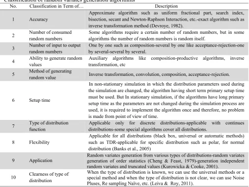
Table 1
Classification of random variates generation algorithms
Description Classification in Term of…
No.
Approximate algorithm such as uniform fractional part, search index, bisection, secant and Newton-Raphson Interaction, etc.-exact algorithm such as inverse transformation method (Devroye, 1982).
Accuracy 1
Some algorithms require a certain number of random numbers, but in some algorithms the number of random numbers is random itself.
Number of consumed random numbers 2
One by one such as composition-several by one like acceptance-rejection-one by several-several by several.
Number of input to output random numbers
3
Auxiliary algorithms like composition-productive algorithms, inverse transformation, etc
Ability to generate random values
4
Inverse transformation, convolution, composition, acceptance-rejection. Method of generating
random value 5
In non-stationary simulation in which the distribution parameters used during the simulation are changed, the algorithm having short term primary setup time must be used. But In stationary simulation, if the algorithms have long primary setup time as the parameters are not changed during the simulation process are used, it is required to implement the algorithm once and therefore, no problem is made from point of view of time.
Setup time 6
Applicable only for discrete distributions-applicable with continues distributions-some special algorithms cover all distributions.
Type of distribution function
7
Applicable for all distributions (black box, universal or automatic methods) such as TDR-applicable for specific distribution such as polar, for normal distribution (Banks et al., 2005)
Flexibility 8
Random variates generation from various types of distributions-random variates generation of order statistics (Cheng & Feast, 1979)-generation independent random variates and truncated values (Kurowicka & Cooke, 2001).
Application 9
When the type of distribution is known, we can use the universal methods or a special method and when the type of distribution is not clear, we can use Noise Pluses, Re sampling Naïve, etc. (Leiva & Roy, 2011).
Clearness of type of distribution
10
independency from a machine, etc. (Hung et al., 2010). The method under the study of this article, uniform fractional part algorithm, almost covers all the mentioned criteria. Before we introduce uniform fractional part method, it is necessary to note that this method is one of the universal or black box methods. Although the algorithm has numerous advantages, it is an approximate algorithm. The object of this article is to improve precision of the existing algorithm. Initially, we introduce uniform fractional part or UFP, which is simpler and efficient compared with other methods of generating random variates. This method is based on a statistical hypothesis. First, the method and its applications are introduced, and then its near exact algorithm is presented.
3. Description of the uniform fractional part algorithm
This algorithm is one of the latest methods presented by Izady and Mahlooji (2005), and it is an approximate algorithm to be used for continues distributions. The algorithm is based on a theorem explained as an example on Morgan's book (1984, page 72). Since we need the details of the algorithm we explain the theorem in this section.
Theorem: fractional part of total two independent random variables with uniform distribution on
0,1 , itself has uniform distribution on 0,1 .
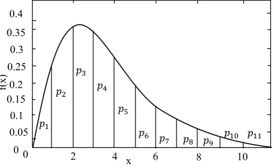
Fig. 1. Probabilities associated with x
The basic logic of the algorithm is as follows: Initially, an integer value in the scope of x is randomly selected (one column in Fig. 1) and then a value R R , where R and R are two independent uniform [0,1] random variables are added to make a random variate (Mahlooji et al., 2008).
Fig. 2. The performance of UFP method
versus the other methods in terms of time
Fig. 3. The performance of UFP method versus
the other methods in terms of p-value
Fig. 2 and Fig. 3 show the advantage of UFP algorithm in terms of the speed and the precession compared with other techniques for generating random variates using Gamma distribution. To measure how well the data follow a particular distribution Kolmogorov-Smirnov statistic is used. Obviously, the better the distribution fits the data, the smaller this statistic will be. The lower this statistic is, the bigger test p-values will be which means a better precision of the algorithm. Although
0 0.4 0.35
0.3
0.25 0.2
0.15 0.1 0.05
4
6
2
0 8 10
f(x)
some algorithms are more accurate than UFP, their accuracy changes with the modification of the parameters and they are not considered robust but UFP is robust with respect the distribution parameters.
There are 9 algorithms considered for generating random variates. The random variates generated by algorithm 1, 2 and 3 follow continues distribution function with cut off point, arbitrary cut off points and equal area approach, respectively. Algorithm 4 is also based on continues distribution and uses different approaches to determine the tails of the distribution. Algorithm 5 applies continues distribution function with reduction approach for the number of random numbers used when d=1 and algorithm 6 repeats the same procedure using an arbitrary value, d. Algorithm 7 generates the random variates using continues distribution function with recycling uniform random number with d=1 and algorithm 8 uses an arbitrary d. Finally, algorithm 9 generates the random variates using continues distribution function based on generating int(x). The proposed model of this paper uses the idea of algorithm 9. Therefore, from the algorithms presented in UFP algorithm evolution, only the steps associated with the algorithm 9 is presented as follows:
1) Input p, uniform probability cut off points a , a , … , a and d a a for i 1, . . . , k 1,
2) generate the random number u′ (uniform [0,1] random variables),
3) calculate the value ′ 1 and determine the index i, then identify a value for int (x) based on the value of i,
4) generate the random number u on 0, d where d denotes the length of the interval into which X falls (uniform [0, d] random variables),
5) deliver X, as x ud a
4. UFP algorithms
Algorithm 1 is the primary algorithm of UFP in which the cut off points should have integer values. We also need to choose appropriate distribution parameters to maintain the independency condition. In the event where x does not follow uniform distribution there may be a correlation between R1 and
R2. Therefore, algorithm 2 removes the constraint associated with the determination of parameters
and cut off points include non-integer values. To determine cut off points of the algorithm, we can use two approaches of an equal area and variance increase. There are some studies which indicate that equal area approach has more advantages than the other ones (Mahlooji et al., 2008). One of the problems with UFP algorithm is its inefficiency for the distributions with unlimited boundary. Therefore, the solution presented by this algorithm needs to truncate the distribution tails and the algorithm 4 performs the foresaid work with the pre-determined precision.
5. Various applications of UFP algorithm
1. Generation of continues random variates such as Gamma, Beta, Normal, etc.: UFP algorithm can be used for various continues distribution such as Normal, Gamma, Beta, etc. and shows desired results in terms of speed and precision. According to Mahlooji and Izady (2004), the speed and precision of this method is robust against the changes of parameters.
2. Generation of correlated random variates: in some of the simulated models, there is a need to generate one random vector as X x , … , x T from one special joint distribution (or multi-variates) in which the single components of its vector may not be independent (Sak et al., 2010). UFP method is also usable in generation of such independent values in which for generation of two values with desired integrated marginal distributions having desired correlations, this issue causes no need of making joint function (Mahlooji & Izady, 2004).
3. Generation of random variates associated with ordering statistics: UFP method is also usable for order statistics. Since this method does not need index search as a part of the algorithm, it is faster than the other methods for order statistics (Mahlooji et al., 2004).
4. Generation of random numbers: UFP algorithm has the capability of fast generation of random numbers in which UFP and alias have been combined and the final algorithm is named UFPG (Mahlooji et al., 2004). Despite linear congruential generators and multiplicative recursive generators which have limited length, the length of this generator is almost unlimited (its course length is more than four billions) and has various advantages such as transfer capability, repeatability, short term primary setup time and passing the various statistical tests (such as run, discrepancy and correlation).
6. The basics of Acceptance-rejection technique
Von Neumann (Banks, 1998) presented the main idea of this method. In acceptance-rejection method, in order to generate random points in some of the hard and complicated areas A, it is enough to find a simpler area such as B in such a way that the area A is covered.Then starting from region B, random points are generated and if the points are also located in the area A, they will be introduced as accepted points. Therefore, the accepted points will be distributed uniformly in the interval A and the method is called acceptance-rejection method
.
Squeeze method is a skilled one to promote the efficiency of acceptance-rejection methods. In this method, it is supposed that C is an area to be surrounded by A and also D is another area to surround A in such a way that D A C. Squeeze function is used for evaluation of P points generated in B, which may or may not be located in A. To avoid time wasting, prior to evaluation of p A , if p D or p C, if P is located in D it is also located in A and if there is not P in C, P is not in A either. Efficiency of acceptance and rejection methods depends on two things: easiness and generation of variates from B and another one is the average number of variates generated from B for generation of a number of A (this quantity is defined as |A|Start
yes
No Generate u
If
Generate y
x=
this method to the mentioned method, we can use hat and squeeze functions with uniform density (Franklin & Sen, 1975). The following assumptions hold with acceptance and rejection method.
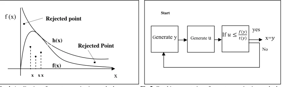
1. another function exists such as h(x) to surround f(x) (it means h x f x for all Xs in Fig. 4)
2. It is possible to generate the random variate from distribution h(x), such points are shown by x, y .
3. If the graph f(x) is drawn, in this case, the point (x,y) is located in above or below of f(x) curve (y x or y f x ).
The most important factor to determine the desired value is to minimize the space between the two charts h and f based on minimizing the number of rejected points. The next important factor in determining h is to speed up the generation of variates from this distribution. The average number of required points (x,y) to generate an accepted x is to find the trial rate. It is obvious that the number of trial rate in an ideal state is equal to one (Ormann & Erflinger, 1994). The logic of acceptance-rejection method is shown in Fig. 5.
Fig. 4. Application of acceptance-rejection method Fig 5. Graphic presentation of acceptance-rejection method
7. The use of acceptance-rejection method on UFP algorithm
Since the main method (algorithm 9 that is named A′ method) is an approximate one, by defining a
hat function h(x) and through the use of acceptance-rejection logic, it can be transformed to a near exact method. Hat function defined for x, located in the interval a , a is uniformly defined on
0, f a . The logic for using hat function is that if for the random pair x, y (in which x is
generated from any method and y is generated from a hat function), the inequality y f x is satisfied then the generated points are dispersed uniformly under f(x) density function and consequently, the points have f(x) distribution (because y values are under the density function f x and has it has a uniform distribution). Nevertheless, in algorithm A, evaluation of acceptance condition is a time consuming step for most of distributions. Therefore, the speed of algorithm may increase when squeeze function is used. Therefore, a lower limit of S(x) should be found in such a way that inequality s x f x holds. In this case, if x, vh x (v is uniform [0,1] random variables and h(x) is hat function) pair values is under S(x) (Squeeze function), we can accept random variate x without evaluation of density function. In fact, in algorithm A, local or piecewise hat function and in B, local or piecewise squeeze function are used. Determination of hat and squeeze function depends on the form of the function. If the function is descending (such as Fig. 6), hat function for each 0, f a interval is determined and squeeze function is considered uniformly on 0, f a interval. If the foresaid function is an ascending one (fig 7), the hat function is uniform on 0, f a interval and squeeze function is considered uniformly on 0, f a interval. We apply the definitions of squeeze and hat functions in descending situation due to frequency in different distribution functions, although the other definitions of hat and squeeze functions are also applicable to UFP algorithm.
x x
Rejected Point
f(x)
Rejected point
h(x)
x f (x)
Algorithm A (UFP algorithm with hat function) Algorithm B (UFP algorithm with hat and squeeze function) 1) generate x with ′ algorithm,
2) generate a random number ~ 0,1 , 3) calculate the value of , 4) if , then, return x (evaluated
step for PDF), otherwise; go to step 1.
1) generate x with ′ algorithm,
2) generate a random number ~ 0,1 , 3) calculate the value of ,
4) if , then, return x (evaluated step for squeeze function), otherwise; go to step 5. 5) If , then, return x (evaluated step for PDF),
otherwise; go to step 1.
Fig. 6. Hat and squeeze function for descending functions Fig. 7. Hat and squeeze function for ascending functions
Now a situation is considered that the function has maximum and minimum points (fig. 8 and Fig. 9). If the foresaid interval includes (M) modes or minimizing points, in this case, the hat function is uniformly defined on 0, f M interval and squeeze is as uniform on 0, f a interval.
Fig. 8. Hat and squeeze function for the function has minimum point Fig. 9. Hat and squeeze function for the function has maximum point
If the interval is located before or after maximizing or minimizing point, the hat and Squeeze function is considered as determined, previously. If the foresaid distribution functions have a more complicated form, we define hi and si as follows,
(2)
: ,
(3)
: .
Therefore, hat and squeeze functions are generated uniformly on 0, h and 0, s . Since we ignore many conditions to determine si and hi, the performance of the proposed method will be increased.
8. Verification of the presented approach
For verification of the presented corrective approach, the improved algorithms obtained from this approaches are compared with the original one. Exponential distribution has been used for comparison. Of course, the improved algorithm is applicable for all other continuous distributions. As mentioned, the proposed algorithm is the universal one and has no limitation of use for any special distribution.
ai ai+1 f(x) h(x)= f(ai+1)
s(x)= f(ai)
f(x) h(x)= f(ai)
s(x)= f(ai+1)
ai ai+1 an
f (x)
x
f (x)
For validation, two criteria of speed and precision are used. For speed criterion, one million random data have been generated and generation speed has been calculated based on random variate µs. For precise criterion also, we calculated P-value parameter based on Anderson-Darling test with 95% confidence level. It is worth to mention that the tests have been performed with Borland compiler of C++ 5.02 under 32-Bit platform and evaluation parameters have been calculated using Minitab software. Anderson-Darling's A2 statistic defined as follows:
(4)
A n 1
n 2i 1 ln F x ln 1 F x
The assumption under the study in this test is as follows: H0: The data follow a specified distribution
H1: The data do not follow a specified distribution
It is worth to mention that presented times in the tables are only for comparison between the original method and the improved one. More professional coding can reduce the amount of generating time, greatly. An example of generation time of random variates for Beta distribution with other methods presented in Table 2 with a more advanced coding program. Because our objective is the comparison, the coding has been simplified in this article (Izady, 2005).
Table 2
comparison with UFP method with other methods from speed point of views
Algorithm UFP TDR BPRB BPRS B4PE Sakasegawa Cheng Strip NI Johnk
Speed(µs) 0.25 1.3 2.3 1.85 2.1 2.7 3.3 1.5 1.4 6.62
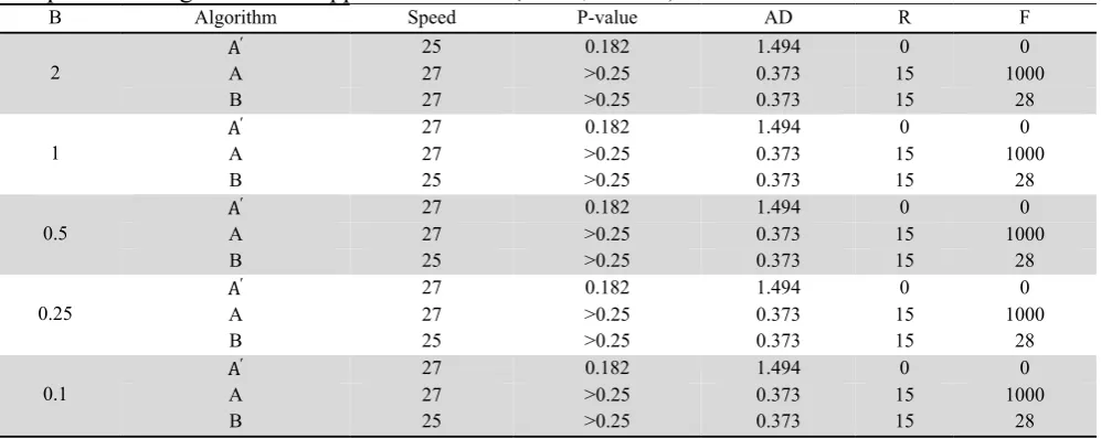
Table 3
Comparison of algorithms for approximate state (N=128, P=1/128)
Table 3 shows the result of comparison of various criteria for three algorithms based on exponential distribution with various parameters. In the following table, AD means Anderson-Darling test statistic value, and R is the numbering average of values rejected from 1000 generated random values. f means the number of density function evaluation for generation of 1000 random variates. Number of cut off points in Table 3 is equal to 128 sections, which are considered as power of two, and it is due to capability of programming language for powers of two. As we can observe from Table 3, the foresaid methods are robust and stable compared with the changes of distribution parameters. In terms of precision, Algorithm A provides higher P-values and lower Anderson-Darling statistic value than ′. Therefore A is more precise than A'. In addition, algorithm B seems to be faster compared
with two other algorithms. It is due to decreasing number of density function evaluation, which is
F R
AD P-value
Speed Algorithm
B
0 0
1.494 0.182
25
A′
2 A 27 >0.25 0.373 15 1000
28 15
0.373 >0.25
27 B
0 0
1.494 0.182
27
A′
1 A 27 >0.25 0.373 15 1000
28 15
0.373 >0.25
25 B
0 0
1.494 0.182
27
A′
0.5 A 27 >0.25 0.373 15 1000
28 15
0.373 >0.25
25 B
0 0
1.494 0.182
27
A′
0.25 A 27 >0.25 0.373 15 1000
28 15
0.373 >0.25
25 B
0 0
1.494 0.182
27
A′
0.1 A 27 >0.25 0.373 15 1000
28 15
0.373 >0.25
time consuming. In method A, for generation of 1000 random variates, we need 1000 times of density function evaluation. This value was decreased to 28 times for algorithm B, which causes speeding up the algorithm. The results show that by increasing the value of statistics, the number of density function evaluation and also the number of failed values of the algorithm shall decrease the precision of the algorithm. Therefore, as far as the value of these two parameters is low, it shows the good performance of the proposed algorithm. Afterwards the impact of the number of cut off points changes on other factors such as P-value of test, Anderson-Darling statistic value, the number of failed value and the number of density function evaluation shall be studied (Table 4-8).
Table 4
The impact of the number of cut off points on speed of the algorithm
P=1/64 P=1/128 P=0.0025 P=0.005 P=0.01 p=0.02 p=0.05 Algorithm
Β N=20 N=50 N=100 N=200 N=400 N=128 N=64
S S S S S S S 27 27 32 31 31 31 31 A′
2 A 31 31 31 31 32 27 27
25 25 28 28 28 28 28 B 27 27 32 31 31 31 31 A′
1 A 31 31 31 31 32 27 27
25 25 28 28 28 28 28 B 27 27 32 31 31 31 31 A′
0.5 A 31 31 31 31 32 27 27
25 25 28 28 28 28 28 B 27 27 32 31 31 31 31 A′
0.25 A 31 31 31 31 32 27 27
25 25 28 28 28 28 28 B 27 27 32 31 31 31 31 A′
0.1 A 31 31 31 31 32 27 27
25 25 28 28 28 28 28 B Table 5
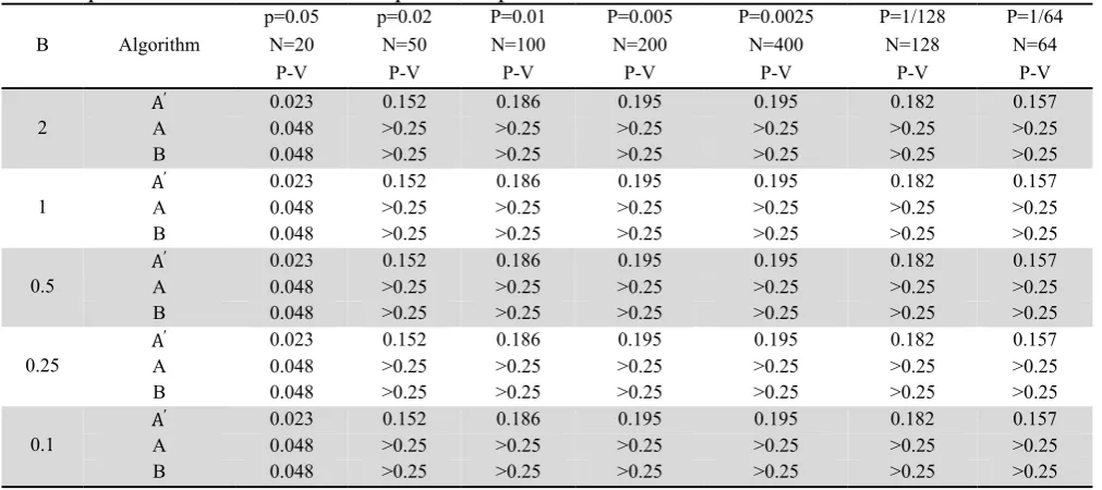
The impact of the number of cut off points on p-value of test
P=1/64 P=1/128 P=0.0025 P=0.005 P=0.01 p=0.02 p=0.05 Algorithm
Β N=20 N=50 N=100 N=200 N=400 N=128 N=64
P-V P-V P-V P-V P-V P-V P-V 0.157 0.182 0.195 0.195 0.186 0.152 0.023 A′
2 A 0.048 >0.25 >0.25 >0.25 >0.25 >0.25 >0.25
>0.25 >0.25 >0.25 >0.25 >0.25 >0.25 0.048 B 0.157 0.182 0.195 0.195 0.186 0.152 0.023 A′
1 A 0.048 >0.25 >0.25 >0.25 >0.25 >0.25 >0.25
>0.25 >0.25 >0.25 >0.25 >0.25 >0.25 0.048 B 0.157 0.182 0.195 0.195 0.186 0.152 0.023 A′
0.5 A 0.048 >0.25 >0.25 >0.25 >0.25 >0.25 >0.25
>0.25 >0.25 >0.25 >0.25 >0.25 >0.25 0.048 B 0.157 0.182 0.195 0.195 0.186 0.152 0.023 A′
0.25 A 0.048 >0.25 >0.25 >0.25 >0.25 >0.25 >0.25
>0.25 >0.25 >0.25 >0.25 >0.25 >0.25 0.048 B 0.157 0.182 0.195 0.195 0.186 0.152 0.023 A′
0.1 A 0.048 >0.25 >0.25 >0.25 >0.25 >0.25 >0.25
Increasing the number of division causes the shortening of p and consequently, increasing the algorithm precision. Therefore, if p goes toward zero, the precision of this algorithm approaches the precision of other exact methods such as inverse transformation method. As it is observed all criteria under study shall be remained robust by changing exponential distribution parameter.
Table 6
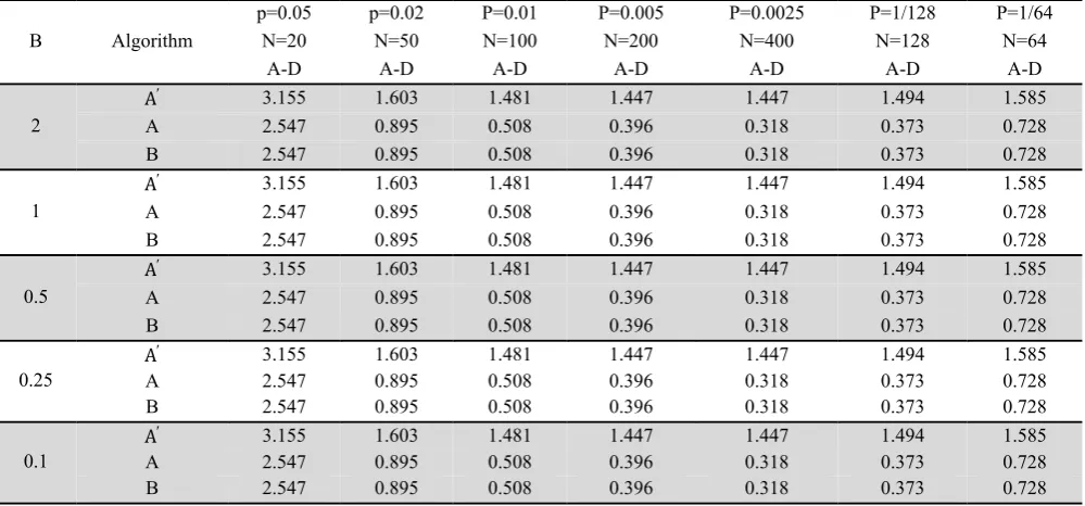
The impact of the number of cut off points on Anderson-Darling statistic value
P=1/64 P=1/128 P=0.0025 P=0.005 P=0.01 p=0.02 p=0.05 Algorithm
Β N=20 N=50 N=100 N=200 N=400 N=128 N=64
A-D A-D A-D A-D A-D A-D A-D 1.585 1.494 1.447 1.447 1.481 1.603 3.155 A′
2 A 2.547 0.895 0.508 0.396 0.318 0.373 0.728
0.728 0.373 0.318 0.396 0.508 0.895 2.547 B 1.585 1.494 1.447 1.447 1.481 1.603 3.155 A′
1 A 2.547 0.895 0.508 0.396 0.318 0.373 0.728
0.728 0.373 0.318 0.396 0.508 0.895 2.547 B 1.585 1.494 1.447 1.447 1.481 1.603 3.155 A′
0.5 A 2.547 0.895 0.508 0.396 0.318 0.373 0.728
0.728 0.373 0.318 0.396 0.508 0.895 2.547 B 1.585 1.494 1.447 1.447 1.481 1.603 3.155 A′
0.25 A 2.547 0.895 0.508 0.396 0.318 0.373 0.728
0.728 0.373 0.318 0.396 0.508 0.895 2.547 B 1.585 1.494 1.447 1.447 1.481 1.603 3.155 A′
0.1 A 2.547 0.895 0.508 0.396 0.318 0.373 0.728
0.728 0.373 0.318 0.396 0.508 0.895 2.547 B Table 7
The impact of the number of cut off points on number of failed value
P=1/64 P=1/128 P=0.0025 P=0.005 P=0.01 p=0.02 p=0.05 Algorithm
Β N=20 N=50 N=100 N=200 N=400 N=128 N=64
R R R R R R R 0 0 0 0 0 0 0 A′
2 A 66 35 18 10 8 15 29
29 15 8 10 18 35 66 B 0 0 0 0 0 0 0 A′
1 A 66 35 18 10 8 15 29
29 15 8 10 18 35 66 B 0 0 0 0 0 0 0 A′
0.5 A 66 35 18 10 8 15 29
29 15 8 10 18 35 66 B 0 0 0 0 0 0 0 A′
0.25 A 66 35 18 10 8 15 29
29 15 8 10 18 35 66 B 0 0 0 0 0 0 0 A′
0.1 A 66 35 18 10 8 15 29
29 15 8 10 18 35 66 B
9. The performance of the algorithm B based on theoretical and experimental results
of the distribution and divide the region of the exponential distribution into 128 segments with
β 0.25 and s x f a and h x f a . Therefore we have,
A 1.0117689496751, A 0.973862463238 and A 0.999. Since we have,
(5)
α A
A ,
A A
Table 8
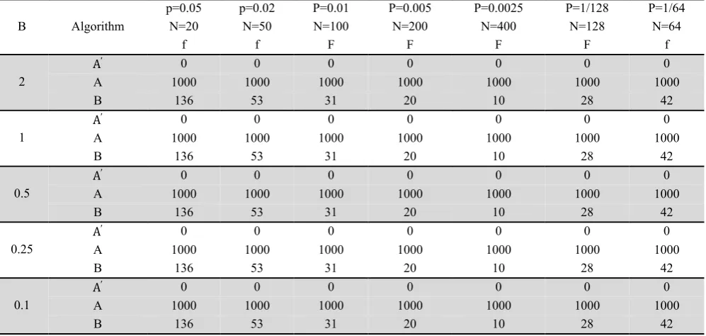
The impact of the number of cut off points on the number of objective function evaluation times
P=1/64 P=1/128 P=0.0025 P=0.005 P=0.01 p=0.02 p=0.05 Algorithm
Β N=20 N=50 N=100 N=200 N=400 N=128 N=64
f F F F F f f 0 0 0 0 0 0 0 A′
2 A 1000 1000 1000 1000 1000 1000 1000
42 28 10 20 31 53 136 B 0 0 0 0 0 0 0 A′
1 A 1000 1000 1000 1000 1000 1000 1000
42 28 10 20 31 53 136 B 0 0 0 0 0 0 0 A′
0.5 A 1000 1000 1000 1000 1000 1000 1000
42 28 10 20 31 53 136 B 0 0 0 0 0 0 0 A′
0.25 A 1000 1000 1000 1000 1000 1000 1000
42 28 10 20 31 53 136 B 0 0 0 0 0 0 0 A′
0.1 A 1000 1000 1000 1000 1000 1000 1000
42 28 10 20 31 53 136 B
The probability of specified number of iterations for generating one random variate is p I i
α 1 α . The expected number of iterations also is E I α . The variance of the number
of iterations is var I α α 1 and the expected number of evaluations of f (density function) for generating one random variate is E #f AA 1. The area between hat and squeeze also
is A A A 0.03790648 and
α 1.012781731, 1.03892386, p I 1 0.9873795 , p I 2 0.0124.
As we can see, normally, we only need single repetition of the algorithm to generate a random value with a given probability, say 99%. The other observation is that we only need a few number iterations to reach the final solution. For instance, in this case, we needed only two iterations to reach the desired accuracy of 0.012%. For this example, the final solution had a small variance of 0.0129 which is a significant small value. Our experimental results also indicate that we need only a few density function evaluation. In order to verify our results, we calculate AH and ASboth theoretically and experimentally using the following,
AH i d f a , AH ∑ AH i AS i d f a , AS ∑ AS i , A 1 0.001 0.999. In experimental state 1000 data have been generated and the foresaid conditions in table 9 are met.
Table 9
Therefore, the obtained results are as follows: E #f 0.028,α E I 1.015228 . It is interesting to see that the empirical results confirm the theoretical findings.
10. Conclusions
In this work, we introduced the importance of random variates in simulation and presented an explanation and classification about different random variates algorithms. The proposed model of this paper also presented a transformation approximate algorithm as a near exact UFP method. Our findings indicate that near exact UFP method outperforms approximate UFP method in generating random variates. Future research may be about making all relations theoretical, which has been performed in the article as experimental and simulation.
References
Ahrens, J. H., & Dieter, U. (1982). Generating gamma variates by a modified rejection technique.
Communications of the ACM, 25, 47-54.
Banks, J., Carson, J. S., Nelson, B. L., & Nicol, D.M. (2005). Discrete-event system simulation. Upper Saddle River: Pear-son Prentice Hall.
Banks, J. (1998). Handbook of simulation principle, methodology, advances, applications, and practice. New York: John Wiley & Sons.
Cheng, R.C.H., & Feast, G.M. (1979). Some simple gamma variate generators. appl statist, 28(3), 290-295.
Devroye, L. (1982). A note on approximations in random variate generation. Journal of Statistical Computation and Simulation, 14(2), 149-158.
Franklin, M.A., & Sen, A. (1975). Comparison of exact and approximate variate generation methods for the erlang distribution. Journal of Statistical Computation and Simulation, 4(1), 1-18.
Hormann, W., Leydold, J., & Derflinger, G. (2004). Automatic nonuniform random variate generation. New York: Speringer-Verlag.
Hung, Y. C., Balakrishnan, N., & Cheng, C.W. (2010). Evaluation of algorithms for generating Dirichlet random vectors. Journal of Statistical Computation and Simulation.
Kurowicka, D., & Cooke, R.M. (2001). Proce. the European Safety and Reliability Conference.
Torino, Italy: ESREL, 1795- 1802.
Leiva, R., & Roy, A. (2011). A Quadratic Classification Rule with Equicorrelated Training Vectors for Non Random Samples. Communications in Statistics-Theory and Methods, 40(2), 213- 231.
Mahlooji, H., Jahromi, A.E., Mehrizi, H.A., & Izady, N. (2008). Uniform Fractional Part: A simple fast method for generating continuous random variates. Scientia Iranica,15(5), 613-622.
Mahlooji, H., Mehrizi, H. A., & Farzan, A. (2004). A fast method for generating continuous order statics based on uniform fractional part. Proc. 35th International Conference on Computers and Industrial Engineering, 1355-1360.
Mahlooji, H., Mehrizi, H., & Sedghi, N. (2004). An efficient, fast and portable random number generator. Proc. 35th International Conference on Computers and Industrial Engineering, 1361-1366.
Mahlooji, H., & Izady, N. (2004). Developing a wide class of bivariate copulas for modeling correlated input variables in stochastic simulation. Proc.35th International Conference on Computers and Industrial Engineering, 1349-1354.
Mahlooji, H., & Izady, N. (2004). A new method for generating gamma values. Proc. International Conference on Industrial Engineering, 294-305.
Meuwissen, A. H. M., & Bedford, T. J. (1997). Minimal informative distributions with given rank correlation for use in uncertainty analysis. Journal of Statistical Computation and Simulation, 57, 143-157.
Morgan, B. J. T. (1984). Elements of simulation. London: Chapman and Hall.
Ormann, W., & Erflinger, G. (1994). The transformed rejection method for generating random variables, an alternative to the ratio of uniforms method. Communications in Statistics - Simulation and Computation, 23(3), 847 – 860.