C o n v e r g e n c e D e t e r m i n i n g C l a s s e s
i n t h e
C e n t r a l L i m i t T h e o r e m .
bv
J u l i a n C h a r l e s H . W i g h t w i c k .
A thesis submitted for the degree of Doctor of Philosophy at the Australian National University.
March 1986
D e c l a r a t i o n .
E x ce pt where ot her wi s e i ndi cat ed thi s thesis is my own work.
3
A c k n o w l e d g e m e n t .
1 would like to thank my supervisor. Peter Hall, for his persistent direction and encouragement.
4
A b s t r a c t .
Let X , X \, A'2, . . . be i n de pe nde nt , identically d i s t r i b u t e d r a n d o m variables wi t h zero m ea n and unit variance, and let Pn ( x) be t he d i s t r i b u t i o n function of n - 1 / 2 i X 3. T h e Cent ral Li mit T h e o r e m is often pres ent ed as a uni form bound on t he difference \Pn (x) - 4>(x)j as n —* oc, where <L(x) is t he S t a n d a r d Nor ma l d i s t r i b u ti o n function. Such an a pp r o a c h ignores a lot of i n f or ma t ion a b o u t t h e r a t e of convergence of P n (x) t o <L(x) at p a r t i c u l a r poi nt s x. Remar ka bl y, much of t hi s detailed i nf or mat ion does not d e p en d on t h e d i s t r i b u t i o n of X .
Given a set X of Real n um b e r s , p u t A n ( T ) = s u p xeX \Pn (x) - 4>(x)j. Hall (1982) defines a set X t o be convergence d e t er m i ni n g ( CD) if
lim inf 77 —♦ OC
A n ( X ) + n - P 2 \
A n ( R )
J
> 0for every choice of t h e d i s t r i but i on of A’; t h a t is. t he worst r a te of convergence of P n (x) to ^ ( x ) over x £ X is essentially no b e t t e r t h a n t he worst r a te over t h e whole Real line. Th e r e is a useful expansion due t o Osipov (1971) and Rozovskii (197-4):
s up Pn (x) - 4>(x) - Q n (x)i = o ( s up Q n {x) ) - 0 ( t i 1 2).
X R T o ) ■'
Hence t he "leading t er m Q n (x). which d e p e n d s on t h e d i s t r i b u ti o n of A . carries all t he i nf or mat ion needed to decide w h e t h e r or not a set X is CD.
Hall (1982.1983) present s a few C D sets. We go f ur the r, and ( a l mos t ) compl et el y cha r ac t e r i ze t hos e sets X t h a t are C D ( C h a p t e r 3).
T a b l e o f C o n t e n t s
Declaration. Acknowledgement. Abstract.
Table of Contents. 1. I n t r o d u c t i o n .
1.1. Rates of Convergence in the Central Limit Theorem. 1.2. Convergence determining sets.
1.3. Notation and Conventions.
2. C o n v e r g e n c e d e t e r m in in g c la s s e s .
2.1. Introduction and Summary.
2.2. The leading term. 2.3. Q- deter mi ning classes.
2.4. Counter-examples.
3. I n fin ite I n t e r v a ls .
3.1. Introduction and Summary.
3.2. Convergence determining doublets. 3.3. Geometry of the doublets.
3.4. Convergence determining triplets. 3.5. Geometry of the triplets.
4. L o c a lly c o n v e r g e n c e d e t e r m i n i n g s e ts . 4. 1. Introduction.
4. 2. q- det ermini ng sets. 4. 3. Geometry of the doublets. 5. C la s s e s o f fin ite in te r v a ls.
5.1. Introduction.
5.2. Functions analogous to the Normal density function. 5.3. Q- deter mi ning classes of intervals.
6. H ig h e r D i m e n s i o n s .
6.1. Introduction and Summary.
6.2. Bounds on the rate of convergence. 6.3. The leading term.
6.4. Q- deter mi ning classes. 6.5. A small Q- de te rmi nin g class.
Appendix: derivatives of the Normal density function. Index of Notation.
6
1. I n t r o d u c t i o n
1.1. R a t e s o f C o n v e r g e n c e in t h e C e n t r a l L i m i t T h e o r e m .
The Central Limit Theorem asserts that a suitably normed sum of random variables converges in distribution to the Normal. In particular, suppose t h a t X , Xi , A”2 • • • are independent and identically distributed with zero mean and unit variance, let S n = X j5 ar*d Pn be the distribution function of S n / ^ / n . Then P n ( x ) —> <L(x) as n —►0 0, for all x. where <J>(x) is the Standar d Normal distribution function. We are interested in the rate of this convergence. The assumptions of finite variance, identical distribution and independence may all be relaxed, but we only study the simplest case described above.
Suppose first t hat A has not only a finite variance but also a finite absolute third moment. Then, so long as X does not have a lattice distribution. P n (x) may be approximated by a short Ch e by s he v -E dg ew or th - Cr am er expansion:
P M ) = M ) - I n - ' / V ' W E . Y 3 + o ( „ - ’ (1.1.1)
uniformly in x as n —► oc. where o(x) is the St andar d Normal density function; see, for example. Theorem 1 on page 539 of Feller (1971). Note that (1.1.1) is false if A has a lattice distribution. Indeed if A takes values a -t mb where b is the span of the distribution, then S n take values na -r m b, and
b
S n_ y n
na -f- mb \
- Q
na -t mb \
— 0 (1.1.2)
uniformly over all integers m as n —- oc; see Feller (1971), Theorem 3 page 517. Thus the distribution function Pn (x) has j ump s of order 7?.“ 1/ 2 whereas ^ ( x ) and ^ ' ( x ) are continuous, so (1.1.1) cannot hold for all x.
The famous theorem of Berry and Esseen holds for all distributions with a finite third moment, including lattice ones. They showed t h at there is a universal constant c such that
r? sup Pri(x) 1 6 K
T(x);
7 see Esseen’s (1945) Theorem 1, page 43. This result does not give such a good asymptotic estimate of P n ( r) as (1.1.1). But whereas the exact rate of convergence in the o ( n - 1 / 2) term of (1.1.1) depends on the distribution of X , the inequality (1.1.3) provides a concrete bound on A n with no such dependencies.
Wit ho u t the assumption that E
Xp
< oo, results like (1.1.3) still hold with - t runcated moments on the right -hand side. Indeed it follows from work of Osipov and Petrov (1967) and Feller (1968) t h atX n
< c(^n2 + ^n3) >
where c is a universal constant,
i„t = e {.Y2 /CA'! > Vn)} and S„3 = , /2E { ,X| 3 (;A'| < v'n)}.
Let us consider the sequences <*>„•> and 8ns- Since E A 2 < oo it is clear that, £n2 -* 0 as n
—
*oc. Also, if m < yfn then we havei n i = >i" 1/2e { .Yis /(j.Y| < m ) } + n - , / 2 E{j .Y; 3 l ( m < !.Y: < V n) }
< n , / 2 E-j I.Y;7, 7(,.Yj < m ) | - e ( . Y2 /(,.Y; > m) J. (1.1.5)
The right -hand side of (1.1.5) can be made arbitrarily small by first choosing m large (to make the second t er m small), and then choosing n m 2 to kill the first term. Therefore bn 3
—
► 0 as n—
> oc. Note t hat if E A’ 2" r?<
oc for some//
6 (0, 1 thenini + ini < n - ’>/JE{;.Y!2+” /(:.Y > v « ) } + n " ri' " E I ;.Y 23 r' /(|.Y < y ^ ) }
= « - " ' ' “E .Y:24” . (1.1.6)
Thus if ELY 3 < 0 0 then the bound (1.1.4) is sharper t han (1.1.3).
To assess an upper bound like (1.1.3). we would also like to see some kind of lower bound on A n . Ibramigov (1966) made some progress in this direction. He showed t hat , given q<£ (0. 1), A n = 0 ( n ~ r,!2) if and only if 6n2
=
0 ( n ~ f?/2), and that A r) - 0 ( n1 2)
if and only if bn->+ |6no —
0 ( n ~1/ 2).
w here = n~1 ’2E -|
A 3 7(|A|<
\ / n)j.
8 C r a m e r ’s continuity condition
l ims up E e t,A | < 1. (1.1.7)
j £ I —► o o
Theorem 1 of Osipov (1968) states t h at in this case
(1.1.8) as n —■» oc, where
b n — b n 2 d j ^n3! d b n 4 ,
6„2 = e {.Y2 / ( | X | > VH)}, *n3 EE n ' ^ e {x3 / ( | X | < v ^ ) } ,
and Sn4 = d- 'e Ix4 / ( | X | <
\A>)}-The notation an x bn is to be read “a n is of the same precise order as 6n ", and means that both an — 0 ( bn ) and bn = 0 ( a n ). Note t h at ;<5n3j d bn4 < 26n3, so (1.1.8) gives a bett er upper bound than (1.1.4). Furthermore (1.1.8) shows t hat this is essentially the best possible upper bound on X n . Osipov (1968. Theorem 2) also proved t h a t if A' has a lattice distribution then A n x <$n -j- n ~ 1/2 as n —> oc. This last result is trivial if E X A < oc. for then = 0 ( n 1/_>) (see 1.1.6) and X u x n _1 2 (see 1.1.2, and Theorem 2 on page 540 of Feller 1971).
Osipov also discovered a new and i mpo r ta nt asympt oti c expansion for Pn (x). His Theorem 1 (1971) implies t hat , if E Ad3 < oc and Cr ame r' s condition (1.1.7) holds, t hen
Pn (z) - <S>(x) - Q n (x) = 0 ( n ~ ' ) (1.1.9)
uniformly in x. where
Qn(r) = « EG(x , - X /Vn) and
G { x . y ) = <F(x + y) - ^(x) - yd>(x) - f y V ( x ) .
9 defined to be the difference between (t>(x-f- y) and the early terms of its Taylor expansion about <J>(x). Thus, writing R = R(x. y) = G’(x, y) - y3<p"(x) we have R — 0 ( j y 3), and R — o(!y ;3) as y —> 0; t hat is ji?(x,y)j < c y 3 (say) for all x and y, and given 6 > 0 there exists e = «(x) > 0 such t h a t R( x , y)J < 6jyj3 whenever !yj < c. It follows t hat
i3/2ER f a - X / y / n ) = i»3/2e {ä(i , - J V /x/ S ) [ / ( | X | < fx/H) + / ( | X | > fv/n)l }
< 6E!A'|3 + f E 1(\.\\ > ,
which tends to zero as n —>■ oo because may be arbitrarily small and E|. Y|3 < oo. Therefore
Q n (x) = n E G { x , - X / y / n ) = - \ n ~ 1' 2<f>"[x)E.Y3 + nEi ?(x, - X / y / n ) = \ n - l /2<t>"{x) E. Y3 + o ( u - 1/2),
so (1.1.9) implies (1.1.1).
Rozovskii (1974) improved and generalized Osipov’s results. In particular he dispensed with C r a m e r ’s condition and the restrictions on the third moment of A\ His result (17) implies t h at
sup Pn (x) — ^ ( x ) — Q n (x)i < c (^2 + Tn 1 2 - n ~ 1) (1.1.10) i t R
for all random variables A' with zero mean and unit variance, where c is a universal constant. The quantity t depends on the distribution of A in rather a complicated way.
However a result from Rozovskii (1978a) shows t h a t if A is so large t hat
e {.Y2 /(|.Y > A ) } < 1 (1.1.11)
t hen
sup | P rt(x) - $ ( x ) - Q n (x) < c(S2 + An- 1 / 2 ). (1.1.12)
x t R
(Substitute (19) of Rozovskii (1978a) into (14) of Rozovskii (1974) to see t hat E f T ' \ V'n ;n < e ~ l ■;1° whenever t\ < y'r?/(2A). then take T — y / n / ( 2A) in the proof of (1974, equation 17) to get (1.1.12). It follows from (1.1.11) t h a t A > \ 0.8. so the n 1 term of (1.1.10) may be omit ted in (1.1.12).) Now' Lemma 3 of Rozovskii (1974) states t h at
sup Q n (x) x bn
xC H.
10
as n —* oo. It follows t hat
A n + n - 1/2 x bn + 1/2 (1.1.14)
as n —> oo.
In general we cannot dispense with either of the n - 1 / 2 terms in (1.1.14). Indeed if X has atoms at ±1 of mass \ each then A n x r ? ^ 1/ 2 (see 1.1.2) and 6n = = n~ 1 .
Thus the n~ 1 / 2 term on the r ight -hand side of (1.1.14) is necessary. B ut if A" is
absolutely continuous with density x j -5 in jxj > 1, then A n x bn (using 1.1.9 and 1.1.13) and Sn ~ bn 4 ~ n -1 log n as n — * oo. So we need the balancing n ~ 1//2 on
the left-hand side of (1.1.14) as well.
Of course many authors have studied rates of convergence in the Central Limit Theorem in contexts other t han our simple one. We have only presented the material leading up to the definition of a convergence determining set.
1.2. C o n v e r g e n c e d e t e r m i n i n g s e t s .
Hall (1980.1982) refined the expansion (1.1.12) and examined the behaviour of the “leading term Q n (x). He also introduced the idea of a convergence determining set. Given a set X of Real numbers, let
A n ( T ) = sup P„ (x) - 4>(x) . i t t
The set X is said to be convergence determining (CD) if. for every random variable X wi t h zero mean and unit variance.
lirn inf
71 — ► DC
A „ ( I ) i » - 1/ 2\
A „ ( R ) ) x 0; (1.2.1)
t hat is. the w'orst rate of convergence of Pn (x) to T(x) over x € X is essentially no bett er t han the worst rate over the whole Real line, up to terms of order r?- 1 / 2. An o t he r way of put ti ng this is A n ( X ) + n 1/2 x A n (R) -+ n 12 as n —> oo. The expansion (1.1.12) implies t hat
11
Thus, in view of (1.1.11), the relation (1.2.1) is equivalent to
] i , n i n f f5UP^ QT x)l
n ^ o c \ 0 n
The study of CD sets therefore reduces to the analysis of properties of the function Q r, .
The n ~ 1' 2 terms in (1.2.1) and (1.2.2) are aesthetically unsatisfactory. However they are forced upon us if we want to use the expansion (1.1.12) because of the t er m A n ~1//2 there. Also, if we just deleted the term n~~l !2 from the r i g h t -h a nd side of (1.2.1) then the definition of a CD set would have a very different character.
T h e o r e m 1 . 2 .1 . Suppose that X is a finite set o f Rational numbers. There exists a random variable X with EA' = 0, E A ' 2 - 1, and
1 / 2
> 0. (1-2.2)
lim inf
n —► oo
p n ( D \
V A „ ( R j /= 0.
However it turns out t h a t any set X of four or more points is CD by our definit ion (1.2.1). whether or not the points are Rational. The proof of Theorem 1.2.1 is deferred until the end of this section.
Hall proves some interesting results about CD sets. He shows t h a t any set X with a point of accumulation at the origin is CD (1982. Theorem 2.-1 page 46). Also, any doublet X = { -1.2-2} with Xo i 1 ±1 is CD (1982. Theorem 1.4 page 12), whereas
{ 1 , - 1 } is not CD. Later (Hall 1983) he proved that { x . - x } is CD if 0 <: x < \ / 3 and x =£ 1. but not CD if x > Q0 ~ 2.1241.
These results are far from exhaustive. Hall does not deal with the case of a singleton X = {x}. He only considers a few special doublets {X1.X2}, and hardly
12 {xi,Z2,X3} are treated similarly, although the analysis is more complicated. There are still two surfaces in R 3 on which we do not know whether or not, triplets are CD.
This study of CD sets is given in Ch apt er 3. Before t h a t we consider the wider concept of a CD class. Let us think of Pn and <!> as probability measures rat her than distribution functions, so t h a t Pn (B) = Pr{ Sn / v/ n e B} for a Borel set B C R . The notation Pn (x) for x 6 R is then j ust a s hort hand for P n { ( - o o , x j } . Suppose t h a t $ is a class of Borel subsets of R. We say that 5 is a convergence determi ni ng class if A n (S) d n - 1 / 2 x 8n + n _1/2 as n —> oc, where
A n { S ) = sup \Pn {B) - $ ( P ) | . (1.2.3)
Bes
C ha pt er 2 presents some results on CD classes of intervals. In particular, no single interval S — { B } is CD, and we characterize those doublets 5 = { B \ , B 2} t hat are CD. There are n o n - C D classes containing an infinite number of intervals, so the ultimate goal of classifying all classes as CD or not CD is a formidable one.
In (Chapter 4 we extend the notion of a CD set to local limit theorems. Suppose that X is absolutely continuous so t h a t S n / \ n has a density p n . If p n {x) is bounded for large n then p n (x) —► <p(x) uniformly in x as n -> oc. Thus, writing A'n { X ) = s u p xeX p n (x) - d>(x)\ for a set 1 C R , we have X'n (X ) - 0 as n —1• oc. We say t h a t X is density convergence determining if A^ (. i' ) — n ~ ] 2 x A ^ R ) -f n “ 1//2 as n —> oc. These density CD sets may be studied in the same way as the CD sets of C ha pt er 3. Indeed, Hall (1982. Ch apt er 5) has a leading term expansion for p n (x) which implies t h at
A U * ) = SUP 9n(-r) d o(6„) -h 0 ( n ~ 1/2), x ( : X
where qn (x) is j ust the derivative of Q n (:r). We show t h a t no singleton {x} is density CD, and that, any set X with at least five elements must be density CD. However there do exist quadrupl ets X t h a t are not density CD. Again we are able to characterize the collection of all density CD doublets ( x ] , X2). and we examine the shape of this collection in R 2.
13
int ervals on one of t he endpoi nt s, and C D classes of such intervals i nheri t s ome of the p ro pe r t i e s of t he C D sets in C h a p t e r 3. On t he o t h e r h a n d , for small A, t h e C D classes be h av e like t he density C D set s of C h a p t e r 4. It t u r n s o ut t h a t A = \ / 3 is critical in m an y respects. As usual we devot e most of o ur a t t e n t i o n t o classes consi st i ng of j u s t a pai r of intervals.
Finally, C h a p t e r 6 considers C D classes in t he m u l t i v a r i a t e case. S up p o s e t h a t A' ! ,Ar2, . . . are i n d ep en de nt , identically d i s t r i b u t e d r a n d o m vectors in R J wi th zero m ea n and ident i ty covari ance m a t r i x , and 5 is a class of Borel s ubs et s of R.d. Taki ng Pn
a n d t o be proba bi l it y meas ur es on R ' f we define A n (S) by (1.2.3). T h e n we say t h a t 5 is a C D class if A n ( 5 ) + n- 1' 2 x A n (C) + n - 1 ' 2, whe re C is t he class of all convex Borel subs et s of R J . Rozovskii (1978b) has shown that, A n (C) n -1/ 2 x 8n 4- n ~ 1/2, whe re is a general i zati on of t he sequence Sn from t h e case d — 1. We derive t he cor r e s po nd in g leading t e r m expans i on for Pn (B) wi t h B <E C (see Hall and Wi ght wi ck.
1986b), but t o ens ur e t h a t t h e r e ma i n d er t e r m is only 0 ( n ~ 1 2 ) we need t h e e x t r a m o m e n t condi t i on
E { X | 2(log:Ar )d/2l { \ X\ > 1 ) | < oc. (1.2.4)
It is t hen possible t o deduc e w h e t h e r or n ot ce rt ai n classes 5 are C D (for r a n d o m vectors A t h a t satisfy 1.2.4). In p a r ti cu la r, we show t h a t no class 5 cons i s t i ng of just
Q = } d{ d — l ) ( c / T 2) convex s ubs et s of R 1is C D . but t h er e does exist a C D class of n -r 1 convex sets. T h i s generalizes our result of C h a p t e r 2. t hat no single interval
B C R 1 c o n s t i t u t e s a C D class.
P r o o f o f T h e o re m 1.2.1. Let A be a di screte r a n d o m variabl e t h a t t ake s t h e values - 1 wi t h probabil i t y r, each. Th e n A' is l at tice wi th s pan 2, so in view of (1.1.2). A rv( R ) > | o ( 0 ) n _1 2 for large n. However if we s m o o t h o ut t h e j u m p s in t h e d i s t r i b ut i o n function Pn t hen a relat ion like (1.1.1) holds. Explicitly, if
R( y ) = y - y - I where y is t he integer part of y, t hen
14 uni forml y in x (see T h e o r e m 3 on page 56 of Esseen 1945). Now s uppos e t h a t
X = { X j = Pj / q : j = 1,2
whe re all t he and q > 0 are integers. Define a sequence n/, = 4k 2 q 2 + 1, so t ha t v/n/c — 2kq + 0 ( f c _ 1 ). We have
R { \ ( y f n k x j ~ n k)} = /?{ \ { 2 k p j - Ak2q2 - 1) + 0 ( k ! )}
= 0 ( k - ' ) = 0 { n - I / 2 )
for each x 0 6 I as A: —> oo. Ther efor e
as n -► oc t hr ough t he sequence n
□
1.3. N o t a t i o n a n d C o n v e n t i o n s .
We are not i nterested in p a r t i c u l a r r a n d o m variables, only di st ri b u t i o n s. In fact it would be mor e n a t u r a l t o use probabi l it y m eas ur es t h r o u g h o u t , but t he ens ui ng int egrals would be mor e c u m b e r s o m e t h a n ex p e ct at i on s . T h u s we often wr i te A when we m ean “t h e d i s t r i b u t i o n of Ar” . In p a r ti c u l a r , A* <E £ 2 m ea n s t h a t A’ has zero m ea n and unit variance. And if we w a n t t o dr a w a t t e n t i o n t o t he fact t h a t (say) d e p e n d s on t he d i s t r i b u t i o n of A" t hen we wr i t e £„ = : thi s m u s t not be i nt er p r e t e d as t n raised t o t he power of some real i zat i on of A.
Th i s is p er h a p s a good place t o collect t he definitions of t h e various sequences ön j .
For a r a n d o m variable A" we put
for j = 0, 1 or 2 for j > 3,
(1.3.1ft) and
15 (Hall (1982) defines the sequences <$n0, 8n ] and 8n2 differently.) Note t h at
n P r ( | X | > y/n) = 8n0 < 8ni < 8n2, and 8n3 > 8n4 > 8n5 etc. If X is a random vector then 8* is defined consistently in Ch a pt er 6.
We write d>(x) = (2n)~ 1^2e ~ x ; 2 for the St andar d Normal density function, and
$ ( x ) = (f>{y) dy for the corresponding distribution function. Also it is sometimes convenient to think of $ as a probability measure, and for a Borel set B C R we put <h(B) = f B <f>(y) dy. Thus <£>(x) = < t > { ( —00, xi}. This two-way notation extends to other distribution functions and measures.
The symbol c always denotes a strictly positive, universal constant, not necessarily the same at each appearance. We shall often j ust stat e an equation including c without explicit reference to the constant. For example, 8* < c is to be read “there exists a universal constant c > 0 such t h a t 8* < c” ; in this case, c does not depend on either n ■ or (the distribution of) A\ If c is given arguments then it represents a strictly positive function depending only on those arguments. Occasionally C i , c 2 , . . . may be used to emphasise the fact t h at different constants are involved in neighbouring equations. The symbol C denotes a strictly positive function of (its a rguments and) the distribution of A ; we could write C = c x .
We also use the O and o notations. Thus, given two sequences a n and 6n , we write a n = 0 ( b n ) if jan |/;6n j is bounded as n —► oc, and a n = o(bn ) if « n !/ bn —» 0 as n —> 00. If the sequences a n and 6n depend on some other quantities as well as n, then the implicit bound in the statement an = 0 ( b n ) may also depend on these quantities. For example, Q * (x) — 0 ( ^ x ) means Q * ( x ) < C ( x ) 8 * . which is weaker t han IQ * (x)| < c8nx .
16
We always use t he s ymbol ‘ = ’ to define new n o t at i on s . It is also used for equivalence in m o d u l o a r it hmet ic. T h e relation l~ ' is used for equali t y t o four places of decimals, whe re a s me a n s a p p r o x i ma te ly equal in a much looser sense.
O u r vectors look t he s a m e as or d i n a r y variables, b u t t hei r presence s houl d be clear fr om t he cont ext . We use row vectors v = (t q, v2, . . v m ), and wri t e v' for t h e t ra n s po s e.
Proofs of L e m m a s and T h e o r e m s are collected a t t he end of each section. A line across t h e page m ar k s t h e poi nt at which discussion of result s ends and t h e proofs begin. Occasionally numeri cal work leads t o an i nt ere st ing conclusion, b u t one t h a t seems har d to prove analytically. In such cases we declare t he result as a “C o n j e c t u r e ” r a t h e r t h an a Th e o r em.
2. C o n v e r g e n c e d e t e r m i n i n g c l a s s e s .
2.1. I n t r o d u c t i o n a n d S u m m a r y .
Let AT, X \, A'2 , • • • be independent and identically distributed Real-valued random variables with zero mean and unit variance (A” £ £ 2). P ut S n = X 3 and let Pn be the probability measure induced by S n / y / n . For a class 5 of Borel subsets of the Real line, we put
A n ($) EE sup 1 Pn ( B) - ‘t ’(R)!. (2.1.1)
B e s
If An( S) —» 0 as n —> oc then we are interested in the rate of this convergence.
In the case of infinite intervals B = ( - o c , x , we also write Pn (x) = Pn { ( - oc, xi) = Pn (B). Rozovskii (1974, equation 17) and Hall (1982, Theorem 4.1) showed t hat
IP„(x) - 4>(j) - <?„(*)! < c(£2 + An“ 1' 2), (2.1.2)
where
Q n ( j ) = nE4>(z - X f y / n ) - n$>(x) - \d>'(x), (2.1.3) — bn‘2 + I&n31 ~T bn4
= e {a" 2 /(IA'i > y/n) I -f i n " 1 2e {.Y8 J ( \ X < v^ ) } i
- ~ 1E I A' ^ / (! A ! < \ / n) I ,
and A is so large t h a t e | a 2 / ( A" > A)
j
< f . (Rozovskiis work leads to | instead of I here, but he does not st at e (2.1.2) explicitly; see (1.1.11).) Since sup^ Q n (x)| x 6n(see 1.1.13) and bn —► 0 as /j oc. Q n (x) is often the ‘‘leading term" in an expansion
for the difference Pn {x ) ~~ 4>(x).
This motivates the following definition. 5 is said to be a convergence determining class (CD class) if. for all A' <E £ 2.
A r,(S) x bn to 0 ( ? r 1 2) as n —+ oc. (2.1.4)
In Section 2.2 we define a signed measure Q n{B) such that Q n { ( - oo, x \} = Qn(i) is consistent with (2.1.3). We then discuss the circumstances under which (2.1.2) may be generalized to an estimate like
|P„(B) - <!>(/?) - < c(62 + A n -1/ 2) (2.1.5)
for various random variables A’ € £ 2 and Borel sets B. In particular, it is easy to show that (2.1.5) holds for all intervals B C R.
We say that 5 is a Q-determining class (QD class) if. for all X € T2,
sup |Qn(.B)j x <5n to 0 ( n ~ 1/2) as n —* oc. (2.1.6)
B £ S '
Thus, if (2.1.5) holds for all B € S then the class
5
is CD if and only if it is QD. Various QD and non-QD classes are identified in Section 2.3. In particular, we show that no singleton S = { B} is QD, and characterize all QD doublets5
= { B\ , Bi } - To prove that a class5
is not QD it is necessary to construct a particular distribution for A G L 1so that (2.1.6) fails. These constructions are deferred until Section 2.4.2.2. T h e l e a d i n g t e r m .
Given a random variable X € L 2. define a signed set function
18
Q n ( B ) = Qn ( B) = \ w , ;(2.2.1a)
where
G ( B - y) = I g(x, y) d x (2.2.16)
and J B
g(x. y) = o{x + y) - o(x) - yo'(x) - \ y 2o"{x). (2.2.1c)
If B is the infinite interval ( - o c , x then we have
G { ( - o o ,x j ,y } = 4>(x -r y) 4>(j) - y<j>{x) - \ y 2d>'{x).
Thus, since EAr = 0 and E A 2 = 1, Q n{ ( _ c c ?x;} same as the function Qn(x) at (2.1.3). We might therefore hope to generalize the leading term expansion (2.1.2) to give
19
for a wider class of Borel sets B than just the infinite intervals.
The set function Q n (B) is defined at (2.2.1) as a double integral. Before proceeding any further we should check t hat this integral is always well-defined. Recall the sequences 6nj and 8nj from (1.3.1).
L e m m a 2. 2. 1. There exists a universal positive constant c such that
[ n E \g(x, - X / y f n ) \ dx < c(f>n2 + 6n3)
J Xt R
for ail X £ C2 and ail n.
Thus the double integral (2.2.1a) is absolutely convergent, and Q n (B) is well-defined for all Borel sets B. Furthermore, we may apply Fubini’s theorem to reverse the order of integration and obtain
w here
Q n { B ) = [ qn ( x ) d x
J B
qn (x) = nEg[ x, - X / \ / n ) .
(2.2.3a)
(2.2.36)
So Q n is an absolutely continuous signed measure. The function qn {x) is just the derivative of Q r1(x).
Lemma 2.2.1 implies t h at Q n (B)\ < c(6n2 + 6ns)- Our next l emma provides a bett er estimate of Q n (B). Let
<P[r){ B ) ~
f
o [r){ x ) d x J B(2.2.4)
for r > 0 and Borel sets B. Note that <J)(II,(.) is just the Normal probability measure <!>(.). and <F, r *(x) = d)(r) { ( - oc, x } = o^r 1!(.r). so these notations are consistent. L e m m a 2. 2. 2. There exists a universal positive constant c such that
Q n ( B ) + + p n3^ ]( B)-L < , + 6„5)
for all X E l2 and all n.
We have <I>(r'(_ß)j < c(r), and 6nl + 6r,r, < 6n2 -f 6ri4 (see 1.3.1), so it follows from Lemma 2.2.2 t hat
2 0
On the other hand we show in Section 2.3 t hat
sup Q n [B)' > c( S) 6n B t 5
for many classes S . In this sense, if (2.2.2) holds and n ~ 1/2 = o(<5n ) then Q n ( B) is the leading term in an asymptotic expansion for the difference P n ( B) - &(B).
Suppose t ha t E ; A j 3 < oc. We have
6„2 < n - 1/2E ( j.V13 /(!.VI > \ Ai)} = o(« ' 1/2)
as n - M X ) . Also, if m < y/n then
n ~ 1/2Sn4 = n~1/2E l x4 I(\X\ < m) + I(m < \X\ < yfii) }
< n _1/2m E j A ’|3 + e | | A | 3 / ( | A | > m ) } , (2.2.6)
so n 1,2bn 4 —* 0 as n —* oo (choose m large to make the second term of (2 .2 .6 ) small, then take n m 2). Thus, in view of Lemma 2.2.2
Q„ ( B) = - p „ 34>(3) (B) + 0 ( S „ 2 + 6n i ) = - 3 n - 1,2(E.V3) $ ' 3>(B) + o ( n ~ i l 2 ).
Unfortunately this estimate is not much use, for it means t hat Q n ( B) is asymptotically no bigger than the error term An-1/2 in (2.2.2). The leading term expansion (2.2.2) is most informative when n ~ 12 = o(<5„). and this entails E A 3 = oc (see 1. 1.6 ).
So far, the equation (2.2.2) is only established for infinite intervals B = ( —oo,xj. However, by considering the difference of two such half-lines we see t h a t (2.2.2) is true for intervals of the form B — (x].x-»! (with a different universal constant c). And since (2.1.2) holds on either side of a j u m p in / ^ (t), and <t> and Q n are both absolutely continuous, (2.2.2) cannot be upset by atoms of 5 n / \ / n at the boundary of B. Therefore (2.2.2) holds for all intervals, finite or infinite.
Next suppose t h a t the random variable S n yTt has a bounded density p n for all sufficiently large n. Theorem 5.3 of Hall (1982) implies that
l/>n(*) - <t>(x) - g„(x) < c(l -f x 2) ' ( ^ ; + r? ] ) (2.2.7)
integrating (2.2.7) over x £ B. Therefore (2.2.2) holds for all Borel sets B when A € £ 2 gives rise to a density p n t h a t is eventually bounded.
21
On the other hand, if A" is lattice and B is more complicated t han j u s t a single interval then (2.2.2) can fail quite spectacularly. For example, suppose t h a t A' takes values ±1 with probability | each, and let B = { m / \ / n : \m\ < n, n > 1}. Then B includes all the values taken by S n / y / n , so Pn ( B) = 1, but since B is countable we have <F(.Ö) = 0. Thus Pn ( B) does not even converge to <F(B) as n —» oc, and (2.2.2) is certainly false.
Of course if B is the union of at most k intervals then it follows from (2.2.2) applied to the component intervals t hat
IP„(B) - <5>(B) - Q „ ( B ) \ < c k( S2n + A n - 1-'2).
But the factor k in this bound is essential, and (2.2.2) does not hold uniformly over all finite unions of intervals. Indeed we could take X as above and
I m 1 1
{ x : \x — —pr i < --- for some rri with rn < n .
\ yfn\ 2n + 1 - I
Then Pn ( B n) = 1, but <h(Bn ) < 2ö(0) < 1. so again P n [ B n ) 4>(Bn ) does not converge
to zero as n —► oc.
It may be possible to establish (2.2.2) for a wider class of sets t han j u st the intervals, under a weaker smoothness condition than (eventual) absolute continuity.
F^roof o f Le mma 2.1.2. The proof is similar to that of Theorem 2.3 in Hall (1982). We think of the integral in the lemma as a double integral
22
J
=JJ
r i \ g { x , - y ) \ d x d y n(y),where /in is the probability measure induced by X/ y f n . Let us divide the area of integration into three parts,
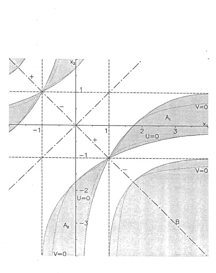
A i = { (x ,y ) : \y\ < ||a:| + 1, \x\ < 8 J, (2.2.8a)
Ao = { (x, y) ■ |y| < | | x | -f 1, |x| > 8 }, (2.2.86)
^3 = { ( x , y ) : \y\ > \ jxj - 1 }, and
(2.2.8c)
and write J — J] - J 2 + J?. where each J t is the integral over A
Note that g ( x , y ) is defined (at 2.2.1c) to be the difference between <p(x4- y) and the first terms of its Taylor series expansion about o(x). Thus
y) = £ y ‘V 3, (* + °y)' (2.2.9)
where 9 £ 0. 1 depends on x and y. We have
I
y* dnn{y)
iv < — - 1 - 1 2
-< v'n) - X 5 7( \ n < |JV| < ( | ; x | + 1)X/S ) }
£ 6n3 +
(|ix|
+ 1 ) 2 (2.2.10)(i) In .4] we use the crude estimate |d>l?)(;) < 0.6 for all 2, so
j \ < 0 . 1 f 6 n 3 + ( I N + 1 ) 6 „ 2 dx < c(bn 2 - 6 n 3 ) .
9jx|<8L J
(ii) For (x, y) € A 2 and 9 6 0,1; we have
I -+- 9y > jxj - jyj > * jxj - 1 > 3.
Now j f 3} (2:)j is decreasing as \ zj increases in \z\ > 3 (see Figure A.l in the Appendix), so it follows from (2.2.9) and (2.2.10) that
J 2 < C / \(p["^ ( I jxj - 1 ) 6n3 4- ( X + 1 ) f n2 d l < c(Sn2 4- f
23
(iii) To e s t i m a t e J 3 we p e r f o r m t h e i n t e g r a t i o n over x first, gi vi ng
J z < n \ / \ g { x , y ) \ d x d / j n(y) J | y I > 1 J 1 6 R
< n J ^1 + \y\ j \<p'[x)\dx + \ y 2 j \<t)"(x)\dx^J dfin (y)
< 3n j y 2d y n (y) d\y\>l
— obr,").
T h i s c o m p l e t e s t h e p r o o f of L e m m a 2.2.1.
Pr oof o f Le mma 2.2.2. T h e p r o o f is s i m i l a r t o t h a t of L e m m a 2. 2. 1. For \y\
e x p a n d g ( x , y ) t w o t e r m s f u r t h e r t h a n (2.2.9) t o give
9 ( x , y ) - i U ' V 31M - ^ y 4d>( , ! (.r) = Y‘2öy d>ir>) (x + Oy)
w h e r e 0G [0. L . T h e f u n c t i o n 6 ir': (z) is d e c r e a s i n g w i t h i n c r e a s i n g \z\ > 4, so t h e n o (;'*(x -f Oy). < j<^s ) ( jX! - 1) . T h u s , i n t e g r a t i n g (2.2.1 1) o v e r x G B we
G ( B . y)- iy3<J>
l3)(B)-- r k y ' 1 ^ 5 U P ° ' ' ’ ( - ) "* j
For y > 1 we i n t e g r a t e g(x. y) d i r e c t l y t o get
o ' 4' { X - 1 ) dx x ! > r.
= c\y\
G ( B . y ) = 4 > ( B - y ) - 4 > ( B ) y < i > ' ( B ) - W 2<J>"(B)
w h e r e B ■+ y = { x + y : x €. B }. T h e r e f o r e
G ( B , y) - W ( B ) < |y| 1 + <i>(B) - j t ' ( B ) < c\y\.
L e m m a 2. 2. 2 now follows by p u t t i n g y — - X / \ n in t h e e s t i m a t e ( 2. 2. 12) if
a n d in ( 2. 2. 14) if \X\ > ^ n, a n d tlien t a k i n g e x p e c t a t i o n s .
□
< 1 we
(2.2.11)
I if |x| > 5
h a v e
(2.2.12)
r>
(2. 2. 13)
(2. 2. 14)
A’ I < V' T ,
2.3. Q - d e t e r m i n i n g C la s s e s .
A class 5 of Borel sets B is said t o he Q - d t t t r m i n i n g (QD) if, for each X G £ 2,
24
lim inf
n —► oo
s u p ßGS \ Qn (B)\ + n 1/2
<$n > 0. (2.3.1)
We have s u p Be5 jQ n (B) = 0 ( 8 n ) (see 2.2.5). so 5 is QD if and only if s u p BeS \Qn (B)\ x Sn to ö ( r c ~ 1/2) for each \ G £ 2. Also, if the leading term expansion (2.2.2) holds for all B € 5, then S is CD if and only if 5 is QD.
The n -1 2 term in the numerator of (2.3.1) is a little unsatisfactory. We suspect t hat it is superfluous; that is whenever there exists X E C2 with
l i m i n f f S U p » » i9 " ( B ) l U o ,
n
* ° °V
<S ,
Jthen there is another random variable X ' G C2 for which (2.3.1) fails. Results later on in this section imply t h a t this is indeed the case for classes S of j ust one or two sets. However we do not have a proof for the general case.
If any s ubs et of a class 5 is Q D t h e n so is 5. In t hi s sense large classes are more likely to be QD t h a n small ones. Indeed t here is no hope of finding a single set B t o m ak e up a Q D class by itself.
T h e o r e m 2 .3 .1 . Xo singleton S — {FI} is QD.
However we also have:
T h e o r e m 2 .3 .2 . Fix r — 2.3 or 4. If <5>!r)( ß ) = 0 for each B G 5 then S is not QD. Therefore there exist infinite classes t h at are not QD. For example, we might take S to be the class of all intervals symmetric, about the origin so t hat (B) —0 for all B G 5.
It t u r n s out t h a t some d ou b l et s 5 = { ß ] , ß 2} are QD, and we cha r ac t e r i ze these. P u t
where
^ r s { B u B 2 ) Vrs{*] , j x ) dxidx-2 (2.3.2 a)
so that
25 O r . f S i . B j ) = <S>,r »(ßi)<I><f ' ( ß , ) - 4>'r ) ( ß 2)4>(f)( B 1). (2.3.2c). Also let
H( B i, B 2, y ) =
f f
h { x x, x 2, y ) dxAd x 2 (2.3.3a)X 2 £ 1 32** X i £ - ö i where
h { x u x 2, y ) = </>t3)(xi)y(a:2, y) - <£(3)( z 2)y(*i, y), (2.3.36) so that.
H ( B I , B , , y ) = 4><3> (B, )G( ß2,«,) - ^ ( ß j M ß j . y ) . (2.3.3c)
T h e o r e m 2 .3 .3 . (a) If '^23(^1 , # 2 ) = 0 or ^ 34 (5 i , B2) — 0 then the doublet S — { B \ . B 2j is not QD.
(b) Otherwise, S is QD i f and only i f
H ( B i , B 2, y ) ^ 0 for all y ^ 0. (2.3.4)
We have g(x, 0 ) = 0 for all j. so G ( ß , 0 ) - 0 for all sets B. and H ( B\ . B 2,0) — 0 for all B\ and B-2. Theorem 2.3.3(a) is a generalization of Theorem 2.3.2 for doublets 5.
Proofs. To show t h at a class 5 is not QD we must construct a particular distribution for the random variable X G C 2 so that (2.3.1) fails. Lemma 2.2.2 states t hat
!<?„(ß) + p „ 2< t"(ß )+ J6„34>(3|(B) - (fl) < c ( ^ , - i n6). (2.3.5)
Thus, if we can find X € C 2 such that the 6nj terms cancel out on the left-hand side of (2.3.5) for each ß € 5. and -f 6^5 = 0(6,,). then 5 is not QD. The following l emma provides a suitable family of distributions.
L e m m a 2 .3 .4 . Let a 2, a 3 and a4 be Real numbers with a 2 0. a 4 > 0 , and a 2 + 1 a31 + o A = 1. There exists a random variable X G L2. and a divergent sequence A o f positive integers. such that as n —> oc through A we have
f ni — cijfir, 4- o(Q,) for j = 2.3 and 4. (2.3.6a)
and
4 u + 6n r, i- n 1' " = o(6n ). (2.3.6b)
The proof of Lemma 2.3.4 is deferred until Section 2.4.
P ro o f o f Theorem 2.3.2. Take ar = 1 and the two other a3 = 0 in Le mma 2.3.4, and
let A' be the ensuing random variable. It follows immediately from Lemma 2.2.2 t ha t (2.3.1) fails for this X .
26
P ro o f o f Theorem 2.3.3. The case <t>^3^(B i) = ^ ' ^ ( F L ) = 0 is covered by The or em 2.3.2, so we may assume t h a t ^ 0 .
(a) Suppose first t h at ^ 2 3 ( ^ 1 , B 2) — 0. Put
b = 3 ^ ,,(jB1)/<T*(3)(jB1 ),
a-2 = 1/(1 + b ), 03 = - 6 / ( 1 + 6 ) , and a4 = 0.
These a3 satisfy the conditions of Lemma 2.3.4. so let X be the corresponding random
variable and let .V be the sequence there. Then, in view of Lemma 2.2.2, we have
(1 + M)Qn(B) '(B) t )M>|3»(B) '(*n)
for any Borel set B. as n —- oc through A . It follows immediately that Q n ( B \ ) = o( f n ). and t h at
( 1 + \ b \ ) ^ 3>{B,) Qn (B.2) - )S„ + o(K) o(6„)
as n —♦ oc through A . Therefore (2.3.1) fails ami 5 is not QD.
To deal with the case ^ 2.4(B) ■ Bo) = 0 we take
6 = 4>(4’( ß , ) 4 $ (3,( B,),
Qi = 0, 0 2 - 6/(1 4- 6 ). and a4 = 1/(1 -r ;6 ),
and proceed as above. □
(b) This is a bit more subtle.
(i) Suppose first t h at (2.3.4) holds. We show t h at
max \ Qn ( B 3) > e ( B] , Bo)bn . (2.3.7)
3 = 1 >2
27 It follows from Lemma 2.2.2 that
since 6n] < 6n2 and <5ns < Sn4. Thus it remains to show t h at
max \ Qn{ Bj ) \ > c ( B u B 2)(6n2 + <5n4). 3 = 1 > 2
In view of the estimates (2.2.12) and (2.2.14) we have
' £ y 4* 34( B i , £ 2) + 0 (y5) as y —> 0
(2.3.8)
H( Bl t B2,y)
\ y 2' ^2z ( B \ , B 2) T 0 ( y ) as y -» ±oo.
(2.3.9)
Now, by hypothesis, ^ 23 7^ 0 and 'L34 72 0, so H is the same sign as ^34 for small |y|, and H is the same sign as vL2o for large y . But H is a continuous function of y, which, according to (2.3.4), is non-zero except at y = 0. Therefore 'Loo and vLo4 must be of the same sign. Suppose first t h at they are both positive. It follows from (2.3.4) and (2.3.9) t hat
f c ( B \ , B-i)y4 for iy! < 1
H ( B „ B 2, y ) > ‘ (2.3.10)
{ for > 1,
S O
4>m (B,)CMB2) - 4>(3,(B2)<5„(B1)
t i E H l B i. ß 5. - .Y/ V” ) > f ( B „ B 2)(«n4 + i m ) - (2-3.11)
This implies (2.3.8). If ^03 and ^34 are both negative then the inequalities are just reversed in (2.3.10) and (2.3.11). so (2.3.8) still follows.
(ii) Next suppose that H ( B \ , B 2. yo) — 0 for some y() 7^ (). We use the following lemma to produce a random variable X G for which (2.3.1) fails.
L e m m a 2.3.5. Given yo,yi 7^ 0, there exist random variables Vu,T] G C 2, a sequence q n , and a divergent sequence X o f positive integers, such that all the following results hold asymptotically as n —> oc through X :
(a) ~ O n , ^ ‘ - O n - a n d n 1 “ = o(-j„);
(b) n E G { B , - ) \ ) j \ rn) = G ( B . y0) 4 (',y(> m ( B)
(c) n E G ( ß , - y , / v ^ ) = + o ( 7 „)
28 for any Bore] set B.
Lemma 2.3.5 is a special case of Lemma 2.4.2 which is proved in the next section.
Since & 3) { Bi ) ^ 0 we may define y] by the equation
G ( B , , yo) + l(Vo - 2y?)4>|3>(B,) = 0 . (2.3.12)
Suppose first t h a t y\ 0. We take A' to have induced measure | ( p o + p j ) , where p 0 arid pi are the probability measures induced by the random variables Yq and of Lemma 2.3.5. Note t h a t A' G C2. We have
( B i ) = n E G ( B 1, - X / y / f i )
= h i E G { B u - Y 0/ \ / n ) G { B \ , yo) -r 1 (y0’
- ^ nEG (Bi , —V i / v n )
"7n -
o(jn)
= ° ( l n )
as n —► oc through .V, in view of (2.3.12). Furthermore
<s><3|(Bi)q? (b2) o>(:i|(ß2)e„v UM
<J>l3)( ß , ) G ( ß 2.!/n) - 4>,3, ( ß 2 ) G ( ß „ ! / t , )(3) , ° f r n )
-
l B( B] . B i
• y o b * - r o ( q 7 i)= 0( 7 r j ,
so Q* ( B- 2) = o(7n) as n oc t hrough A . Since <S* 1 ) x q n and
n“ 1' 2 — o(7n ) as n —» oo through A . we see that (2.3.1) is false.
n
If yi = 0 then we take A” = Yq. It follows as above t ha t \ Qn [ B3) — 0(7 ^) as
29
2.4. C o u n t e r - e x a m p l e s .
To show t h a t a class S is not Q D we have to c o n s t r u c t a p a r ti c u l ar pr obabil i t y d is t ri b u t i o n for t he r a n d o m variable A so t h a t (2.3.1) fails. L e m m a s 2.4.1 and 2.4.2 below' present t wo families of d i s t ri b u t i o n s t h a t are useful in such cons t ruct i ons . Th e y are relat ed t o t he c o u n t e r - e x a m p l e on page 360 of Hall (1983).
L e m m a 2.4.1 has al ready a p p e ar e d as L e m m a 2.3.4, b ut we r e s ta t e it here for convenience. Recall t he definitions
2 + I ^n3 i + ^n4 = E | A “ 7(|A”| > \ / n ) j
+ n - V2e (.V3 7([JVI < v/H)}| + n “ 1E j A 4 7(|A| < y'n)},
h i = \ / Se { | A | / ( | A | > VS)}, and «„5 = » - 3/2E { | A j 5 /(!A| < y»)}
-L e m m a 2 . 4 . 1 . -L et a 2, a?, a n d a 4 be Real n u m b e r s w ith a-> > 0, a 4 > 0, a n d a 2 + «31 t a 4 = 1. There e x ists a r a n d o m variable A 6 £ 2. and a divergent sequence X o f p o s itiv e in te g e rs, such th a t as n —> oc through X we have
8nj — a76n — o(£n ) for j = 2 . 3 a n d - I , (2.4.1a)
and
h i -h : . + n r ' - = o(^„). (2.4.16)
Incidentally, thi s l emma shows t h a t any of t he t h re e t e r m s of bn may d o m i n a t e t h e o t h e r s a s y m pt o t i c a l l y (t ake t wo of the a ds to be zero). T h u s t here is no obvious way t o o bt ai n a si mpler sequence t h a n 8n which is of t h e s a m e precise order as 8n for all A e £ 2.
O u r second l emma includes L e m m a 2.3.5 as a special case.
L e m m a 2 . 4 . 2 . Given a 0 a n d 6 - ^ 0 there exist r a n d o m variables Va 6 C 2 and
Zb 6 £ 2w ith the following properties.
(a) T h ere is a sequence q n an d a divergent sequence X o f p o s itiv e integers such tha t
X On, f>n - On- aild 7) 12 = o(7n )
3 0
(b) If a function F( y) satisfies
and
IF( y) ~ ty* i £ c4y4 when \y\ £ 1
' F{y) < c2y 2 when y\ > 1
for some constants t, c4 > 0 and c2 > 0 , then
n E F ( - Y / \ n) = F { a ) d t a3 7 n + 0(7 «) and
i E F ( - Z / y / ^ ) = - 2 t b 3ln + o ( 7 n )
(2.4.2a)
(2.4.26)
(2.4.3a)
(2.4.36)
as n —» 00 through .V.
To get Lemma 2.3.5 put F(y) = G ( ß , y ) and / = 3>(S) ( # ) . Jn this case the estimates (2.4.2) follow from (2.2.12) and (2.2.14).
P ro of o f Lemm a 2.4.1. Suppose first t ha t a 3 > 0. Define functions
a 22 — (m — i)2y ~3 when 2 (rn~ F z < y < 2m2“ m (m > 3) A ( y ) = j °
M - y )
for other y > 0 when y < 0 ,
j 2a 3y 4 when 2771 1 < y < 2m ( m > 3) M y ) = \
( 0 for all other y.
( a 42mV 5 when 2m‘ m < y < 2m‘ ( m > 3) A ( y ) = \ 0 for other y > 0
(2.4.4a)
;2.4.46)
(2.4.4c)
and
/ 4( - y ) when y < 0 .
FlJ[m) = f y Vj ( y) dy for m £ 3 and j — 2.3 or 4.
J-2
< » " - i l *■2 2« ’ "
-Easy calculations show t h a t
/ 2
M y ) t M y ) + M y ) dy =
[2/M(M + AtsM
+ 2F24(m)m > 3
< 'S ( m a 2 log 2 4- a 3 + a 4)2 m‘ 42m < 1 m 3
since a 2 -j- a 3 + a 4 = 1. This also implies that
31
Therefore we may construct a fourth function r(y), bounded and with bounded support, such t h a t / ( y ) = / 2(y) + / 3(y) + /^ (y) 4- r(y) is a probability density function with / yf ( y) dy — 0 and / y 1 2 f ( y ) dy = 1. Let X be an absolutely continous random variable with this density.
Take .V to be the sequence n k = 2 2k~ (k > 0). In the following a symp t ot ic , equations we write n = n k and assume t h at k is so large t hat r(y) = 0 whenever
IyI > 2k = y/n. Note t hat all the moments of r(y) are finite. As k —> oo we have
«„1 = 2 k:E { | V | / ( | V | > 2 t=)}
— 2^ ^ ' 127
^,2
( ) +
Fizi™)+ 2
/*]4
(m)
m > k
2*‘‘ 2 a 22>- 2(m- 1)' 3a , 2 m > k
- 2m' + i<i42 “ 2m' + s,m
*„2 = ^ | 2 M " » ) 4 0 ( 2 - ' " , - " V) = 2a-ik2~k~ l o g 2 + 0 ( 2 -fc").
= 0 { 2 ~ k
»- k~
n3
m > k
2 ~ k
,-2 k~
Y . f » w + o ( i ) 7TJ < /c
^ 4 = 2 — ' ] T 2 f 44( m ) * 0 ( 2 m-) and
*n5 = 2— 3k ~
= 2 a 3A’2 _fc' log 2 + 0 ( 2 " * ' ) ,
= 2a.xk 2 ~ k log 2 + 0 ( 2 ~ k~).
{ Z L [ 2 ^ 2 ( w ) ^ Fzs(™) ~ 2Fr,.x( u
i < k
m < k
I E m < /c
| a 222m‘ 3 a 322T7,' ~ 2 - 2 a 422m 0 ( 1 ) } = 0 ( 2 - fc=).
Therefore 6n — 2k2 k ~ log 2 -f 0 ( 2 A~) and n 1 2 = 2 1 2 n r 2 ~ A;1 == o(6n ) as n —> oc through .V. The asymptotic equations (2.4.1) now follow immediately.
The case a 3 < 0 is handled similarly; instead of / 3(y) we use / 3 (y) — - f z { - y ) . □
Proof o f L e m m a 2.4.2. Choose mo > 5 so large t h a t 2 rn" < a < 2™" and
o - m , , ^ ,, 2m". Then let V =• Ya be a discrete r andom variable with atoms at
y m EE - a2rn of mass p n, = 2 “"'!m ~m for each rn > m 0,
and just two further atoms at y x and y2 of mass p \ and p 2 chosen so t hat ) F I 2. Similarly let Z = € C 2 have atoms at
32
and at 27 and z 2 of mass q} and q2. Take A to be the sequence { n k = 2 lk : k >
and put 7 n = = 2 ~ k' + k.
(a) Observe that
!Vk\ < \fn~k < | y * + i | lf « < 1, y/. - 1.1 < V n * < :y*| if ia !
and Tfc 1 \/^~k <'' 2fc+l •
f jai| < 1 then writing n = n k we have
& ~ £ V-mPm
= ? '
32 o - m 24m _ 2 2 — k~ — fc
= Ofan),
m> /c4 1 m > fc 4 1
'ns ~ 2 _ £ VraPm. - 2 - =
y
a 32m ~ - 2 c P ' 2 - k~ + k771,,<m<k mn < m< k
A'
n4 ^ ry — 2k~ £ VmPm 2 . ^
y
a 2 4 0 m ‘4
m ~ a 7 n4= - 2 a 37,
and
as n -» oc through .V. If o! > 1 then the corresponding results are
^ n ‘2 a b t i ) ^ n ? . ~ — a a n d 6 , l 4 — o ( 7 n )
-In any case. 6^ q n as n —» oc through A . We also have
<\?2 = ° ( 0 n). <\fs ~ 2637n and <$,f4 = 0(7 ,,).
so as n —* oc through A . Finally, note that - 1/2 o- A-- _ 0(7 ^) as A:
(b) Suppose that the function F( y ) satisfies the inequalities (2.4.2). Writing n
for k > m 0 -+ 1 we have
n E F ( - y / v 7 = 2 J ‘ : V F ( - y m - 2 k ' ) p m
m — 1,2 , m > m,
= 2“' y r(
£-ym - )Pr »2 Ir"
TTI = 1 . 2 Now, in view of (2.4.2)
22fc" y [ q - !/m2 - l7 + ((y m2 - t 1 )3 m — 1.2
Pm
C4 2 2/‘ ^ ( y m 2 A ) ‘ p m = 0 ( 7 n ) ,
m =■ 1,2
!2fc'| ]jT [ F (a 2 m2" fc=) - t ( a 2 TnZ ~ k ~ )
m 11< m < k — ]
,2 k
< c42 ZK ^ ( a 2 rn' ~ kZ) m I, < m< fc — 1
k~ \ 4 4 t) — 2 A'
Prn = C 4 a 2iy — l ft ^ .-) m ” 4 m _
m n < m < fc — 1
} ,
— > O C .
= ttfc
° ( 7 n )
33
2 2k \ F { a 2 rn2~ k" ) p J m > fc-t-1
< c22“ =
Y,
(“2 m !' * i V « = C!«! £ 2 m " •+ m _o(7n)-m > /c-f ] m > fc4 1
Ther efor e
n E F( - Y/ y / n) = 22k~ F{a)Pk + 22 * ' ] T * a32 m,I < m < fc —1
3 r ) 3 m~ — 3k ~
P m T C>(7n )
= F ( a ) 2 “ fc2 + fcT / a 32 - ,f2 2m + o(7 n )
m , t < m < k — 1
F ( a ) + i a 3 7n -+- o ( 7 n )
as n oo t h r o u g h .V. In t h e s am e way it is easy to show t h a t
n E F ( - 2 / v 4 ) = 22k'-]T + o(7n)
m n < m < k
= - / f t - v * 2 x i 2'n + °('i")
m n < m < A:
= -2/,637n - 0(7,,)
34
3. I n f i n i t e I n t e r v a l s .
3.1. I n t r o d u c t i o n a n d S u m m a r y .
In this chapter we consider classes S of infinite intervals, and characterize those that are convergence determining. Suppose t ha t
S = { ( —oc, x] : x G X } (3.1.1)
for some set X C R. Then An [S) = supieX Pn (x) - T^x)i , where P n (x) = P n {( —oo, x } is just the distribution function of S n /^/Xi. Thus we are interested in the rate of convergence of the distribution function Pn (x) to <I>(x) at particular points x e X .
It was shown in Section 2.2 t h a t a class S of intervals is convergence determining
X 6 C 2. Now Q n is an absolutely continuous signed measure, and Q n ( R) = 0, so
for all x € R. It follows t h a t the convergence determining nature of a class 5 of infinite intervals depends only on the endpoints x. and not on the individual types (( —oo,x , ( - o c . x ) , etc.) of the intervals. We may therefore restrict ourselves to classes S of the form (3.1.1).
Let us adopt a definition of Hall (1982), and say t hat X is a convergence determining set (CD set ) if the corresponding class { ( - o o . x , : x £ X } is convergence determining. We can write
if and only if it is Q-determining: t h a t is s u pB ,_5 Q n ( B) x to 0 ( n 1;/2) for each
Q n { ( - O C , x]} = Q n {(~OC,x)} = - Q n { X. OC) } = - Q n {(x,Oc)}
Q n (x) = Q rl{ ( - o c , x } = n E G ( x , - X/ y/ ' n), w here
G(x. y) = $ ( x - y) - 4>(x) - yo(x) - | y V ( x ) . (3.1.26)
The set X is CD if and only if
(3.1.3)
35
Theorem 2.3.1 implies that, no singleton X = {x} is CD. The case of doublets X = { x i , x 2} is covered by Theorem 2.3.3. but in the next section we present a simpler version of this theorem for the case of infinite intervals (Theorem 3.2.1). Section 3.3 goes on to consider the collection of all CD doublets ( x i , x 2) as a set in the Real plane. We prove t h at large areas of the plane correspond to doublets t hat are CD (Theorems 3.3.3, 3.3.5 and 3.3.6). In particular, any set of four distinct points must include a CD doublet, and so be CD itself.
Therefore the only remaining case is t h a t of triplets X — { x i , x2,1 3}. In Section 3.4 we characterize all such triplets as either CD or not CD, except for those lying on two specific surfaces in R°' (Theorem 3.4.1). These surfaces of triplets are the only sets X whose CD nature is unknown. Finally, in Section 3.5. we examine some aspects of the geometry of the collection of all CD triplets in R '.
3.2. C o n v e r g e n c e d e t e r m i n i n g d o u b l e t s .
Theorem 2.3.3 provides a complete characterization of those doublets 5 = { ( - o c . X ] , ( — o c , x 2; } t h at are CD. However a slight simplification is possible in this special case of infinite intervals. Put
H ( x i , T 2, y ) = / / ( ( - o c . x j j , ( - o c , x2j, y)
- 4>"{x i) G(x2, y) - <f>"{x2) G ( x u y), (3.2.1)
where G(x. y) is defined at (3.1.2b).
T h e o r e m 3 .2 .1 . (a) I f X = { x i , x 2} C { — \ 3.0. \ /3} then X is not CD.
(b) Otherwise, X is CD i f and only if
H (x j . x 2, y) = 0 for all y / 0. (3.2.2)
3G P r o o f o f Theorem 3.2.1. (a) Note t hat if { x i . x 2} C { - \ / 3 , 0 , \/3} then </^3) (x j) = 0 = <£>*3' ( x 2). Thus Theorem 3.2.1(a) follows immediately from Theorem 2.3.2.
(b) This is covered by Theorem 2.3.3(b) so long as t/;i 2 7^ 0 and t/ ’23 7^ 0, where
Vv* = 1p r e ( x 1 ^ 2 ) = 0 ( r , ( ^ l ) ^ ( 'S) ( X 2) - <>( r | ( x2)<A)(5) ( :rl )
-But the following lemma implies t h a t (3.2.2) fails if t/’i2 = 0 or t/; 23 — 0, so the theorem
is proved. □
L e m m a 3. 2. 2. I f { x j , x 2} { — \ / 3 , 0, v 3 } , and / / ( x 1. x 2 y) 7^ 0 for all y / 0, then ^ 1 2 ( ^ 1 , ^ 2 ) 0 2 3 ( ^ 1 , ^ 2 ) > 0 .
P ro o f o f Lem m a 3.2.2. In view of the form (3.1.2b) of G ( x , y ) , it is easy to see t hat
tf(*i5*2,y)
Ya y4V’23 -r j^Q —1—y Sp-24 -f 0 ( y Q). -i- as a c yti — » Q V\ y 2V12 + y p02 T O ( l ) as jyj -> oc.
Thus this lemma shows that if { x j , x 2} ^ { - v' 3.0. \ 3} arid (3.2.2) holds, then f / ( x ] , X2,y) takes the same sign for all y ^ 0.
We show first t h at t/q2 = V’2 3 — 0 is impossible. In this case we would have
0 = V 2 3 - 2i/>i2
= (f)11 [ x\ ) d>(3)( x 2) - 2o' (x2) - <£"(x2) o f?,(x,) - 2 0 , ( x 1)
= ( X 1 - x 2 ) d > " ( X 1 ) < p " ( X 2 ) .
(3.2.3)
where the last equality comes from Lemma A.2 in the Appendix. Now. by hypothesis, / /( . ) = H( x j , x 2, .) is certainly not identically zero, so the case <?"(xi) — o " ( x 2) — 0 (or Xi - x 2) is excluded. But if, say. ö " ( x ] ) = 0 ^ y " ( x 2). then it follows from y 12 = 0 t hat (p'(x1) = 0 as well. This is the required contradiction.
Thus if t ’i 2 — 0 then y 23 A 0 ; so / / takes the same sign as V’23 for small positive
and negative y (see 3.2.3). If also y u2 7^ 0 then II ~ yt/ !02 as y —> ± o c , so H takes
opposite signs for large positive and large negative y. But H is a continuous function of y, so all this contradicts (3.2.2). We have shown t h at t/’i2 — 0 implies y0 2 — 0 as