INFLUENCE OF MICROSTRUCTURE ON THE PROPAGATION OF FATIGUE CRACKS IN INCONEL 617

(1)

CRACKS IN INCONEL 617

by

Benjiman Michael Albiston

A thesis

submitted in partial fulfillment of the requirements for the degree of

Master of Science in Materials Science and Engineering Boise State University

(2)

(3)

DEFENSE COMMITTEE AND FINAL READING APPROVALS

of the thesis submitted by

Benjiman Michael Albiston

Thesis Title: Influence of Microstructure on the Propagation of Fatigue Cracks in Inconel 617

Date of Final Oral Examination: 10 July 2013

The following individuals read and discussed the thesis submitted by student Benjiman Michael Albiston, and they evaluated his presentation and response to questions during the final oral examination. They found that the student passed the final oral examination. Megan E. Frary, Ph.D. Chair, Supervisory Committee

Michael F. Hurley, Ph.D. Member, Supervisory Committee Clyde J. Northrup, Ph.D. Member, Supervisory Committee Richard N. Wright, Ph.D. Member, Supervisory Committee

(4)

This investigation was conducted as part of the requirements for the degree of Master of Science in Materials Science and Engineering from Boise State University. The material and instruments used in this investigation were provided or made available by the Department of Materials Science and Engineering at Boise State University and the Center for Advanced Energy Studies. This research was funded by the Idaho National Laboratory and the Department of Materials Science and Engineering at Boise State University, under the supervision of Dr. Megan Frary. I would like to acknowledge Dr. Megan Frary, as her guidance, support, and understanding made this thesis possible. In addition, the useful discussions and support provided by Dr. Mike Hurly were deeply appreciated. A special thanks to the faculty and staff at Boise State University for

support and assistance in all facets of this research. Finally, thank you to my parents who encouraged and supported my goals in obtaining a higher education.

(5)

Inconel 617 is a candidate material for use in the intermediate heat exchanger of the Next Generation Nuclear Plant. Because of the high temperatures and the

fluctuations in stress and temperature, the fatigue behavior of the material is important to understand. The goal of this study was to determine the influences of the microstructure during fatigue crack propagation. For this investigation, Inconel 617 compact tension samples, fatigue tested by Julian Benz at the Idaho National Laboratory, were obtained. The testing conditions included two environments at 650 °C (lab air and impure-He) and varied testing parameters including: loading waveform (triangular, trapezoidal), loading frequency (0.01, 0.05 Hz), and maximum stress intensity factor, Kmax (20, 25, 30

MPa√m). The value of Kmax had the greatest influence in the crack growth rate followed by the testing environment. In this study, electron backscatter diffraction was used in order to relate the crack path to the microstructure on the scale of microns. Using this information the crack was found to crack in the {001} family of planes and <001> to the <112> family of directions with the least propensity to propagate in the <111> family of directions. This supports that crack growth in Inconel 617 at 650 °C propagates with a ‘quasi-cleavage’ mechanism. Also in this study it was found that the character of fatigue crack deflections within a grain versus that at a grain boundary differs with statistical significance. Within a grain, the deflection angle had a unimodal distribution with a mean of 16° ±15°. The low angle of deflection suggests that the plane of highest stress is the highest influencing factor. Also, the deflections at the grain boundary were found to

(6)

for fatigue crack deflection. Though, the fatigue crack growth rate was found to be highly influenced by the testing atmosphere and loading parameters, they were found to have no statistical significance on the fatigue crack path on the microstructural level. At these testing conditions, the crack grew at a rate slow enough for the microstructure to have influence on its path, though it was still constrained to remain close to the plane of highest stress. Developing a deeper understanding of the influence of microstructure on fatigue crack propagation will support selection of materials and design of the

intermediate heat exchanger for the next generation nuclear plant.

(7)

ACKNOWLEDGEMENTS ... iv

ABSTRACT ...v

LIST OF TABLES ...x

LIST OF FIGURES ... xi

LIST OF ABBREVIATIONS ... xvi

CHAPTER ONE: INTRODUCTION ...1

1.1: Motivation for Research ...1

1.2: Research Objectives ...2

CHAPTER TWO: BACKGROUND INFORMATION ...3

2.1: Inconel 617 ...3

2.2: Fracture Mechanics ...4

2.2.1: Linear Elastic Fracture Mechanics ...5

2.2.2: Griffith Fracture Strength Theory ...6

2.3: Fatigue ...7

2.3.1: Fatigue Crack Character ...9

2.3.2: Factors Affecting Fatigue Crack Growth ...10

2.3.3: Fatigue Cracking in Inconel 617 ...12

2.4: Electron Backscatter Diffraction ...13

2.4.1: Interpreting EBSD data ...17

(8)

CHAPTER THREE: EXPERIMENTAL METHODS ...21

3.1: Specimen ...21

3.2: Fatigue Crack Growth Testing ...22

3.3: Microstructural Analysis...23

3.3.1: Specimen Preparation for EBSD Analysis ...23

3.3.2: EBSD Data Collection Procedure ...25

3.3.3: EBSD Data Cleanup Procedure ...26

3.3.4: Analysis of Direction of Crack Propagation ...29

3.3.5: Analysis of Change in Crack Propagation Direction ...31

CHAPTER FOUR: RESULTS ...33

4.1: EBSD Results and Statistics ...33

4.1.1: Bulk Microstructural Analysis ...44

4.2: Microstructural Characterization of Crack Propagation ...45

4.3: Change in Crack Propagation Direction ...50

4.4: Areas of Recrystallization ...53

CHAPTER FIVE: DISCUSSION ...57

5.1: Microstructural Influence in Fatigue Crack Propagation Direction ...57

5.1.1: The Modulus Effect ...59

5.1.2: Quasi-Cleavage ...61

5.2: Microstructural Influence in Fatigue Crack Deflection ...63

5.3: Factors That Influence Fatigue Crack Propagation in Inconel 617 ...64

5.4: Areas of Recrystallization ...66

(9)

CHAPTER SEVEN: FUTURE WORK ...70 REFERENCES ...71

(10)

Table 1. Chemical composition of Inconel 617 (wt. %) [3] ... 4 Table 2. Chemical composition of Inconel 617 used in this study. ... 22 Table 3. Mechanical testing parameters of each test segment of the two specimens. For

the trapezoidal waveform, the information in the frequency column is in the form: ramp up (s) - ramp down (s) - hold time at Kmax (s)... 23 Table 4. Length of crack analyzed and the number of grains the crack traversed. ... 33 Table 5. The analysis of variance, ANOVA, results for the testing parameters,

environment and deviation location ... 53 Table 6. The analysis of variance, ANOVA, results for the testing parameters, and

environment ... 65

(11)

Figure 1. The formation of intrusions and extrusions due to cyclic loading. The number of cycles increases from left to right. ... 8 Figure 2. Crack growth rate curve, the three regions of crack growth can be seen, with

region II having a linear growth rate predicted by the Paris Law. ... 8 Figure 3. Left: Backscatter Kikuchi patterns from Inconel 617. Right: Schematic of the

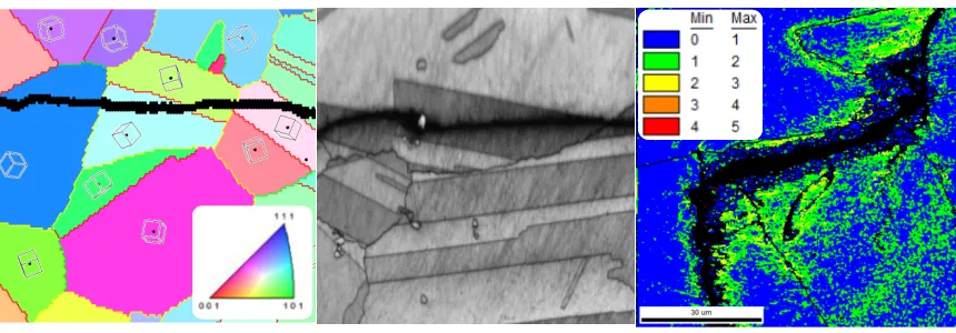
kossel cones with respect to the reflecting plane, incident beam, and the phosphor screen. ... 14 Figure 4. Using maps is the most common means to interpret EBSD data. Left: Inverse

pole figure (IPF) map. Each color represents a crystallographic

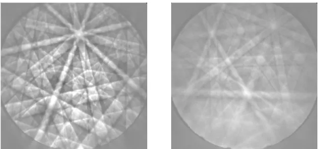
orientation as seen in the legend. Center: Image Quality (IQ) map. Each point represents the ‘quality’ of the electron backscatter pattern. Lighter shows higher quality while darker is lower. Right: Average misorientation Map. Each point is represented by its average misorientation from its neighbors from 0-5° ... 17 Figure 5. These are electron backscatter diffraction patterns (EBSP) obtained from

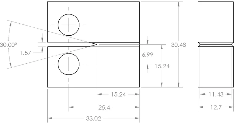
Inconel 617. Left: Shows a pattern with a high image quality. Right: Pattern with a low image quality. ... 18 Figure 6. Dimensions of the CT specimens received from the Idaho National Laboratory.

All dimensions are in millimeters unless otherwise noted... 21 Figure 7. Left: Image of the as-received sample from Idaho National Laboratory. Right:

The sample prepared for analysis after the groove is removed through mechanical polishing. ... 24 Figure 8. (a) Example of grain dilation. The white data point is not associated with either

grain. It is randomly assigned to a bordering grain. (b) Shows multiple iterations of grain dilation. Each point adjacent to a grain is assigned to that grain. This is repeated until all points are assigned. ... 27 Figure 9. IPF maps obtained during the data cleanup steps. (a) The raw data. (b) After the grain dilation and averaging cleanup steps. (c) Crack shown using the IQ threshold filtering. ... 28

(12)

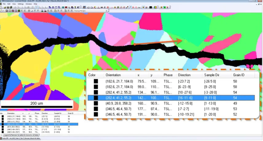
Figure 11. Screenshot of the EDAX/TSL OIM™ Analysis 6.2. The image includes an inverse pole figure map of a dataset post-cleanup. The arrow represents use of the OIM™ crystal direction tool, where the dot is the start within the grain in question and the arrow point is the terminus lining up the crack propagation direction within the grain. The orientation data is given below the map, enlarged in the dashed inset... 30 Figure 12. Screenshot of the EDAX/TSL OIM™ Analysis 6.2. The image includes an

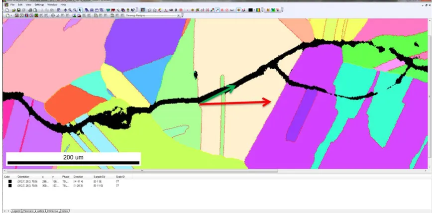
inverse pole figure map of a dataset post-cleanup. The arrows represents use of the OIM™ crystal direction tool, where the green arrow is the direction of crack propagation within the grain in question and the red arrow the direction the crack propagation changed from (both arrows need to be within the same grain to be comparable). ... 31

Figure 15. EBSD results for sample: lab air, Iteration 3 (Side 1). (Top) Image quality (IQ) map of the entire crack length where the lighter pixels have a higher the image quality. (Bottom Series) IPF map where the grain orientation is represented by colors seen within the unit triangle legend and the type of boundary is indicated by color. Yellow lines are general grain boundaries, green lines are CSL boundaries and red lines are Σ3 boundaries. ... 36 Figure 16. EBSD results for sample: lab air, Iteration 3 (Side 2). (Top) Image quality

(IQ) map of the entire crack length where the lighter pixels have a higher the image quality. (Bottom Series) IPF map where the grain orientation is represented by colors seen within the unit triangle legend and the type of boundary is indicated by color. Yellow lines are general grain boundaries,

green lines are CSL boundaries and red lines are Σ3 boundaries. ... 37 Figure 17. EBSD results for sample: impure-helium, Iteration 1 (Side 1). (Top) Image

quality (IQ) map of the entire crack length where the lighter pixels have a higher the image quality. (Bottom Series) IPF map where the grain

xii

Figure 13. EBSD results for sample: lab air, Iteration 1 (Side 1). (Top) Image quality (IQ) map of the entire crack length where the lighter pixels have a higher the image quality. (Bottom Series) IPF map where the grain orientation is represented by colors seen within the unit triangle legend and the type of boundary is indicated by color. Yellow lines are general grain boundaries, green lines are CSL boundaries and red lines are Σ3 boundaries. ... 34 Figure 14. EBSD results for sample: lab air, Iteration 1 (Side 2). (Top) Image quality

(13)

grain boundaries, green lines are CSL boundaries and red lines are Σ3

boundaries. ... 38 Figure 18. EBSD results for sample: impure-helium, Iteration 1 (Side 2). (Top) Image

quality (IQ) map of the entire crack length where the lighter pixels have a higher the image quality. (Bottom Series) IPF map where the grain orientation is represented by colors seen within the unit triangle legend and the type of boundary is indicated by color. Yellow lines are general grain boundaries, green lines are CSL boundaries and red lines are Σ3 boundaries. ... 39 Figure 19. EBSD results for sample: impure-helium, Iteration 2 (Side 1). (Top) Image

quality (IQ) map of the entire crack length where the lighter pixels have a higher the image quality. (Bottom Series) IPF map where the grain orientation is represented by colors seen within the unit triangle legend and the type of boundary is indicated by color. Yellow lines are general

boundaries. ... 43

(14)

Figure 24. Inverse pole figure unit triangles show the texture intensities for the impure-helium (top) and lab air (bottom) samples. ... 45 Figure 25. Crack propagation directions and planes for the impure-He sample. (a) Three

dimensional histogram showing the concentration of propagation

directions (b) Three dimensional histogram showing the concentration of crack propagation planes (c) Density histogram showing the concentration of propagation directions (d) Density histogram showing the concentration of crack propagation planes ... 46 Figure 26. Crack propagation directions and planes for the air sample. (a) Three

dimensional histogram showing the concentration of propagation

directions (b) Three dimensional histogram showing the concentration of crack propagation planes (c) Density histogram showing the concentration of propagation directions (d) Density histogram showing the concentration of crack propagation planes ... 47 Figure 27. The density histograms for each experimental parameter. ... 48 Figure 28. Angle of crack propagation for a random sample. (a) 3D and (b) 2D density

histogram showing the concentration of directions ... 49 Figure 29. IPF map showing examples of well-defined crack path changes (green circles) and those with less definition (red circles). Only a small selection of crack path deviations is marked... 50 Figure 30. Histogram of all crack propagation deflection angles for both samples. ... 50 Figure 31. Histogram of deflection angles occurring at (a) general grain boundaries (b)

Σ3 grain boundaries (c) combined grain boundaries and (d) within grain.

The lines in (c) and (d) are the probability density functions for the

dataset. ... 51 Figure 32. Recrystallization area 1 located in the impure-He sample with a Kmax of 30

MPa√m, triangular waveform, 0.5 r-ratio and 0.05 Hz loading frequency. (Left) IPF map of area of recrystallization. The grain boundary type is

represented as (yellow) general, (green) special CSL, and (red) Σ3

boundaries. (Right) Local misorientation map with blue representing 0-1° and red representing 4-5° of misorientation. Grain boundaries are shown as black lines. Black areas in both maps represent the crack and other areas of low image quality. ... 54

(15)

(Left) IPF map of area of recrystallization. The grain boundary type is

represented as (yellow) general, (green) special CSL, and (red) Σ3

boundaries. (Right) Local misorientation map with blue representing 0-1° and red representing 4-5° of misorientation. Grain boundaries are shown as black lines. Black areas in both maps represent the crack and other areas of low image quality. ... 55 Figure 34. Recrystallization areas 3 (top) & 4 (middle and bottom) located in the

impure-He sample. Area 3 has a Kmax of 25 MPa√m, triangular waveform, and 0.1 Hz loading frequency. Area 4 has a Kmax of 30 MPa√m, triangular

waveform, and 0.1 Hz loading frequency. ... 56 Figure 35. Above are images showing each analyzed crack path. The inset in the upper

right corner shows that at magnification crack propagation starts in mode II for the first few microns. ... 58 Figure 36. Density histogram of all crack propagation directions from both samples. .... 59 Figure 37. Density histogram of all data points collected from crack path direction

determination via EBSD with the anisotropic Young’s modulus contours of nickel overlaid. (Top) Crack propagation direction (Bottom) Crack propagation plane ... 60 Figure 38. Crack propagation angle away from the <112> family of directions for all

samples. ... 62 Figure 39. The fatigue crack growth rates for Inconel 617 at 650 °C. Image courtesy of

Julian Benz, Idaho National Laboratory. ... 65

(16)

ANOVA Analysis of Variance

ASTM American Society for Testing and Materials

ChI Chemical-assisted Indexing

CSL Coincident Site Lattice

CT Compact Tension

EBSD Electron Backscatter Diffraction EBSP Electron Backscatter Patterns

EDS Energy-dispersive X-ray Spectroscopy

FCC Face-centered Cubic

FIB Focused Ion Beam

INL Idaho National Laboratory

IPF Inverse Pole Figure

IQ Image Quality

OIM™ Orientation Imaging Microscopy

SEM Scanning Electron Microscope

VHTP Very High Temperature Plant

(17)

(18)

CHAPTER ONE: INTRODUCTION

1.1: Motivation for Research

In May 2005, congress passed the Energy Policy Act of 2005, which established as law that the U.S. Department of Energy shall establish a Next Generation Nuclear Plant project [1]. This act stated that the project should develop and design a prototype reactor that has the capabilities to produce both electricity and hydrogen. Today the production of hydrogen is reliant on technologies that yield greenhouse gases, which the lowering of is a driving factor in our increasing need for H2 [2]. Based on the above requirements, the Very High Temperature Reactor (VHTR) design was selected for the project. This would allow for the creation of electricity and hydrogen in a state-of-the-art, thermodynamically efficient manner without the creation of greenhouse gases [1]. However, the use of this technology introduces significant obstacles that need to be overcome before the project can be realized. One of the first considerations to be satisfied is the designed service life; this reactor is required to remain in service for 60 years. Therefore, understanding the interactions of the materials used in the manufacture of the plant with the environmental conditions is imperative. The data and models for current high-temperature alloys are inadequate and will be a significant focus of the project.

(19)

many metallic materials that are available today [1]. The high temperature incorporates significant mechanical and chemical mechanisms of degradation that must be understood and designed around. These include time dependent deformation (creep), cycle

dependent deformation (fatigue), and corrosion. These processes are greatly influenced by the microstructure of the material. Understanding these interactions and the long-term stability of the microstructure are paramount to the success of the overall Very High Temperature Reactor project.

1.2: Research Objectives

(20)

CHAPTER TWO: BACKGROUND INFORMATION

2.1: Inconel 617

The proposed candidate materials for the intermediate heat exchanger for the Next Generation Nuclear Plant are Inconel 617 and Haynes alloy 230. The operating

conditions for the plant present challenges that must be overcome in materials selection. This includes withstanding temperatures up to 950 °C in helium for up to 60 years. For a material to qualify for implementation, there must be enough data on the mechanical properties for model development and codification under the American Society of Mechanical Engineers Boiler and Pressure Vessel Code. Both of the aforementioned alloys possess properties that allow for high temperature service with a good combination of high-temperature strength and oxidation resistance. However, as compared to Inconel 617, alloy 230 is relatively new and even though preliminary data suggests it can

outperform Inconel 617, it does not have an established database of properties. This leads to Inconel 617 as the primary candidate material as it can be codified within the timeframe of the project [1].

(21)

molybdenum-rich within the matrix [3]. The alloy is typically purchased in the solution annealed condition, although precipitation of carbides can occur during service [6]. High temperature corrosion is combated by the inclusion of aluminum and chromium along with the nickel, all of which form passive layers on the surface of the material [3]. Passivation of the bulk material effectively reduces the rate of corrosion; however, oxidation still plays an important part in the mechanical properties such as the fatigue resistance of the material. The interaction of oxygen along grain boundaries, micro-cracks, and in the matrix can have a detrimental impact on the overall service life and cost [4, 7-9].

Table 1. Chemical composition of Inconel 617 (wt. %) [3]

Element wt %

Nickel 44.5 min.

Chromium 20.0-24.0

Cobalt 10.0-15.0

Molybdenum 8.0-10.0

Aluminum 0.8-1.5

Carbon 0.05-0.15

2.2: Fracture Mechanics

Whether engineering an automobile, plane, or nuclear reactor, it is important to understand how a structural component will endure during its service life. Basic material properties can be used to determine safe service load limits, but an understanding of fracture mechanics will give insight into the stresses that a material can carry, with and without defects. How long can the part last, with and without defects? What is the confidence in your above answers?

(22)

fracture mechanics developed as a result of World War II; failures of welded ships, gas-transmission lines, oil storage tanks, and pressurized cabin planes drove the need for research [10]. All structures contain defects such as voids, porosity, and surface defects introduced during manufacture and/or during the service life. These defects can be initiation points for cracks during cyclic loading. Fracture mechanics accesses the durability of materials and structural members that contain cracks or crack-like defects, determining at what loads cracks may grow [11, 12]. Understanding the fracture mechanics of a material and with the development of models, structures can be

manufactured to enhance a safe service life while saving the cost of “over-engineering.”

2.2.1: Linear Elastic Fracture Mechanics

Linear elastic fracture mechanics require linear-elastic behavior, which is usually only seen in brittle materials such as ceramics. However, it can be applied to ductile materials in the region near the crack tip. This allows for analysis of the elastic stress field near the crack tip, which is described by the stress intensity factor, K. At the crack tip, the model shows the stress as infinite and therefore neglected. The stress field near the crack tip in an infinitely extended plate is approximated by:

𝜎𝜎�11(𝑟𝑟,𝜑𝜑) =_{√2𝜋𝜋𝜋𝜋}𝐾𝐾𝐼𝐼 cos𝜑𝜑₂�1−sin𝜑𝜑₂sin3𝜑𝜑₂� (1)

𝜎𝜎�22(𝑟𝑟,𝜑𝜑) =_{√2𝜋𝜋𝜋𝜋}𝐾𝐾𝐼𝐼 cos𝜑𝜑₂�1 + sin𝜑𝜑₂sin3𝜑𝜑₂ � (2)

𝜏𝜏̃12(𝑟𝑟,𝜑𝜑) = 𝐾𝐾𝐼𝐼

√2𝜋𝜋𝜋𝜋cos 𝜑𝜑

2sin 𝜑𝜑 2cos

3𝜑𝜑

2 (3)

(23)

this model to be used, the geometry of the specimen and crack length must be incorporated:

KI =σ√πa Y (4)

where ‘a’ is the half crack length. The ‘I’ subscript denotes mode I loading, which is one of three possible loading geometries. Mode I is a load normal to the crack plane; mode II is in the direction of crack propagation; and mode III is perpendicular to crack

propagation but still in the crack plane. Finally, Y is a parameter, which is a function of specimen and loading geometry.

2.2.2: Griffith Fracture Strength Theory

Stability of cracks were first analyzed by Griffith in 1920 [13]. His postulate was that the stability of a crack under stress is a balance between the change in potential energy from the introduction of new crack surface and the introduced stress. Therefore, in order for a crack to propagate, the introduced stress at the crack tip must overcome the cohesive strength of the material and an increase in potential energy of the system.

To derive a generalized crack driving force using Griffith’s theory [13], consider again an infinite plate. It will have a determined thickness of B, with a crack through this thickness of length 2a, have a uniform stress in both the x and y directions, and be of an elastic material. The potential energy of the system can be described by:

U = U0−U𝑎𝑎+ U𝛾𝛾 (5)

where U is the potential energy of the system, 𝐔𝐔_𝟎𝟎 = potential energy of the system before introducing the crack, 𝐔𝐔_𝒂𝒂 = the decrease in potential energy due to deformation

(24)

formation of new crack surfaces. Using the relationships for 𝑈𝑈𝑎𝑎 and 𝑈𝑈𝛾𝛾 described by Inglis [14] in his 1913 paper the crack driving force can be found using:

𝐺𝐺 = 𝜋𝜋𝜎𝜎_𝐸𝐸2𝑎𝑎 (6)

where G is the elastic energy per unit area of crack surface made available for a small increment of crack extension.

2.3: Fatigue

It is important to understand what fatigue is and its mechanism. A system where a material is cyclically loaded at less than its tensile strength can lead to a weakening or catastrophic fracture, not preceded by a large plastic deformation [12].

There are three stages of damage evolution in the fatigue process: crack initiation, crack propagation, and catastrophic failure. Fatigue fracture starts at highly loaded positions within the material; the localized stress concentrations are often caused by notches, whether by design or defect. However, even if a component is “defect free,” a crack can be initiated by surface roughening caused by plastic deformation [12]. This is caused from dislocation movement at stresses below the yield strength. Under cyclic loading, the small plastic deformations accumulate and initiate a crack. Figure 1

demonstrates how the movement of dislocations in slip systems can forms notches in an otherwise defect free material. These act as initiation points for fatigue cracks.

(25)

continues until the crack growth rate is nominally less than 10-5 mm/cycles [15]. Region III shows that increasing stress will cause the crack growth rate to quickly increase, leading to the crack becoming unstable and the part failing. Within region II, the nominal crack growth rate is between 10-5 and 10-3 mm/cycle [15]. This region is most important as the crack growth rate can be described by the Paris Law [16]:

𝑑𝑑𝑑𝑑 𝑑𝑑𝑑𝑑⁄ =𝐶𝐶(Δ𝐾𝐾)𝑛𝑛 ₍₇₎

Figure 2. Crack growth rate curve, the three regions of crack growth can be seen, with region II having a

linear growth rate predicted by the Paris Law. ΔK (log) da /dN ( log) III II I No Crack Growth Steady Crack Growth 𝑑𝑑𝑑𝑑 𝑑𝑑𝑑𝑑=𝐶𝐶(Δ𝐾𝐾)𝑛𝑛 R ap id U n st ab le C ra ck G ro w th S lo w C ra ck G ro w th C rit ic al S tr es s I n te n sit y F ac to r, K IC C ra ck O p en in g T h re sh o ld , K Th Failure Slip bands

(26)

where 𝑑𝑑𝑑𝑑 𝑑𝑑𝑑𝑑⁄ is the crack growth rate per loading cycle and the right side of the equation

has the range of the stress intensity factor, ΔK, and the material constants ‘C’ and ‘n’.

This model can be used in design to allow for fatigue cracking within the service life of the part with minimal risk of premature fracture. However, other considerations need to be made in this simple model because of the high temperature environment of the next generation reactor. For example, oxygen transport and oxidation have been shown to greatly affect the fatigue properties of a material [17-23].

2.3.1: Fatigue Crack Character

Deformation of a material when under a mechanical load is either elastic and reversible or plastic, which results in non-reversible changes within its microstructure. The movement of dislocations within the slip systems of the material accommodates plastic deformation. In face-centered cubic (fcc) materials, such as nickel, the slip systems are the {111} family of planes and 〈11�0〉 family of directions.

The literature places fatigue cracks into two categories: short and long cracks [15, 24-26]. Short cracks can be further classified as microstructurally, mechanically, or physically short cracks [15, 26]. In microstructurally short cracks, the propagation rate is determined by interactions with the local microstructure [27]. The deformation zone ahead of the crack is relatively large compared to the crack length. As the crack

(27)

Crack propagation is divided into two modes. These are related to, but should not be confused with, the stages of crack propagation seen in Figure 2. The modes of crack propagation are also related to, but differ from, the modes of loading a specimen. In this description of crack propagation, it is assumed that the ‘loading mode’ is always Mode I, normal tensile stress. In Mode I crack propagation, seen in stage II crack growth, the crack runs within the plane of maximum normal stress. In Mode II, seen in stage I crack propagation, the crack runs in slip planes most conveniently oriented relative to the maximum shear stress, approximately 45° from the direction of the normal stresses [15, 27]. This dependence on the orientation of slip planes with in the grain makes Mode II propagation dependent on its crystallographic orientation. The mode of crack

propagation for microstructurally short cracks is mainly Mode II and the transition from Mode II to Mode I crack propagation helps define the transition to mechanically short cracks [26]. According to ASM, a crack is short so long as the radius of the deformation zone is greater than one-fiftieth of the crack length [15].

The evolution from physically short cracks to long cracks is defined by the complete development of plasticity-induced crack closure. Long cracks are typically greater than 0.5 mm in length and propagate in stage II type crack growth [15, 26]. Stage II crack growth occurs by transgranular fracture and the magnitude of the cyclic loading stress is of much greater influence than the average loading stress or microstructure [15, 26].

2.3.2: Factors Affecting Fatigue Crack Growth

(28)

(further described below and in Section 2.3.3). The types of mechanical loading conditions include the loading frequency, waveform, stress intensity factor, and stress ratio [17, 28-31]. It has been found in many studies that the environment including temperature [32-38] and atmosphere [18, 39-43] plays a critical role in fatigue crack propagation in nickel-based superalloys. Many aspects of the microstructure influence the fatigue properties of a material. Studies show that secondary phases [38, 44, 45], grain size [46], grain orientation [47-51], and grain boundary character [48, 52-56] play an important role in the fatigue properties of nickel-based superalloys.

(29)

K, influenced the number of slip systems activated during fatigue crack growth. In low K regions, only a single preferred slip system operated and the fatigue crack grew in a zigzag manner due to strain hardening [58]. In high K regions, two preferential slip systems operated simultaneously and the fatigue crack grew in a direction perpendicular to the loading axis [58].

Grain boundary character has also been shown to have influence on fatigue cracking. Li et al. [48] showed that grain boundaries with high interfacial energy tend to nucleate fatigue cracks sooner. In copper bi-crystals, it was found that cracks preferred to nucleate at high-angle boundaries [56]. In a study performed by Gao et al. [52], it was found that an engineered microstructure with a 40% increase of special boundaries, discussed later in this chapter, displayed only a marginal fatigue endurance increase

while a fine grained (1.3 μm) versus a coarse grain (15 μm) microstructure saw a ~7%

fatigue endurance increase. Grain boundaries were found to provide impedance to transgranular fatigue crack propagation; boundaries with higher misorientation tend to cause larger crack deflections [52].

2.3.3: Fatigue Cracking in Inconel 617

Inconel 617 is usually used in its solution annealed condition, but microstructural changes occur during its service life. Early on, chromium and aluminum oxide form on the surface, and long-term service will see inter- and intragranular carbides form [59, 60]. Also during aging, gamma prime forms in Inconel 617; this induces fatigue crack

(30)

determine the damage mode: at high strain rates fatigue crack propagation is

transgranular, changing to intergranular with lower rates [44]. Similar trends were seen with dwell times in trapezoidal waveform fatigue loading. Larger dwell times (over 1 minute) produced intergranular cracking while short dwell times produced transgranular cracks [44].

The environmental effects on the fatigue properties of Inconel 617 have also been investigated. Kim et al. [62] investigated high temperature aging in an impure-He atmosphere. They found that the room temperature ductility of Inconel 617 was gradually lost with aging. It was proposed that intergranular oxides below the surface oxide layer and the coarsening of carbides on the grain boundaries were the cause of the loss of ductility. With the loss of ductility, the fracture mode was predominantly

intergranular [62]. In a study performed by Totemeier and Tian [43], fatigue testing was performed in air, vacuum, and purified argon. In all environments, the introduction of a tensile hold period (trapezoidal waveform) reduced the fatigue life [43]. Fatigue lives were found to be longer in inert environments than in air [43].

2.4: Electron Backscatter Diffraction

Electron backscatter diffraction (EBSD) in the scanning electron microscope is increasingly used as a tool for characterizing the microstructure of engineering materials. This analysis technique allows for determination of microstructural information such as individual grain orientations, local texture, and phase identification, along with

information such as stored energy or presence of plastic deformation [63-71]. In 1928, Nishikawa and Kikuchi observed the first diffraction pattern in

(31)

were obtained on a recording film placed in front of the specimen. This early technique was dubbed “high-angle Kikuchi diffraction” and is the basis of today’s automated electron backscatter diffraction. Due to the wide spread availability of scanning electron microscopes (SEM) and today’s computing power, this simple technique that could only characterize single points in a material can be used today to produce data on a square millimeter of material with a resolution below a micron in just a few hours. Today, with the introduction of the duel beam SEM/focused ion beam (FIB), three dimensional models of materials can be made.

Electron backscatter diffraction is an invaluable analytical method. There are many other tools including but not limited to transmission electron microscopy (TEM), X-ray Photoelectron Spectroscopy (XPS), and Raman spectroscopy that can give similar information on the structure and/or chemical composition of the specimen. However, no other technique can characterize the macrostructure of the material with micro-precision.

Electron backscatter diffraction patterns, as seen in Figure 3, are produced on a phosphor screen by high-energy electrons diffracted from the interaction volume of the

Figure 3. Left: Backscatter Kikuchi patterns from Inconel 617. Right: Schematic of the kossel cones with respect to the reflecting plane, incident

beam, and the phosphor screen. Incident

(32)

electron beam from the SEM within the specimen [63, 70, 71]. The light colored Kikuchi bands seen in the figure are the result of the diffraction from a single crystal.

Intersections of the Kikuchi bands represent distinct zone axes. The relation between the incident electron beam, diffracting plane within the tilted specimen, and the phosphor screen is seen in the left image of Figure 3. In an electron backscatter diffraction (EBSD) experiment, the sample is placed in the SEM with a 70° tilt with respect to the incident electron beam. Electrons that interact with the material will be scattered toward the phosphor screen because of the sample tilt. The width of the line is developed from electrons passing on either side of diffraction point. This produces a cone, called a Kossel cone, which produces lines instead of the typical diffraction spots seen in TEM experiments. The Kikuchi pattern is the gnomonic projection of the lattice on a two dimensional surface. The center point of the incident electron beam on the surface of the specimen is the center of the related Kikuchi pattern. Edges of the Kikuchi band relate to diffraction from the same set of planes within the interaction volume of the beam.

Multiple theorems are needed to fully describe Kikuchi patterns. However, for basic crystallographic orientation determination, Bragg’s law will suffice. The angles between the Kikuchi lines correspond to the interplanar angles while the width of the band is related to interplanar spacing, dhkl.

2dhkl sin(θ) = n λ (7)

(33)

The spatial resolution of the electron backscatter diffraction is dependent on many variables including the specimen material itself. The resolution differs in the x and y axes, because the diffraction patterns are produced from the interaction volume of the electron beam, and the sample is tilted 70°. With the proper parameters, the spatial resolution of copper is better than 0.05 microns, using a tungsten filament or 0.02 microns with a field emission gun [63].

Indexing Kikuchi patterns developed from electron backscatter diffraction is similar to indexing a traditional diffraction pattern. The separation between two adjacent Kikuchi lines is analogous to the separation between two (hkl) diffraction spots.

Therefore, the Kikuchi lines can be indexed in much the same way. First, consider two different Kikuchi lines from the planes (h1k1l1) and (h2k2l2). The separations between their pairs of excess and deficit lines, p1 and p2, are in the ratio [73]:

p1

p2 =

�h₁2_+k 1 2_+l

1 2

�h22+k22+l22

(8)

The angle between two pairs of intersecting Kikuchi lines are also analogous to the angle between the corresponding diffraction spots, just as long the Kikuchi lines are not far from the center of the pattern [73]. Since the Kikuchi lines are a two dimensional representation of a three dimensional cone (Kossel Cone) emitted from the point of diffraction, the line will curve if too far from the center.

θhkl= sin−1_�λ

2a√h2+ k2 + l2� (9)

Using the ratio 𝑝𝑝1

𝑝𝑝2 and 𝜃𝜃ℎ𝑘𝑘𝑘𝑘 the orientation of the crystal can be determined from a

(34)

With today’s technology, computers perform automated indexing of up to 450 patterns per second. In order to detect and digitize the Kikuchi bands, a Hough transform is applied [74]. The now digitized bands are compared to a look-up table generated from the known material parameters. A voting scheme is used to determine which

crystallographic orientation or even which phase is currently producing the pattern [63, 75]. With this technology, what took days can take only a fraction of a second to complete.

2.4.1: Interpreting EBSD data

There are multiple means to extract meaning from EBSD data, including

displaying properties in the form of maps as seen in Figure 4. The most common is the inverse pole figure (IPF) map (the left most illustration). This map is made of individual color-coded points where each shows sample direction relative to the crystal reference frame. The legend is a unit triangle with a color designated for each point or

crystallographic direction. The use of the triangle is possible in cubic materials since the rest of the inverse pole figure shows redundant symmetrical points.

Figure 4. Using maps is the most common means to interpret EBSD data. Left: Inverse pole figure (IPF) map. Each color represents a crystallographic orientation

as seen in the legend. Center: Image Quality (IQ) map. Each point represents the ‘quality’ of the electron backscatter pattern. Lighter shows higher quality while darker is lower. Right: Average misorientation Map. Each point is represented by

(35)

A second type of map is an image quality (IQ) map. This displays the ‘quality’ of the electron backscatter pattern (EBSP), as seen in Figure 5, at each pixel the gray scale represents the relative quality of the EBSP, where black is the lowest and white is the highest. The quality can depend on many factors including surface defects and

microstructural elements, thus it is not comparable between multiple scans but can be used to identify features in the microstructure. Examples of features that can be identified on an IQ map are grain boundaries, precipitates, and differing dislocation densities. Because the electron beam has an interaction volume within the material being analyzed, as it approaches a grain boundary, EBSPs for the grains on either side are produced. This lowers the overall ‘quality’ of the displayed pattern, thus showing the grain boundaries on the map. Overall dislocation density is shown in a similar manner, instead of patterns from multiple grains being produced, the pattern is disrupted by interactions with the dislocations [76]. Thus, a higher dislocation density will lower the image quality. The quality of the diffraction patterns is not only affected by the crystal lattice, but also by the material itself. Elements with higher atomic numbers typically produce stronger patterns. Therefore, scans with multiple phases containing differing elements will show a contrast in the IQ map [71].

Figure 5. These are electron backscatter diffraction patterns (EBSP) obtained from Inconel 617. Left: Shows a pattern with a high image quality. Right: Pattern with

(36)

Average misorientation maps are a means to identify strain in the lattice of the material being investigated. Local variations in misorientation of the crystal are a good indicator of strain. Each point in this map represents the average misorientation between it and all of its neighboring points to a defined nearest neighbor. The values will be between 0 and 5 degrees as a grain boundary is defined as a misorientation greater than 5 degrees [63].

2.4.2: Grain Boundary Character

It was generally believed until the 1930’s that all grain boundaries were similar in nature and that an amorphous layer cemented individual grains together [77]. In the intervening years, a more sophisticated knowledge of grain boundaries has developed. The interfacial region between grains can have varying properties such as energy [77, 78], chemical reactivity [77, 78], and mechanical properties [77-79]. These properties are linked to the misorientation between the two grains. Description of this

(37)

boundary energies, which are comparable to low angle boundaries [83]. The latter boundaries can be described by the coincident site lattice model [82, 85]. This binary approach to grain boundary classification aides the researcher in simplifying the effects of high versus low-atomic mismatch grain boundaries.

The coincidence-site lattice (CSL) model allows for correlation of the special properties with the existence of a periodic well-ordered intergranular area or super lattice [86]. In this model, lattice points that are in common with both lattices are identified.

The CSL is characterized by the coincidence index (Σ), in which 1/Σ represents the

fraction of lattice points common to both lattices [86]. For example, the Σ3 twin

boundary has a misorientation of 60°, but one in three lattice points are common between the two grains. Though there is a high degree of misorientation, the high atomic

(38)

CHAPTER THREE: EXPERIMENTAL METHODS

3.1: Specimen

Specimens were received from the Idaho National Laboratory (INL). Fatigue crack growth testing had been performed at INL on each sample. The Inconel 617 specimens were received in the compact tension (CT) form with the dimensions given in Figure 6. The specimens were cut from a plate of Inconel 617 obtained from Thyssen

Krupp VDM USA Inc (Florham Park, NJ). The chemical composition of the plate from the certification sheet is given in Table 2. The plate conforms to the specification ASTM B 168-08 and is in the solution annealed condition.

(39)

Table 2. Chemical composition of Inconel 617 used in this study.

Element wt. %

Nickel 54.1

Chromium 22.2

Cobalt 11.6

Molybdenum 8.6

Iron 1.6

Aluminum 1.1

Titanium 0.4

Manganese 0.1

Silicon 0.1

Carbon 0.05

Copper 0.04

Sulfur < 0.002

Boron < 0.001

3.2: Fatigue Crack Growth Testing

The mechanical testing was performed by the INL. The tests were performed according to the ASTM E647-08 standard. Each sample was tested in a controlled environment where both atmosphere and temperature are held constant during the fatigue test. Each experiment uses multiple tests segments, given in Table 3, with varying parameters including Kmax, waveform, and frequency.

(40)

Table 3. Mechanical testing parameters of each test segment of the two specimens. For the trapezoidal waveform, the information in the frequency column is in the form: ramp up (s) - ramp down (s) - hold time at Kmax (s).

Specimen 1 (Lab Air Atmosphere; 650 °C)

Increment # Kmax Waveform Frequency (Hz)

1 20 Sine 1

2 25 Sine 0.5

3 25 Triangle 0.5

4 25 Sine 0.1

5 25 Triangle 0.1

6 30 Triangle 0.1

7 30 Triangle 0.05

8 30 Trapezoidal 10-10-10

Specimen 2 (Impure-He Atmosphere; 650 °C)

Increment # Kmax Waveform Frequency (Hz)

1 19 Triangle 1

2 20 Triangle 0.5

3 20 Triangle 0.1

4 20 Triangle 0.05

5 20 Triangle 0.01

6 25 Triangle 0.5

7 25 Triangle 0.1

8 25 Triangle 0.05

9 25 Triangle 0.01

10 30 Triangle 0.5

11 30 Triangle 0.1

12 30 Triangle 0.05

13 30 Triangle 0.01

3.3: Microstructural Analysis

3.3.1: Specimen Preparation for EBSD Analysis

(41)

120 grit SiC paper on a Buehler (Lake Bluff, IL) EcoMet® 3000 grinder-polisher. The right image in Figure 7 shows the sample with the groove removed and polished to a 600 grit finish. Though it is unseen to the naked eye, there is a 7-8 mm crack present on the surface of the sample in the right image. After removal of the machined grooves, the

sample preparation procedure includes grinding in steps between 120 to 1200 grit SiC papers. This is followed by a final polish in a Bueler (Lake Bluff, IL) Vibromet 2® vibratory polisher with 0.05 µm alumina slurry for 36 h. The extended vibratory polish time was used in lieu of a final electrochemical etch in preparation for EBSD analysis.

In order to increase the area for analysis, multiple replications of EBSD data were taken from each side of both samples. After each analysis, approximately 500 µm were removed from the sample surface with 120 grit SiC paper. The surface was then re-prepared and EBSD scans of the newly exposed crack were obtained.

After all of the data collection iterations were completed, the sample was broken in two pieces in order to expose the crack surface. This allowed for confirmation of the crack length data obtained during mechanical testing by comparing it to the “beach-marks” formed by the change of testing parameters between each test segment. This

Figure 7. Left: Image of the as-received sample from Idaho National Laboratory. Right: The sample prepared for analysis

(42)

procedure allowed for direct correlation between the location of a point in the EBSD data and the mechanical test parameters.

3.3.2: EBSD Data Collection Procedure

Electron backscatter diffraction (EBSD) analysis was performed on a JEOL (Peabody, MA) JSM-6610LV scanning electron microscope (SEM) equipped with an EDAX (Mahwah, NJ) Hikari XP EBSD camera and an EDAX (Mahwah, NJ) TEAM™ EDS Analysis System. The scans were performed at the Center for Advanced Energy Studies (CAES). The EBSD scans with simultaneous energy-dispersive X-ray

spectroscopy (EDS) were performed at 25 kV accelerating voltage, a step-size between 0.5-2 µm, and a scan area of approximately 300 µm x 1000-3000 µm. Scans were taken from the crack initiation point to its terminus. The data was collected and indexed using EDAX/TSL Orientation Imaging Microscopy (OIM™) Data Collection software version 6.2.

During the original data collection, a nickel phase material file was used for indexing, which allowed for the maximum data collection rate. The EBSD data was then rescanned using the Chemical-assisted Indexing (ChI) scan feature within the

(43)

3.3.3: EBSD Data Cleanup Procedure

Before analysis of the EBSD data can be performed, data points that were not properly indexed during data collection must be evaluated to determine whether they are part of the crack or if they should be included within an adjacent grain. This was

performed with the EDAX/TSL OIM™ Analysis software version 6.2. Two different approaches are used in determination of the crack location versus non-indexed data points. The built in cleanup algorithms included within the software were used.

The first cleanup algorithm used was the neighbor orientation correlation, which tests two conditions to determine if the orientation of a data point should be changed. The first condition compares each data point to its surrounding points determining if its orientation differs from its immediate neighbors. Depending on the cleanup level chosen (level 0-5), the data point must differ from all neighbors for level 0 to one neighbor for level 5. If the first condition is satisfied, then the algorithm compares the neighbors with each other to determine the numbers that have similar orientations within a tolerance. For level 0 all must have similar orientation, and for level 1, all but one must have similar orientations, up to level 5. If the two conditions are satisfied, the data point’s orientation is randomly changed to that of one of its neighbors, which satisfies both conditions. For the selected cleanup level, the lower levels are performed first. This study used up to three iterations of the level 3 neighbor orientation correlation cleanup.

(44)

same grain, the point’s orientation is changed to that of the majority grain. If not, the orientation is changed randomly to one of its neighboring grains. This algorithm can be performed in a single or multiple iterations, where in the latter the algorithm is repeated until each data point is assigned to a grain.

The cleanup procedure for the bulk microstructural analysis included up to three iterations of neighbor orientation correlation and a single iteration of grain dilation. For the crack propagation analysis, the grain dilation cleanup algorithm is changed to

multiple iterations and two additional cleanup steps are added. The multiple iterations of grain dilation allows for the areas represented within the crack to be included in the grain in which it traverses, which “re-connects” the grains in order to simulate the original microstructure. Figure 9 shows the steps from raw data to cleaned up data with the crack shown.

It is assumed that before fatigue testing the bulk microstructure was strain free, therefore, there would be little orientation change within a single grain. During bulk

Figure 8. (a) Example of grain dilation. The white data point is not associated with either grain. It is randomly assigned to a bordering grain. (b) Shows

multiple iterations of grain dilation. Each point adjacent to a grain is assigned to that grain. This is

repeated until all points are assigned. (a)

(45)

microstructural analysis, this was found to be true with only a small misorientation field located on either side of the crack. With this in mind, the single (average) orientation per grain cleanup algorithm, was used to simulate the pre-test microstructure. In this

algorithm all orientation measurements within a grain are averaged and then replaced with the average, resulting in the grain having a single orientation.

The final step in the cleanup for crack propagation analysis was to differentiate the points located within the crack from those located in the bulk microstructure. This was accomplished by making a new data partition in which an image quality threshold was used to separate the two types of points. Figure 10 contains a histogram of the image

Figure 10. Histogram of the Image Quality for an EBSD map. The black dashed line represents the location of the IQ

threshold.

250 μm

Figure 9. IPF maps obtained during the data cleanup steps. (a) The raw data. (b) After the grain dilation and averaging cleanup steps. (c) Crack shown using the IQ

threshold filtering.

Grain Boundaries

(46)

quality of each point in a EBSD map, which was used to determine the image quality threshold used for the new partition. The intersection of the tail at the lower image quality and the “normal” distribution was used for the threshold. The example in Figure 10 would have an image quality threshold of approximately 700.

3.3.4: Analysis of Direction of Crack Propagation

To determine the effect of microstructure on crack propagation direction, the path of crack propagation in relation to the microstructural orientation was measured. It is assumed that the crack is a two dimensional plane that is perpendicular to the surface of the sample. Therefore, the crystal direction tool in the OIM™ Analysis software was used to determine the direction of crack propagation with in the grain. The dataset was first cleaned with the multi-iteration grain dilation and grain averaging steps. Before analysis, a data partition was formed with an image quality threshold in order to differentiate the crack from the microstructure. With these steps complete, an inverse pole figure map was used in conjunction with the crystal direction tool. The starting point for the tool is alongside the crack within the grain in question and the terminus is a point that allows the vector to be parallel to the section of crack being analyzed, as represented by the orange arrow in Figure 11. This procedure is repeated for the entire length of the crack for each determinable straight section. In this study, 5,299 data points were obtained for analysis.

(47)

The data also includes information on the vector. The “sample direction” is the Miller indices for the direction of the crack within the sample reference frame, while the “direction” is the Miller indices within the reference frame of the grain

For analysis, the Miller indices for the crack propagation within the grain reference frame were converted to a point in inverse pole figure (IPF) space using Wolfram (Champaign, IL) Mathematica® 9.0. This allowed for visualizing the data in a unit triangle of an inverse pole figure where the direction of crack propagation is

represented by the position of the point and other attributes such as grain size, phase, or testing parameters which are represented by size and/or color of the point.

Figure 11. Screenshot of the EDAX/TSL OIM™ Analysis 6.2. The image includes an inverse pole figure map of a dataset post-cleanup. The arrow represents use of

the OIM™ crystal direction tool, where the dot is the start within the grain in question and the arrow point is the terminus lining up the crack propagation direction within the grain. The orientation data is given below the map, enlarged in

(48)

3.3.5: Analysis of Change in Crack Propagation Direction

To determine the influence of grain microstructure and boundaries in the deflection of the fatigue cracks, the second approach analyzed the change in crack propagation direction and the parameters present during deflection. Similar to the previous analysis, the OIM™ Analysis crystal direction tool was employed. However, this analysis focused on sections of the crack that had a definable direction before and after a direction change. To perform the analysis, two vectors were made for each viable data point, 776; such points were measured in this study. As seen in Figure 12, the first vector is parallel to the crack propagation after the direction change (green arrow), while the second is parallel to the crack propagation direction before the path change (red arrow). Both vectors must be in within the same grain for the data to be comparable even if the change in propagation direction occurs at a boundary. Data similar to the first

Figure 12. Screenshot of the EDAX/TSL OIM™ Analysis 6.2. The image includes an inverse pole figure map of a dataset post-cleanup. The arrows represents use of

the OIM™ crystal direction tool, where the green arrow is the direction of crack propagation within the grain in question and the red arrow the direction the crack

(49)

(50)

CHAPTER FOUR: RESULTS

4.1: EBSD Results and Statistics

Multiple sets of EBSD scans of each sample were obtained for analysis. The overall length of the crack in the impure-helium and lab air samples was 5.244 mm and 7.638 mm, respectively. Table 4 contains data on the length of the crack in each sample and the number of grains traversed. A total of 62.20 mm of overall crack length that traversed a total of 1,461 grains was investigated. This accounts for 64 hours of EBSD scan time.

Table 4. Length of crack analyzed and the number of grains the crack traversed.

Impure-He Lab Air Total

Length of Crack 31.65 mm 30.55 mm 62.20 mm

# of grains traversed 774 687 1461

33,314,134 data points & 64 hours of scan time

(51)

34

(52)

35

by colors seen within the unit triangle legend and the type of boundary is indicated by color. Yellow lines are general grain

(53)

36

(54)

37

(55)

38

represented by colors seen within the unit triangle legend and the type of boundary is indicated by color. Yellow lines are

(56)

39

(57)

40

(58)

41

(59)

42

(60)

43

(61)

4.1.1: Bulk Microstructural Analysis

Electron backscatter diffraction analysis offers a means to investigate the microstructural character of a material, including the average grain size, texture, and phase distributions. Figure 23 shows the grain size distributions, with twin boundaries excluded, of the impure-helium and lab air samples. Both samples have approximately the same distribution with an average grain diameter of 80 μm.

The texture analysis, Figure 24, of both the impure-helium and lab air samples shows a maximum texture intensity of 1.645 and 1.811, respectively. A texture intensity of 1.5 means that the texture has an intensity of 1.5 over that of a random distribution; therefore, the textures in both samples are weak.

The phase distributions of the samples illustrate that both the impure-helium and lab air samples are homogenous with little phase separation. There was a small amount of secondary phase, less than 1% of the area fraction. EDS analysis found that the secondary phase had a high concentration of titanium and EBSD subsequently indexed

Figure 23. Grain size distributions, with ∑3 grain boundaries excluded, of the impure-He and lab air samples.

(62)

the phase with high confidence as a cubic structure with the point group symmetry 𝑚𝑚3�𝑚𝑚. However, the resolution of either technique does not allow for determining if the

secondary phase is a titanium carbide or nitride as both have similar lattice parameters. Because of the low area fraction and slight interaction with crack propagation, the secondary phase is not considered in this study.

4.2: Microstructural Characterization of Crack Propagation

The first analysis performed was the direction of crack propagation through the microstructure. This data will allow insight into the effects of the experimental

parameters, environment, and microstructure in determining the path of fatigue cracks. Figure 24. Inverse pole figure unit triangles show

(63)

In Figure 25, the 2D and 3D unit triangle inverse pole figure density histograms for the impure-helium sample are found. In (a) and (c), the location of each square in the figure represents the direction in the grain parallel to crack propagation; while the color and/or height represents the concentration of data points for that direction. In (b) and (d), the squares within the unit triangle represents the concentration of crack propagation planes. In these plots, blue represents a lower relative count while red is a high relative count of points representing the crack propagation directions and planes. It is seen in the figures that the crack has less propensity to propagate in the [111] direction and the most in the

Figure 25. Crack propagation directions and planes for the impure-He sample. (a) Three dimensional histogram showing the concentration of propagation

directions (b) Three dimensional histogram showing the concentration of crack propagation planes (c) Density histogram showing the concentration of

propagation directions (d) Density histogram showing the concentration of crack propagation planes

(64)

[001] to [112] directions. It can also be seen that the (001) is the most likely crack plane. This same trend is found in the lab air sample as seen in Figure 26.

Similar results to that of the overall impure-helium and lab air samples were obtained when isolating testing parameters (Figure 27). In this figure each testing parameter is represented: the top row is the two waveforms (triangular and trapezoidal), the middle row is the frequencies (0.1 Hz and 0.5 Hz), and the bottom row is the three values for Kmax (20 MPa√m, 25 MPa√m, and 30 MPa√m). This is repeated for both crack direction and crack plane normal. A similar trend is seen those as in Figures 25-26, suggesting that the crack path at the microstructural level is influenced by the grain

Figure 26. Crack propagation directions and planes for the air sample. (a) Three dimensional histogram showing the concentration of propagation directions (b)

Three dimensional histogram showing the concentration of crack propagation planes (c) Density histogram showing the concentration of propagation directions

(65)

orientation and not the testing environment or parameters. In order to confirm that the above results are from the interactions of the crack with the microstructure and not an

(66)

artifact of the sampling procedure, a random dataset was collected. In this sampling, measurements from random vectors taken from multiple samples were obtained. Figure 28 contains this data and it can be seen that the directions are uniformly distributed showing the previous trends are a relevant result.

(67)

4.3: Change in Crack Propagation Direction

As the crack propagates through the sample, there are points where there is a defined change in direction (Figure 29). In this analysis, the angle of this deflection is assessed. In Figure 30, all crack deflection angles are displayed in a histogram. The most probable deflection angles are those below 20°.

The next step of this analysis was to determine if where the deflection occurred carries any significance. Three location types were investigated: those that occurred at

Σ3 special boundaries, at general boundaries, and within the grain. Other types of special boundaries were not included in this study due to their minimal occurrence and

interaction with the crack. An analysis of variance, ANOVA, was used to determine statistical significance of each deviation location. Four location types were defined for

500 µm

Figure 29. IPF map showing examples of well-defined crack path changes (green circles) and those with less definition (red circles). Only a small selection of crack

path deviations is marked

Figure 30. Histogram of all crack propagation deflection angles for both samples.

(68)

the statistical analysis, deviations: within the grain, at general grain boundaries, at Σ3 grain boundaries, and at all grain boundaries (Σ3 and general grain boundaries

combined). Figure 31 contains histograms for each location type investigated: parts (a)

through (c) are the general grain boundary, Σ3 grain boundary, and combined grain boundary deflection location types, respectively. Part (d) is the histogram for the deflections that occurred within the grains. The lines in parts (c) and (d) are the probability density functions for the datasets.

Performing an ANOVA with all the three unique location types (within grain,

general grain boundaries, and Σ3 grain boundaries) revealed a significant difference: F(2, 773) = 4.070, p = 0.017, where a lower p-value indicates a greater significance. It is customary to consider p = 0.05 or 0.01 as the cutoff, depending on the level of

Figure 31. Histogram of deflection angles occurring at (a) general grain boundaries

(b) Σ3 grain boundaries (c) combined grain boundaries and (d) within grain. The lines in (c) and (d) are the probability density functions for the dataset.

n = 149 General grain boundaries

n = 223 Σ3 grain boundaries

n = 372 Combined grain boundaries

n = 372 Within grain

(a) (b)

(69)

significance needed to be achieved [87, 88]. In order to determine which of the location types were significant in the ANOVA, a post-test was needed. Tukey’s honestly

significant difference test [87] determined that at a significance level of 0.05 the deviations within the grain verses at the Σ3 grain boundaries are significant. In other words, the deflections seen at Σ3 grain boundaries are statically different from those that occur within grains. At a significance of 0.1, the deviations within grain verses general grain boundaries are also determined significant, however, this is not high enough significance to consider relevant.

In the next ANOVA, the general grain boundaries and Σ3 grain boundaries are analyzed without the data for within the grain. It was found that there are no statistically significant differences as determined by one-way ANOVA (F( 1, 370 ) = 0.007 , p = 0.932). In other words, the deflection at grain boundaries is not statistically affected by the character of the grain boundary. With those results, the data for both types of grain boundaries were combined.

By comparing the within grain deviations to those at the combined grain