High dimensional real parameter optimization with teaching learning based optimization Pages 807-816 Download PDF

(1)

* Corresponding author.

Contents lists available at GrowingScience

International Journal of Industrial Engineering Computations

homepage: www.GrowingScience.com/ijiec

High dimensional real parameter optimization with teaching learning based optimization

Suresh Chandra Satapathya*, Anima Naikband K Parvathic

a_{Sr Member IEEE , ANITS, Vishakapatnam, India} b_{MITS, Rayagada,India}

c_{Centurion University of technology and management (CUTM), Paralakhemundi, India} A R T I C L E I N F O A B S T R A C T

Article history: Received 12 April 2012 Received in revised format 12 June 2012

Accepted June 22 2012 Available online 27 June 2012

In this paper, a new optimization technique known as Teaching–Learning-Based Optimization (TLBO) is implemented for solving high dimensional function optimization problems. Even though there are several other approaches to address this issue but the cost of computations are more in handling high dimensional problems. In this work we simulate TLBO for high dimensional benchmark function optimizations and compare its results with very widely used alternate techniques like Differential Evolution (DE) and Particle Swarm Optimization (PSO). Results clearly reveal that TLBO is able to address the computational cost issue for all simulated functions to a large dimensions compared to other two techniques.

Keywords:

High dimensional function optimization

TLBO

Differential evolution PSO

1. Introduction

Even though there is a huge amount of work dealing with global optimization, there are still not many powerful techniques to be used for dense high-dimensional functions. One of the main reasons is the high-computational cost involved. Usually, the approaches are computationally expensive to solve the global optimization problem reliably. Very often, it requires many function evaluations and iterations and arithmetic operations within the optimization code itself. For practical optimization applications,

the evaluation of f is often very expensive to compute and large number of function evaluations might

(2)

challenge to solve high dimensional problems with reasonably less function evaluations. Recently, a new optimization techniques based on teaching learning approach known as Teaching Learning based optimization (TLBO) (Rao et al., 2011) is reported to produce better results as regard to the convergence speed. Rao, et al (Rao et al., 2012) have simulated many constrained and unconstrained real parameter optimization problems. Rao and Patel (2012) described the elitist TLBO algorithm for solving complex constrained optimization problems. The authors had provided the complete details of TLBO algorithm regarding its algorithm-specific parameter-less concept and the effect of common control parameters such as elite size, population size and number of generations on the performance of

the algorithm. The points raised by Matej Črepinšek et al. (2012) were already addressed by Rao and

Patel (2012).

In this paper we have attempted to simulate TLBO for various benchmark problems with different dimensions ranging from 10 to 500 to establish the effectiveness of TLBO over very popular classical PSO and DE.

The rest of the paper is organized as follows. In section 2 , we explain TLBO in brief. Section 3 provides the benchmark functions, parameter settings and simulation results. The conclusion and future enhancement is discussed in Section 4.

2. Teaching–learning-based optimization

This optimization method is based on the effect of the influence of a teacher on the output of learners in a class. It is a population based method and like other population based methods it uses a population of solutions to proceed to the global solution. A group of learners constitute the population in TLBO. In any optimization algorithms there are numbers of different design variables. The different design variables in TLBO are analogous to different subjects offered to learners and the learners’ result is analogous to the ‘fitness’, as in other population-based optimization techniques. As the teacher is considered the most learned person in the society, the best solution so far is analogous to Teacher in TLBO. The process of TLBO is divided into two parts. The first part consists of the ‘Teacher Phase’ and the second part consists of the ‘Learner Phase’. The ‘Teacher Phase’ means learning from the teacher and the ‘Learner Phase’ means learning through the interaction between learners. In the sub-sections below we briefly discuss the implementation of TLBO.

2.1 Initialization

Following are the notations used for describing the TLBO:

: number of learners in a class i. e. “class size”

: number of courses offered to the learners

: maximum number of allowable iterations

The population is randomly initialized by a search space bounded by matrix of rows and

columns. The parameter of the learner is assigned values randomly using the equation

, , (1)

where rand represents a uniformly distributed random variable within the range (0, 1), and

represent the minimum and maximum value for parameter. The parameters of learner for the

generation g are given by

(3)

2.2 Teacher Phase

The mean parameter of each subject of the learners in the class at generation is given as

, , … … , , … … , (3)

The learner with the minimum objective function value is considered as the teacher for

respective iteration. The Teacher phase makes the algorithm proceed by shifting the mean of the learners towards its teacher. To obtain a new set of improved learners a random weighted differential vector is formed from the current mean and the desired mean parameters and added to the existing population of learners.

(4)

is the teaching factor which decides the value of mean to be changed. Value of can be either 1 or 2. The value of is decided randomly with equal probability as,

1 0,1 2 1 (5)

It may be noted here that is not a parameter of the TLBO algorithm. The value of is not given as

an input to the algorithm and its value is randomly decided by the algorithm using Eq. (5). After conducting a number of experiments on many benchmark functions it is concluded that the algorithm

performs better if the value of is between 1 and 2. However, the algorithm is found to perform much

better if the value of is either 1 or 2 and hence to simplify the algorithm, the teaching factor is suggested to take either 1 or 2 depending on the rounding up criteria given by Eq.(5).

If is found to be a superior learner than in generation , than it replaces inferior learner

in the matrix.

2.3 Learner Phase

In this phase the interaction of learners with one another takes place. The process of mutual interaction tends to increase the knowledge of the learner. The random interaction among learners improves his or

her knowledge. For a given learner , another learner is randomly selected . The th

i

parameter of the matrix in the learner phase is given as

(6)

D Algorithm Termination

The algorithm is terminated after iterations are completed.

Details of TLBO can be refereed in (Rao et al., 2012)

3. Benchmark Functions, parameter settings and Simulation results

(4)

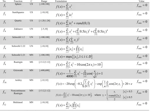
Table 1

Benchmark functions: C: Characteristic, U: Unimodal, M:Multimodal, S:Separable , N:Non-Separable

No.

Function Range C Formulation Value

1 f

Sphere US [-100,100] 2

1

( )

i D

i

f x x



  fmin 0

2 f

USSumSquares [-10,10] 2

1

( )

i D

i

f x ix



  fmin 0

3 f

Quartic US [-1.28,1.28] 4

1

( ) (0,1)

i D

i

f x ix rand



  fmin 0

4 f

UNZakharov [-5,10] 2 2 4

1 1 1

( ) ( 0.5 ) ( 0.5 )

i

D D D

i i

i i i

f x x ix ix

  

     fmin 0

5 f

Schwefel 1.2 UN [-100,100] 2

1 1

( ) D( i j)

i j

f x x

 

   fmin 0

6 f

UNSchwefel 2.22 [-10,10]

1 1

( ) D _i D _i

i i

f x x x

 

  fmin 0

7 f

Schwefel 2.21 MN [-100,100] _{( ) max}



_,1



i

f x  x  i D fmin 0

8 f

MSRastrigin [-5.12,5.12] 2

1

( ) D i 10cos(2 i) 10

i

f x x x

  

_{ }   _ fmin 0

9 f

Griewank MN [-600,600] 2

1 1

1

( ) cos( ) 1

4000 D D i i i i x

f x x

i

 

    fmin 0

10 f

MNAckley [-32,32] ₂

1 1

( ) 20exp 0.2 D i exp Dcos(2 i i 20

i i

f x x x e

D  n  

  _ _   _  _ _  _    min 0 f  11 f

Noncontinuous_Rastrigin MN [-5.12,5.12]

2 1

0.5 ( ) 10 cos(2 ) 10 , where _{(2 )}

0.5 2

i i

D

i i i _i

i

x x

f x y y y _round _x

x        _   _  _  min 0 f  12 f

MNMultimod [-10,10]

1 1

( ) D _i D _i

i i

f x x x

 

   fmin 0

Parameter settings

In all simulations of our work, the values of the common parameters used in each algorithm such as population size and total evaluation number were chosen to be the same. Population size is 50 and the maximum number fitness function evaluation is fixed as 100,000 for all functions. The other specific parameters of algorithms are given below:

PSO Settings: Cognitive and Social components, , are constants that can be used to change the

weighting between personal and population experience, respectively. In our experiments cognitive and social components are both set to 2 (Kennedy & Eberhart, 1995). Inertia weight, which determines how the previous velocity of the particle influences the velocity in the next iteration, is 0.5 (Kennedy & Eberhart, 1995).

DE Settings: In DE, F is a real constant which affects the differential variation between two Solutions

and set to F = 0.5*(1+ rand (0, 1)) where rand (0, 1) is a uniformly distributed random number within the range [0, 1]. In our simulation the value of crossover rate, which controls the change of the diversity

of the population, is chosen to be R = ( Rmax – Rmin) * (MAXIT–iter) / MAXIT where Rmax=1 and

Rmin=0.5 are the maximum and minimum values of scale factor R, iter is the current iteration number

and MAXIT is the maximum number of allowable iterations as recommended in (Storn & Price, 1997).

(5)

We have simulated each function with different dimensions for each algorithm. The range of dimensions is chosen from 10 to 500. The simulated results are presented in Table 2 to Table 5.

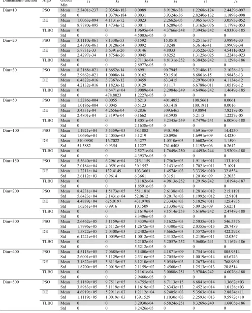
Table 2

Global Minimum values of Unimodal functions

Dimension/Function Algo Global Min

Dim=10 PSO Mean 2.3401e-237 2.0354e-183 0.0089 8.9128e-38 1.2268e-124 2.4429e-097 Std 0 1.0379e-184 0.0031 3.9324e-36 2.8240e-132 1.1898e-098 DE Mean 1.0063e-094 4.1131e-72 0.0023 2.2662e-05 7.0651e-075 3.0593e-052

Std 8.7780e-095 1.4734e-72 0.0011 1.6209e-05 1.3162e-076 1.1798e-053 TLBO Mean 0 0 1.9695e-04 4.3766e-248 7.3945e-242 4.8330e-185

Std 0 0 4.5003e-05 0 0 0

Dim=20 PSO Mean 3.1110e-061 8.1330e-53 0.1592 15.8510 5.2511e-37 3.9894e-33 Std 2.4790e-061 1.0128e-54 0.0092 7.8248 6.3614e-41 1.9909e-34 DE Mean 5.7731e-33 3.6391e-26 0.0146 4.8033 3.3522e-025 4.5411e-023

Std 2.4297e-34 1.8754e-26 0.0045 0.8252 1.3125e-025 1.2248e-023 TLBO Mean 0 0 2.7113e-04 8.8131e-252 6.3842e-242 1.1298e-186

Std 0 0 2.8977e-05 0 0 0

Dim=30 PSO Mean 8.2188e-021 1.6652e-14 0.6991 90.7945 3.2148e-13 2.1028e-13 Std 2.9862e-021 1.0008e-14 0.0162 50.1516 8.6861e-15 1.9843e-13 DE Mean 6.4822e-016 3.7367e-12 0.0459 63.3415 2.2970e-010 4.1134e-12 Std 4.2132e-016 1.1823e-12 0.0129 9.1117 6.6788e-011 1.0519e-12 TLBO Mean 0 8.6471e+04 3.9089e-04 2.2984e-249 4.6496e-242 1.4649e-185

Std 0 478.8023 1.2227e-05 0 0 0

Dim=50 PSO Mean 1.2286e-004 0.0055 3.6213 401.4852 108.5661 0.0061 Std 1.0186e-004 0.0045 0.5123 60.1418 100.1911 0.0016 DE Mean 3.4331e-04 4.2656e-04 0.2836 309.6465 19.8894 7.8218e-05

Std 2.4801e-04 2.3197e-04 0.1662 38.5938 5.2115 1.2227e-05 TLBO Mean 0 0 1.8051e-04 3.2345e-249 8.7479e-241 6.0080e-188

Std 0 0 2.1638e-05 0 0 0

Dim=100 PSO Mean 1.1921e+04 3.5359e+03 58.1882 940.1946 4.6916e+09 14.4230 Std 1.0696e+04 2.4055e+03 5.1219 20.0986 1.6991e+09 4.4230 DE Mean 510.0908 16.7022 6.4277 1.0510e+03 1.6602e+08 1.1590 Std 51.5882 0.9354 1.1227 761.6408 1.1192e+06 0.2612 TLBO Mean 0 0 2.5271e-04 1.7649e-250 4.4493e-244 3.9209e-188

Std 0 0 4.3937e-05 0 0 0

Dim=150 PSO Mean 5.5640e+04 6.2961e+04 215.1159 1.7563e+03 1.9115e+011 133.1091 Std 2.0184e+04 4.0591e+04 30.1552 2.1431e+02 1.7021e+011 7.1091 DE Mean 1.2211e+04 132.4149 103.3661 1.4574e+03 3.3339e+010 32.8534

Std 2.6112e+03 0.9614 6.3661 0.3151 1.2010e+09 2.2033 TLBO Mean 0 0 3.1182e-04 4.9813e-252 1.2919e-242 1.0194e-187

Std 0 0 1.8591e-05 0 0 0

Dim=200 PSO Mean 8.4231e+04 1.5173e+05 551.1816 2.6138e+03 1.2816e+012 215.1191 Std 5.6423e+04 2.1431e+04 52.0612 0.2017e+03 1.1992e+012 12.9101 DE Mean 4.4889e+04 625.0197 431.9708 2.3343e+03 5.1829e+011 125.4735

Std 1.6261e+04 0.9916 10.1509 2.1338e+02 5.0912e+09 5.6251 TLBO Mean 0 0 2.1619e-04 8.1514e-253 5.6169e-242 2.4748e-188

Std 0 0 8.3406e-05 0 0 0

Dim=300 PSO Mean 2.6462e+05 3.1159e+05 3.4339e+03 3.1622e+03 2.5035e+013 546.5376 Std 1.7996e+05 2.5112e+04 1.2672e+03 5.4300e+02 2.0355e+013 28.7489 DE Mean 1.5822e+05 2.0308e+03 2.2402e+03 3.6662e+03 1.5572e+013 422.2928

Std 6.1221e+04 1.0039e+02 1.0012e+02 2.3132e+02 1.2150e+011 12.0367 TLBO Mean 0 0 2.2102e-04 3.2057e-252 3.0600e-241 3.1167e-186

Std 0 0 5.5212e-05 0 0 0

Dim=400 PSO Mean 4.5115e+05 7.0685e+05 5.1400e+03 4.1871e+09 1.7541e+014 805.9514 Std 2.6001e+05 3.1129e+05 2.5316e+03 2.7055e+09 1.0019e+014 65.6746 DE Mean 3.1822e+05 3.6115e+03 6.1210e+03 5.0545e+03 1.2673e+014 768.9601

Std 1.8700e+05 2.0019e+02 2.1159e+02 2.4560e+2 1.2513e+013 20.8514 TLBO Mean 0 0 2.1161e-04 3.0088e-251 3.9784e-242 4.6076e-188

Std 0 0 2.9460e-05 0 0 0

Dim=500 PSO Mean 5.1189e+05 9.7511e+05 8.4755e+03 8.7113e+15 6.6841e+014 1.3662e+03 Std 3.8983e+05 3.1119e+05 1.1619e+03 2.6343e+13 2.4521e+014 1.0128e+03 DE Mean 4.6919e+05 5.2911e+03 1.2112e+04 6.2405e+03 5.3563e+014 2.8824e+11

Std 1.1119e+05 1.0019e+03 139.1529 1.1030e+03 2.2593e+013 9.5972e+10 TLBO Mean 0 0 3.2930e-04 6.5824e-251 8.3269e-240 1.6805e-186

(6)

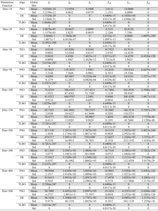
Table 3

Function Evaluations for Unimodal functions

Dimension/

Function Algo Global Min

Dim=10 PSO Mean 9.0360e-10 13.9294 0.1008 2.0133 14.0000 0

Std 5.2190e-12 4.0012 0.0179 1.1551 6.0000 0 DE Mean 3.7124e-29 0 0 4.4409e-15 6.1038e+04 0

Std 5.1460e-31 0 0 4.0117e-30 1.6360e+03 0

TLBO Mean 1.0648e-287 0 4.4409e-15 0 0

Std 0 0 4.0117e-30 0 0

Dim=20 PSO Mean 2.0070e-03 30.8437 0.0099 4.2335 45.0120 0

Std 1.1579e-03 3.8235 0.0019 2.1266 7.7501 0 DE Mean 2.6688e-7 1.7449e-06 0 2.6734e-13 0.0046 1.0097e-290

Std 1.0071e-7 6.4310e-07 0 1.0997e-13 0.0011 0

TLBO Mean 4.1992e-288 0 0 4.4409e-15 0 0

Std 0 0 0 4.0117e-30 0 0

Dim=30 PSO Mean 0.0156 65.8286 0.0144 10.7825 82.9134 0

Std 0.0052 12.6568 0.0137 2.8765 14.4239 0

DE Mean 0.0434 6.4506 7.4023e-12 2.0571e-07 14.4359 6.4520e-228 Std 0.0094 1.5867 1.4528e-12 7.7213e-8 1.0423 0

TLBO Mean 3.0154e-287 0 0 4.4409e-15 0 0

Std 0 0 0 4.0117e-30 0 0

Dim=50 PSO Mean 65.9625 139.2653 1.0561 14.2636 150.8362 6.6639e-310 Std 2.3144 7.2668 0.9861 0.3413 19.3266 0 DE Mean 4.6989 80.9887 8.3224e-04 2.9213e-02 54.6163 1.3271e-179

Std 0.1279 12.2012 6.0820e-04 1.0129e-02 6.1154 0

TLBO Mean 5.3387e-287 0 0 4.4409e-15 0 0

Std 0 0 0 4.0117e-30 0 0

Dim=100 PSO Mean 76.4219 306.6107 157.4211 16.7488 456.9036 2.3900e-282

Std 1.9252 87.4262 51.7580 1.1539 98.8347 0

DE Mean 41.9212 440.9707 2.2401 0.0049 308.4290 1.4817e-118

Std 0.9116 11.0371 0.6811 0.0016 12.5375 0

TLBO Mean 1.8258e-287 0 0 4.4409e-15 0 0

Std 0 0 0 4.0117e-30 0 0

Dim=150 PSO Mean 85.7225 641.8881 750.5357 18.2005 746.3139 5.7507e-278 Std 2.0108 34.6227 61.9606 0.5202 110.2351 0 DE Mean 59.4771 921.9111 58.0067 3.4694 680.4148 7.7559e-86

Std 0.4111 12.8201 9.9828 0.1291 45.7660 2.1599e-88

TLBO Mean 3.7261e-287 0 0 4.4409e-15 0 0

Std 0 0 0 4.0117e-30 0 0

Dim=200 PSO Mean 85.1136 1.2415e+03 1.3672e+03 18.5129 1.2025e+03 3.4823e-264 Std 1.4544 1.1749e+02 1.0071e+03 0.0829 2.5923e+02 0 DE Mean 69.6717 1.5051e+03 230.6390 12.6657 1.2266e+03 3.3532e-57

Std 0.5158 16.8913 30.7851 0.1516 515.1192 1.4103e-58

TLBO Mean 4.7261e-287 0 0 4.4409e-15 0 0

Std 0 0 0 4.0117e-30 0 0

Dim=300 PSO Mean 85.1305 2.2967e+03 1.4869e+03 18.7318 2.1001e+03 2.7262e-234 Std 5.0775 1.1907e+02 765.9498 0.0717 1.9468e+03 0 DE Mean 77.9417 2.7209e+03 1.1549e+03 16.2115 2.3121e+03 7.7160e-28

Std 0.8197 38.1902 1.0042e+03 0.3221 112.4358 3.0179e-29

TLBO Mean 2.2147e-287 0 0 4.4409e-15 0 0

Std 0 0 0 4.0117e-30 0 0

Dim=400 PSO Mean 90.9604 3.6349e+03 3.8054e+03 18.9043 2.9384e+03 3.4563e-183 Std 2.1917 3.9149e+02 1.0094e+03 0.0301 1.9212e+03 0 DE Mean 83.6613 3.9914e+03 2.4567e+03 17.6978 3.6283e+03 5.2065e+13

Std 0.5443 23.1615 2.2903e+03 0.2119 111.5880 7.3173e+07

TLBO Mean 2.2584e-287 0 0 4.4409e-15 0 0

Std 0 0 0 4.0117e-30 0 0

Dim=500 PSO Mean 94.7888 4.4452e+03 5.0997e+03 19.1034 4.3197e+03 5.4208e-108 Std 6.2757 1.0011e+3 73.1957 0.6034 2.1532e+02 2.1003e-124 DE Mean 86.1856 5.3880e+03 3.7707e+03 18.5342 4.9403e+03 1.2153e+43

Std 0.9176 48.1192 1.0019e+03 0.1017 542.1129 7.1556e+10

TLBO Mean 3.0154e-287 0 0 4.4409e-15 0 0

(7)

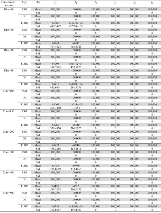
Table 4

Global minimum values for Multimodal Functions

Dimension/F

unction Algo FEs

Dim=10 PSO Mean 100,000 100,000 100,000 100,000 100,000 100,000

Std 0 0 0 0 0 0

DE Mean 100,000 100,000 100,000 100,000 100,000 100,000

Std 0 0 0 0 0 0

TLBO Mean 64665 6.3238e+04 100,000 100,000 100,000 100,000

Std 430.3467 8.7098e+03 0 0 0 0

Dim=20 PSO Mean 100,000 100,000 100,000 100,000 100,000 100,000

Std 0 0 0 0 0 0

DE Mean 100,000 100,000 100,000 100,000 100,000 100,000

Std 0 0 0 0 0 0

TLBO Mean 64945 64435 100,000 100,000 100,000 100,000

Std 704.4624 750.5343 0 0 0 0

Dim=30 PSO Mean 100,000 100,000 100,000 100,000 100,000 100,000

Std 0 0 0 0 0 0

DE Mean 100,000 100,000 100,000 100,000 100,000 100,000

Std 0 0 0 0 0 0

TLBO Mean 64795 8.6471e+04 100,000 100,000 100,000 100,000

Std 398.7805 478.8023 0 0 0 0

Dim=50 PSO Mean 100,000 100,000 100,000 100,000 100,000 100,000

Std 0 0 0 0 0 0

DE Mean 100,000 100,000 100,000 100,000 100,000 100,000

Std 0 0 0 0 0 0

TLBO Mean 64715 6.4909e+04 100,000 100,000 100,000 100,000

Std 455.6801 291.9371 0 0 0 0

Dim=100 PSO Mean 100,000 100,000 100,000 100,000 100,000 100,000

Std 0 0 0 0 0 0

DE Mean 100,000 100,000 100,000 100,000 100,000 100,000

Std 0 0 0 0 0 0

TLBO Mean 65065 1.3014e+03 100,000 100,000 100,000 100,000

Std 261.3460 7.3653 0 0 0 0

Dim=150 PSO Mean 100,000 100,000 100,000 100,000 100,000 100,000

Std 0 0 0 0 0 0

DE Mean 100,000 100,000 100,000 100,000 100,000 100,000

Std 0 0 0 0 0 0

TLBO Mean 64765 65240 100,000 100,000 100,000 100,000

Std 376.4970 200.6025 0 0 0 0

Dim=200 PSO Mean 100,000 100,000 100,000 100,000 100,000 100,000

Std 0 0 0 0 0 0

DE Mean 100,000 100,000 100,000 100,000 100,000 100,000

Std 0 0 0 0 0 0

TLBO Mean 64855 64840 100,000 100,000 100,000 100,000

Std 438.3256 455.8811 0 0 0 0

Dim=300 PSO Mean 100,000 100,000 100,000 100,000 100,000 100,000

Std 0 0 0 0 0 0

DE Mean 100,000 100,000 100,000 100,000 100,000 100,000

Std 0 0 0 0 0 0

TLBO Mean 65083 64980 100,000 100,000 100,000 100,000

Std 306.0689 334.4063 0 0 0 0

Dim=400 PSO Mean 100,000 100,000 100,000 100,000 100,000 100,000

Std 0 0 0 0 0 0

DE Mean 100,000 100,000 100,000 100,000 100,000 100,000

Std 0 0 0 0 0 0

TLBO Mean 64158 64965 100,000 100,000 100,000 100,000

Std 589.7228 306.0172 0 0 0 0

Dim=500 PSO Mean 100,000 100,000 100,000 100,000 100,000 100,000

Std 0 0 0 0 0 0

DE Mean 100,000 100,000 100,000 100,000 100,000 100,000

Std 0 0 0 0 0 0

TLBO Mean 64758 6.5069e+04 100,000 100,000 100,000 100,000

(8)

Table 5

Function Evaluations for Multimodal functions

Dimension/

Function Algo FEs

Dim=10 PSO Mean 100,000 100,000 100,000 100,000 100,000 100,000

Std 0 0 0 0 0 0

DE Mean 100,000 100,000 74575 100,000 6.1038e+04 100,000

Std 0 0 431.8004 0 1.6360e+03 0

TLBO Mean 100,000 16200 1.2633e+04 100,000 20225 1.6912e+05

Std 0 2.8036e+03 2.7029e+03 0 3.0704e+03 7.6285e+05 Dim=20 PSO Mean 100,000 100,000 100,000 100,000 100,000 100,000

Std 0 0 0 0 0 0

DE Mean 100,000 100,000 89300 100,000 100,000 100,000

Std 0 0 1.8816e+03 0 0 0

TLBO Mean 100,000 15540 9160 100,000 16925 1.7867e+04 Std 0 2.0651e+03 483.9493 0 4.3732e+03 818.0261 Dim=30 PSO Mean 100,000 100,000 100,000 100,000 100,000 100,000

Std 0 0 0 0 0 0

DE Mean 100,000 100,000 100,000 100,000 100,000 100,000

Std 0 0 0 0 0 0

TLBO Mean 100,000 15369 9200 100,000 1.9727e+04 3.3204e+05

Std 0 2.0516e+03 9.2968e+03 0 2.0449e+03 1.8693e+06 Dim=50 PSO Mean 100,000 100,000 100,000 100,000 100,000 100,000

Std 0 0 0 0 0 0

DE Mean 100,000 100,000 100,000 100,000 100,000 100,000

Std 0 0 0 0 0 0

TLBO Mean 100,000 11000 8875 100,000 13100 7050 Std 0 898.5703 315.6626 0 1.8865e+003 263.4930 Dim=100 PSO Mean 100,000 100,000 100,000 100,000 100,000 100,000

Std 0 0 0 0 0 0

DE Mean 100,000 100,000 100,000 100,000 100,000 100,000

Std 0 0 0 0 0 0

TLBO Mean 100,000 10090 9200 100,000 12550 3900 Std 0 790.1159 165.8312 0 1.2679e+03 64.1689 Dim=150 PSO Mean 100,000 100,000 100,000 100,000 100,000 100,000

Std 0 0 0 0 0 0

DE Mean 100,000 100,000 100,000 100,000 100,000 100,000

Std 0 0 0 0 0 0

TLBO Mean 100,000 9500 8875 100,000 10425 2620

Std 0 559.1529 193.9021 0 788.0282 162.3359

Dim=200 PSO Mean 100,000 100,000 100,000 100,000 100,000 100,000

Std 0 0 0 0 0 0

DE Mean 100,000 100,000 100,000 100,000 100,000 100,000

Std 0 0 0 0 0 0

TLBO Mean 100,000 9000 9200 100,000 10025 2280

Std 0 415.1161 0 0 470.6266 99.6546

Dim=300 PSO Mean 100,000 100,000 100,000 100,000 100,000 100,000

Std 0 0 0 0 0 0

DE Mean 100,000 100,000 100,000 100,000 100,000 100,000

Std 0 0 0 0 0 0

TLBO Mean 100,000 8700 8875 100,000 9325 1860

Std 0 300.1191 210.1912 0 832.2357 137.9655

Dim=400 PSO Mean 100,000 100,000 100,000 100,000 100,000 100,000

Std 0 0 0 0 0 0

DE Mean 100,000 100,000 100,000 100,000 100,000 100,000

Std 0 0 0 0 0 0

TLBO Mean 100,000 8600 8875 100,000 8950 1.4333e+03

Std 0 250.1106 115.1919 0 253.5463 47.8091

Dim=500 PSO Mean 100,000 100,000 100,000 100,000 100,000 100,000

Std 0 0 0 0 0 0

DE Mean 100,000 100,000 100,000 100,000 100,000 100,000

Std 0 0 0 0 0 0

TLBO Mean 100,000 8600 8875 100,000 8966 1.3656e+03

(9)

The fitness values and the number of function evaluations for six unmodal functions are shown in Table 2 and Table 4 respectively. Similarly, for multimodal functions it is shown in Table 3 and Table 5. The results are shown after 30 independent runs. The mean and standard deviations are calculated for obtained global minimum values and for the number of function evaluations in each algorithm with different dimensions.

Discussion of Results

In this work, all functions are run for 10 function evaluations (FFs) and the simulation is terminated

when it reached the maximum number of evaluations or when it reached the global minima value for each test function.

Fig. 1. Sphere Fig. 2. SumSquares Fig. 3. Quartic

Fig. 4. Zakharov Fig. 5. Schwefel 1.2 _{Fig. 6.}_{Schwefel 2.2}2

Fig. 7. Schwefel 2.21 Fig. 8. Rastrigin Fig. 9. Griewank

Fig. 10. Ackley Fig. 11. Noncontinuous Rastrigin Fig. 12. Multimod

From the Table 2 and 3 it is clear that, as the dimension increases, it is difficult for both PSO and DE to locate the global best position and the algorithm traps into local point, but it is not the case for TLBO. In other words, increasing dimensions will not effect for searching global best position in TLBO. From the Table 4 it can be verified that the number of FEs are considerably less for Sphere and SumSquare functions in TLBO compared to other two algorithms. Rastrigin, Noncontinous Rastrigin, Griwank, Multimod functions are finding optimal global values in TLBO with less FEs compared to DE and PSO

0 50 100 150 200 250 300 350 400 450 500 0 1 2 3 4 5 6x 10

5 _{Performance Calculation of Sphere Function}

Dimension Func ti on v a lu e PSO DE TLBO

0 50 100 150 200 250 300 350 400 450 500 0 1 2 3 4 5 6 7 8 9 10x 10

5 Performance Calculation of SumSquares Function

Dimension Fun c ti on v a lu e PSO DE TLBO

0 50 100 150 200 250 300 350 400 450 500 0 2000 4000 6000 8000 10000 12000 14000

Performance Calculation of Quartic Function

Dimension F u n c ti on v a lu e PSO DE TLBO

0 50 100 150 200 250 300 350 400 450 500 0 1 2 3 4 5 6 7x 10

14 _{Performance Calculation of Schwefel 1.2 Function}

Dimension F unc ti on v a lu e PSO DE TLBO

0 50 100 150 200 250 300 350 400 450 500 0 1000 2000 3000 4000 5000 6000

Performance Calculation of Rastrigin Function

0 50 100 150 200 250 300 350 400 450 500 0 10 20 30 40 50 60 70 80 90 100

Performance Calculation of Schwefel 2.21 Function

Dimension F u nc ti on v a lu e PSO DE TLBO

0 50 100 150 200 250 300 350 400 450 500 0 500 1000 1500 2000 2500 3000 3500 4000 4500 5000

Performance Calculation of Noncontinous Rastrigin Function

Dimension F u nc ti on v a lu e PSO DE TLBO

0 50 100 150 200 250 300 350 400 450 500 0 2 4 6 8 10 12 14 16 18 20

Performance Calculation of Ackley Function

Dimension Func ti o n v a lu e PSO DE TLBO

0 50 100 150 200 250 300 350 400 450 500 0 1000 2000 3000 4000 5000 6000

Performance Calculation of Griwank Function

0 50 100 150 200 250 300

0 500 1000 1500 2000 2500 3000 3500 4000

Performance Calculation of Zakharov Function

Dimension Func ti on v a lu e PSO DE TLBO

0 50 100 150 200 250 300

0 1 2 3 4 5 6 7 8x 10

-28 Performance Calculation of Multimod Function

(10)

particularly in increasing dimensions as shown in Table 5. In general all the functions experimented in our work, TLBO outperforms other two approaches. Fig. 1 to Fig. 12 presents the fitness curve of all tested functions against all algorithms.

It is clearly evident from above figures that TLBO is able to locate global minimum values for all functions even in high dimensions. However, PSO and DE fail to obtain optimal values even upto 100000 function evaluations. But on the other hand TLBO is able to find best global minimum values for all dimensions up to 500 within 100000 FEs. This fact establishes the ability of TLBO to optimize high dimension functions over other two well know optimization techniques DE and PSO.

4. Conclusion and future research

In this paper, a new optimization technique called Teaching-Learning based Optimization (TLBO) is implemented for solving high dimensional real parameter optimization benchmark functions. The results are compared with that of other two very popular optimization techniques known as Differential Evolution (DE) and Particle Swarm Optimization (PSO). From the simulation results, it is clearly noted that TLBO is a very powerful optimization technique in handling high dimension functions. Twelve benchmark functions belonging two unimodal and multimodal category are simulated with different dimensions ranging up to 500. In all functions, TLBO could able to locate global minimum function values with less number of function evaluations (FEs) compared to DE and PSO. This has clearly demonstrated the capability of TLBO as candidate to solve very high dimension industrial application problems. As a further research, it can be seen how TLBO address the multi-objective function optimization problems.

References

Becerra, R.L., & Coello, C.A.C. (2006). Cultured differential evolution for constrained optimization. Computer

Methods in Applied Mechanics and Engineering, 195, 4303–4322.

Črepinšek, M., Liu, S.H., & Mernik, L. (2012). A note on teaching–learning-based optimization algorithm.

Information Sciences, http://dx.doi.org/10.1016/j.ins.2012.05.009.

Holland, J.H. (1975). Adaptation in Natural and Artificial Systems, University of Michigan Press, Ann Arbor, MI.

Huang, F.Z., Wang, L., He, Q. (2007)An effective co-evolutionary differential evolution for constrained optimization.

Applied Mathematics and Computation, 186(1), 340–56.

Karaboga D, Basturk B. (2007). Artificial bee colony (ABC) optimization algorithm for solving constrained optimization problems. LNAI, 4529. Berlin: Springer- Verlag, 789–98.

Karaboga, D., & Akay, B. (2009). A comparative study of Artificial Bee Colony algorithm. Applied Mathematics and

Computation, 214, 108–132.

Kennedy, J., & Eberhart, R.C. (1995). Particle swarm optimization. IEEE International Conference on Neural

Networks, 4, 1942–1948.

Mezura-Montes, E., & Coello, C.A.C. (2005). A simple multi-membered evolution strategy to solve constrained optimization problems. IEEE Transactions on Evolutionary Computation, 9(1), 1–17.

Price, K., Storn, R., & Lampinen, A. (2005). Differential Evolution a Practical Approach to Global Optimization.

Springer Natural Computing Series.

Rao, R.V., Savsani, V.J., & Vakharia, D. P. (2011). Teaching–learning-based optimization: A novel method for

constrained mechanical design optimization problems. Computer-Aided Design, 43, 303–315.

Rao, V.J., Savsani, V.J., & Balic, J. (2012). Teaching learning based optimization algorithm for constrained and

unconstrained real parameter optimization problems. Engineering Optimization,

DOI:10.1080/0305215X.2011.652103.

Rao, R.V., & Patel, V. (2012). An elitist teaching-learning-based optimization algorithm for solving complex

constrained optimization problems. International Journal of Industrial Engineering Computations, 3, 535–560.

Storn, R., & Price, K. (1997). Differential evolution – a simple and efficient heuristic for global optimization over

continuous spaces. Journal of Global Optimization, 11, 341–359.

Zavala, A.E.M., Aguirre, A.H., & Diharce, E.R.V. (2005). Constrained optimization via evolutionary swarm

optimization algorithm (PESO). In: Proceedings of the 2005 Conference on Genetic and Evolutionary