Comparison of Nonlinear Filtering Methods for Battery State of Charge Estimation

University of New Orleans University of New Orleans

ScholarWorks@UNO

ScholarWorks@UNO

University of New Orleans Theses and

Dissertations Dissertations and Theses

Summer 8-13-2014

Comparison of Nonlinear Filtering Methods for Battery State of

Comparison of Nonlinear Filtering Methods for Battery State of

Charge Estimation

Charge Estimation

Klaus Zhang

[email protected]

Follow this and additional works at: https://scholarworks.uno.edu/td

Part of the Signal Processing Commons, and the Systems and Communications Commons

Recommended Citation Recommended Citation

Zhang, Klaus, "Comparison of Nonlinear Filtering Methods for Battery State of Charge Estimation" (2014). University of New Orleans Theses and Dissertations. 1896.

https://scholarworks.uno.edu/td/1896

This Thesis is protected by copyright and/or related rights. It has been brought to you by ScholarWorks@UNO with permission from the rights-holder(s). You are free to use this Thesis in any way that is permitted by the copyright and related rights legislation that applies to your use. For other uses you need to obtain permission from the rights-holder(s) directly, unless additional rights are indicated by a Creative Commons license in the record and/or on the work itself.

Comparison of Nonlinear Filtering Methods for Battery State of Charge Estimation

A Thesis

Submitted to the Graduate Faculty of the University of New Orleans

in partial fulfillment of the requirements for the degree of

Master of Science in

Engineering Electrical Engineering

by Klaus Zhang

B.S. Pennsylvania State University, 2011

Dedication

Acknowledgments

First and foremost, I would like to thank my thesis advisor Dr. Huimin Chen. His assistance and guidance on this project have been invaluable. He has inspired me to strive towards academic success and fulfilling my goals. My accomplishments over the past few years would not have been possible without his help.

I would also like to thank the other members of the defense committee, Dr. Vesselin Jilkov and Dr. Rasheed Azzam, for giving me valuable feedback on this project. I thank them for their support during my time at UNO.

Table of Contents

Abstract ii

List of Figures v

List of Tables vi

Acknowledgments vii

Dedication viii

Chapter 1

Introduction 1

1.1 Electrical Characteristics of Rechargeable Batteries . . . 2

1.2 Battery Models . . . 4

1.2.1 Electrochemical . . . 5

1.2.2 Computational Intelligence . . . 5

1.2.3 Analytical . . . 6

1.2.4 Stochastic . . . 8

1.2.5 Electrical-Circuit . . . 10

1.2.6 Evaluation . . . 12

1.3 Nonlinear Filtering Methods . . . 13

1.3.1 Extended Kalman Filter . . . 17

1.3.2 Unscented Kalman Filter . . . 18

1.3.3 Cubature Kalman Filter . . . 22

1.3.3.1 Third-Order CKF . . . 22

1.3.3.2 Fifth-Order CKF . . . 23

1.3.4 Statistically Linearized Filter . . . 25

2.2 Discretization of System Dynamics . . . 39

2.3 Simulation Setup . . . 43

2.4 Filtering Setup . . . 49

Chapter 3 Filtering Results 51 3.1 Performance Measures . . . 51

3.2 Sampling Period of 30 Seconds . . . 53

3.3 Sampling Period of 150 Seconds . . . 58

3.4 Sampling Period of 300 Seconds . . . 62

Chapter 4 Discussion 66 4.1 Summary . . . 66

4.2 Future Work . . . 67

Bibliography 69

List of Figures

2.1 Electrical-circuit battery model. . . 29

2.2 Loads to (a) discharge and (b) charge the battery. . . 32

2.3 Modeling of thermal noise in resistances as voltage sources in series with the resistances. . . 34

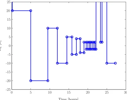
2.4 Input loadRL on the battery. . . 46

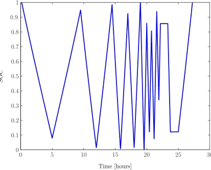
2.5 True SOC for one run due to input load. . . 47

2.6 Noisy measurementV_cell for one run. . . 48

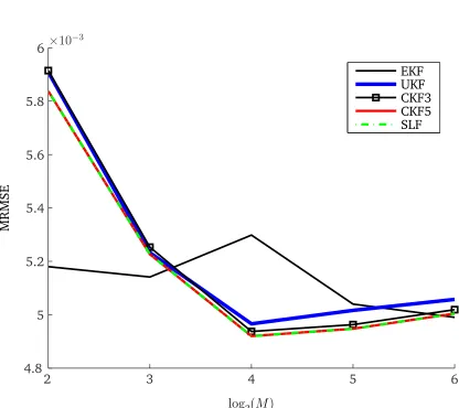
3.1 MRMSE of SOC estimation for Ts = 30 seconds as a function of number of integration steps M. . . 55

3.2 RMSE of SOC estimation forTs = 30seconds andM = 4. . . 56

3.3 RMSE of SOC estimation forTs = 30seconds andM = 64. . . 57

3.4 MRMSE of SOC estimation forTs = 150seconds as a function of number of integration steps M. . . 59

3.5 RMSE of SOC estimation forTs = 150seconds andM = 16. . . 60

3.6 RMSE of SOC estimation forTs = 150seconds andM = 256. . . 61

3.7 MRMSE of SOC estimation forTs = 300seconds as a function of number of integration steps M. . . 63

3.8 RMSE of SOC estimation forTs = 300seconds andM = 64. . . 64

List of Tables

1.1 Summary of relevant characteristics of various battery model types. 12

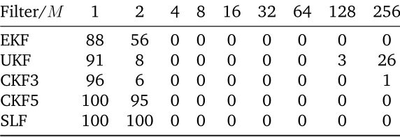
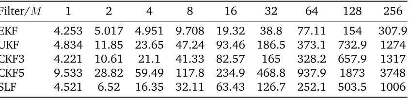
3.1 Number of divergences in 100 Monte Carlo runs forTs = 30seconds as a function of number of integration stepsM . . . 53 3.2 Filtering time in seconds for 100 Monte Carlo runs forTs= 30

sec-onds as a function of number of integration stepsM . . . 54 3.3 Number of divergences in 100 Monte Carlo runs forTs = 150

sec-onds as a function of number of integration stepsM . . . 58 3.4 Filtering time in seconds for 100 Monte Carlo runs forTs= 150

sec-onds as a function of number of integration stepsM . . . 58 3.5 Number of divergences in 100 Monte Carlo runs forTs = 300

sec-onds as a function of number of integration stepsM . . . 62 3.6 Filtering time in seconds for 100 Monte Carlo runs forTs= 300

Abstract

In battery management systems, the main figure of merit is the battery’s SOC, typically obtained from voltage and current measurements. Present estimation methods use simplified battery models that do not fully capture the electrical characteristics of the battery, which are useful for system design. This thesis studied SOC estimation for a lithium-ion battery using a nonlinear, electrical-circuit battery model that better describes the electrical characteristics of the battery. The extended Kalman filter, unscented Kalman filter, third-order and fifth-order cubature Kalman filter, and the statistically linearized filter were tested on their ability to estimate the SOC through numerical simulation. Their performances were compared based on their root-mean-square error over one hundred Monte Carlo runs as well as the time they took to complete those runs. The results show that the extended Kalman filter is a good choice for estimating the SOC of a lithium-ion battery.

Chapter

1

Introduction

Batteries, particularly rechargeable ones, are used extensively in daily life. They

provide the energy for such electrical systems as communication, automotive, and

renewable power systems. In order to design for and operate these systems, an

accurate battery model and a means of simulating the model efficiently are needed.

For example, modern battery charge and health management schemes use

high-fidelity battery models to track the state of charge (SOC) and state of health (SOH);

this information is then used to predict and optimize the runtime of the battery.

However, widely-used chemical batteries have nonlinear capacitive effects, which

require the use of a nonlinear filter for accurate prediction of their states in the

presence of noise. This thesis explores one possible solution to this problem by

choosing an appropriate battery model and testing the accuracy and speed of

various nonlinear filters in determining the SOC through simulation. Note that

only filters using point-based numerical approximation methods were studied, as

opposed to those using density-based methods. See [1] for more information about

the differences between various numerical approximation methods in relationship

1.1

Electrical Characteristics of Rechargeable

Batter-ies

A high-fidelity battery model has to accurately reproduce the various characteristics

of a battery. Most models keep track of the total capacity and SOC in order to

predict remaining runtime. More accurate models include nonlinear effects, such

as the rate-capacity effect and the recovery effect, along with self-discharge and

the effects of ambient temperature. The dynamic electrical attributes, such as the

current-voltage (I-V) characteristics and transient responses, can also be modeled.

The remainder of this section defines these characteristics.

The capacity of a battery is the amount of electric charge it can store,

mea-sured in the SI unit Ampere-hours (Ah). Commonly, for rechargeable battery

specifications, the subunit milliampere-hour (mAh) is used instead. Related is the

available capacity, which is the amount of charge that the battery can currently

deliver. Due to the electrochemical nature of batteries, a battery’s available capacity

decreases as the rate of discharge increases, which is known as the rate-capacity

effect. Therefore, the capacity for a battery is typically stated for a given discharge

rate. Related to this is the recovery effect, so called because when a battery is

allowed to rest during an idle period, the battery “recovers” available capacity

previously lost during discharge because of the rate-capacity effect. Thus, a battery

that is discharged at a high rate until its available capacity reaches zero, when

allowed to rest, regains a portion of its lost capacity.

Both the rate-capacity effect and the recovery effect can be explained by the

electrochemical nature of the battery. During discharge, the concentration of

in the depletion region move towards the electrode to reduce the concentration

gradient [2]. Because the speed at which the concentration gradient is equalized is

limited, the faster the rate of discharge, the less the active material is replenished,

resulting in a decrease in the available capacity. Likewise, when the battery is

allowed to rest, the active material gradient has additional time to equalize, and

the available capacity is increased.

Closely related to the capacity is the SOC. This thesis defines it as the ratio

between the remaining capacity and the maximum capacity, with both capacities

measured using the total amount of active material within the battery. Thus, this

definition denotes the proportion of remaining chemical energy rather than the

available chemical energy and is unaffected by the rate-capacity and recovery

effects. Note that a fully charged battery has an SOC of unity and a fully discharged

battery has an SOC of zero, regardless of the available capacity. Additionally, there

exists a nonlinear relationship between the SOC of the battery and its open-circuit

voltageV_OC, which is useful for simulation of the I-V characteristics and transient

responses. The V_OC is the limit of the measured battery voltage after recovery,

assuming no self-discharge.

Other, more minor effects that are commonly modeled are self-discharge, the

effect of ambient temperature, and aging. Self-discharge refers to the decrease of

an idle battery’s SOC over time due to internal chemical reactions. It is dependent

on the type of battery, SOC, ambient temperatures, and other factors. The ambient

temperature has effects on the internal resistance of the battery and the

self-discharge rate. Commonly, the battery is designed to operate within a narrow

range of temperatures. Below the operating temperature range, the internal

resistance increases, decreasing the capacity. Above the operating range, the

self-discharge rate; thus, the deliverable capacity is lowered due to the increased

self-discharge. Aging refers to the decrease in battery performance measures, such

as capacity, self-discharge, and internal resistance, over time due to unwanted

chemical reactions. In practice, aging is indicated by the SOH, defined as the

ratio between the current maximum capacity and that of a new battery. The SOH

threshold at which the battery performance is considered too degraded varies by

application.

This thesis is mainly concerned with estimating the SOC from noisy

measure-ments. The SOH is easier to estimate as it changes slowly over charge cycles, rather

than within each charge cycle. Additionally, no simplified expressions exist for the

SOH, so it is usually determined empirically. Thus, only the estimation of the SOC

was studied by this paper.

1.2

Battery Models

This thesis studied the estimation of the SOC of a battery given knowledge of the

resistive load on the battery as well as noisy measurements of the voltage across

its terminals. A known resistive load profile, rather than the current, was used

because in a real-life usage, it is difficult to exactly control the current drawn by

a load. In order to estimate the SOC for a general load profile, incorporation of

the rate-capacity and recovery effects as well as the transient I-V characteristics

is desirable. Furthermore it is useful to have a model easily tunable for different

battery types. To find a battery model that meets these goals, the major types of

battery models are reviewed and their characteristics are compared. Jongerden

and Haverkort determined four main categories for battery models, namely

models that use computational intelligence exist, e.g. [4–8]. The remainder of this

section reviews these five types and determines the most suitable battery model for

this study.

1.2.1

Electrochemical

Electrochemical models describe the chemical processes that take place in the

bat-tery in great detail. These are generally the most accurate, but they require in-depth

knowledge of the chemical processes to create and impose large computational

costs [9]. One of the most widely known electrochemical models was developed by

Doyle, Fuller, and Newman for lithium and lithium-ion batteries using noninvasive

voltage-current cycling experiments [10–12]. It consists of six coupled, nonlinear

differential equations that capture lithium diffusion dynamics and charge transfer

kinetics. The model is able to predict I-V response and provides a design guide for

thermodynamics, kinetics, and transport across electrodes. A implementation of

their model in Fortran, called Dualfoil, is available for free online.1 _{The program}

needs more than 60 parameters along with the load profile in order to compute

the battery properties. Setting the parameters requires detailed knowledge of the

battery, but as a result, the program is highly accurate. It is so accurate that other

battery models are often compared to it rather than to experimental results.

1.2.2

Computational Intelligence

Computational intelligence is a branch of computer science interested in problems

that require the intelligence of humans and animals to solve. One of the

earli-est definitions by Bezdek states that computational intelligent systems use pattern

recognition on low-level, numerical data and do not use knowledge as with artificial

intelligence [14, 15]. Methods such as neural networks, fuzzy systems, and

evolu-tionary computation are commonly classified as computational intelligence. Battery

models using such methods as neural networks [5, 6], support vector machines [7],

and hybrid neural-fuzzy models [8] have been studied. These models learn the

nonlinear relationships between battery properties, such as SOC, current, voltage,

and temperature, through a computationally costly training process. However, once

trained, they incur a much lower cost and can achieve comparable accuracy to

electrochemical models.

1.2.3

Analytical

Analytical models are simplified electrochemical models that trade off accuracy for

simplicity. One of the simplest such models is Peukert’s law for lead-acid batteries,

which states that for a one-ampere discharge rate [16]

Cp =Ikt, (1.1)

whereCp is the capacity at a one-ampere discharge rate in Ah,I is the discharge

current in A, t is the time to discharge the battery in hours, and k ≥ 1 is the dimensionless Peukert constant, typically between1.1and1.3for a lead-acid battery. The constantk only equals unity for an ideal accumulator, so for real batteries,k

is always greater than unity. Thus, for a given increase in the discharge current,

the discharge time decreases by a proportionally greater amount. Therefore, the

effective, or available, capacityC×tis reduced. Peukert’s law can be extended to

some other battery chemistries, such as lithium-ion [16]. Note that Peukert’s law

models, such as the kinetic battery model and the diffusion model, are able to

describe both effects.

The kinetic battery model (KiBaM), initially created for large lead-acid batteries,

describes the battery as a kinetic process, using two charge wells for the bound and

available charges connected by a valve whose flow rate is proportional to the height

difference between the wells [17]. The change of charge in the wells is given by

   

  

dy1

dt =−I+k(h2−h1) dy2

dt =−k(h2 −h1),

(1.2)

where y1, y2 are the charges, h1, h2 are the heights of the wells, the parameter k

controls the rate of charge flow between the wells, and I is the applied load. The

flow rate of the valve should be lower than the typical discharge rate of the battery.

During discharge from the available-charge well, the bound charges flow through

the valve to equalize the heights of the two wells. It can be seen that for slower

discharge rates, more charge flows through the valve and the effective capacity

increases. Likewise, during idle periods, the battery recovers available charge.

Related to the KiBaM is the diffusion model, which describes the movement of

the ions in the electrolyte of a lithium-ion battery [18]. Like in the kinetic battery

model, the difference in the concentration of adjacent ions along the length of the

battery determines the diffusion rate of the ions. The available charges are those

ions directly touching the electrode of the battery. It can be seen that the KiBaM is

a first-order approximation of the diffusion model [9], since the individual ions in

1.2.4

Stochastic

Stochastic models describe the discharging and the recovery effect as stochastic

processes. The first models were developed by Chiasserini and Rao and based

on discrete-time Markov chains [19]. They studied two models of a battery in a

communication device that transmitted packets. The simpler model described the

battery as a discrete-time Markov chain withN+1states, numbered from0toN and corresponding to the number of charge units available in the battery. Transmitting

one packet requires one charge unit of energy. Thus, in continuous transmission,

N packets can be sent. At every time step, a charge unit is either consumed

with probabilitya1 = q or recovered with probability a0 = 1−q. The battery is considered empty when the0state is reached or when a theoretical maximum ofT charge units have been consumed. The second model is an extension of the first,

allowing for more than one charge unit to be consumed in a time step, modeling

more bursty usage. Additionally, the battery has a non-zero probability of staying

in the same charge state, indicating no consumption or recovery during a time

step. Chiasserini and Rao extended their model further in following papers by

adding state and phase dependence [2, 20, 21]. The state number is the number

of charge units, and the phase number is the number of consumed charge units.

Having fewer charge units decreases the probability of recovery, while having more

consumed charge units increases the probability of recover. Using these models,

one can model different loads by setting the transition probabilities. However, the

order of the transitions is uncontrollable, so it is impossible to model fixed load

patterns and compute their impact on battery life.

Chiasserini and Rao mainly investigated the gainGin transmitted packets using

where m is the mean number of transmitted packets. The gain increases when

the load decreases, due to an increase in the recovery probability. Additionally,

the gain increases for lower discharge demand rates and higher current densities.

These load profiles result in discharge currents close to the specified limits of the

battery, causing the available capacity to decrease overly quickly. Therefore, the

recovery effect is especially strong for these cases during pulsed discharge, greatly

increasing the gain. Chiasserini and Rao compared the computation of the gain

parameter for different current densities and demand rates using the stochastic

model to that of the electrochemical model of Doyle et al. They found an average

deviation of 1% and a maximum deviation of 4%. This shows that the stochastic

model accurately describes battery behavior during pulsed discharge. However,

this model is only able to compute relative lifetimes.

In 2005, Rao et al. [22] proposed a stochastic battery model for a nickel-metal

hydride (NiMH) battery based on the Kinetic Battery Model (KiBaM) of Manwell

and McGowan. The differential equations governing the original KiBaM were

modified to include an extra factor h2 governing the flow of charge between the

wells. This changes Equation (1.2) into

   

  

dy1

dt =−I+ksh2(h2−h1) dy2

dt =−ksh2(h2−h1),

(1.3)

This change causes the recovery effect to weaken as the remaining charge decreases.

The stochastic model was also modified to allow the possibility of no recovery

during idle periods. The stochastic KiBaM describes the battery using a

charge wells and t representing the length of the current idle period. Like the

stochastic model of Chiasserini and Rao, it is impossible to fully model a real-life

discharge pattern using the stochastic KiBaM. Rao et al. compared the results of

their model with experimental results using an AAA NiMH battery. Two sets of

experiments were conducted, the first with varying frequency of the load and a

50% duty cycle and the second with varying off-time and a constant on-time. Their

model accurately predicted the lifetime and delivered charge from the battery, with

a maximum error of 2.65%.

1.2.5

Electrical-Circuit

Electrical-circuit models for batteries developed from the discovery of capacitative

effects at the electrode-electrolyte interface. Helmholtz first proposed the existence

of a double layer of charge at the interface in 1879. In 1899, Warburg proposed

a series resistance and capacitance circuit model with an infinitely low current

density. The Warburg capacitanceCW named after him varies inversely with the

square root of the frequency [23]. In 1947, Randles proposed a model consisting of

a double-layer polarization capacitanceCp in parallel with the series combination

of a resistor R and a capacitance C [24]. In 1994, Kovacs improved Randles

circuit with the addition of Warburg impedance ZW replacing the capacitance C

and the solution resistanceRsin series with the original Randles circuit [25]. In

addition, he renamed Cp to the double layer capacitance Cdl andR to the

charge-transfer resistanceRct. These proposals came from a desire to represent impedance

spectra created using electrochemical impedance spectroscopy (EIS). The various

elements in the models represent the different processes within a battery, which

account for the nonlinear rate-capacity and recovery effects, they do not consider

the capacity and self-discharge of the battery.

In 1993, Hageman created simplified electrical-circuit models using PSpice

for nickel-cadmium (NiCd), lead-acid, and alkaline batteries [26]. The circuits

shared the common elements of i) a capacitor that represents the battery capacity,

ii) a discharge rate normalizer that determines the additional capacity loss at

high discharge rates, iii) a circuit that discharges the battery,iv) a lookup table of

battery voltage versus SOC, and v) a resistor that represents the battery’s internal

resistance [26, 27]. In addition, battery models for NiCd batteries simulated the

thermal effects under high discharge rates. The main lookup table is formed by

discharging a battery at a low rate at a constant current (20 to 200 hours). At high

discharge rates, the discharge rate normalizer reduces the battery voltage below

the value from looking up the SOC in the table. This normalizer is implemented

using additional lookup tables. These circuit models were much simpler than

electrochemical models, but they were also less accurate with an approximate error

of 10%. Furthermore, creation of the lookup tables requires considerable data.

These circuit-based models were used to estimate the remaining discharge time

and are referred to as runtime-based models.

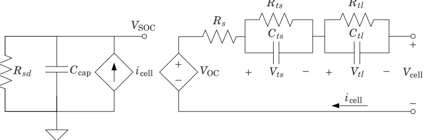
In 2006, Chen and Rincón-Mora proposed a combination of a runtime-based

model and an impedance-based model consisting of a series resistor and two parallel

resistor-capacitor networks [28]. A schematic for their model is shown in Figure 2.1.

The elements of the impedance part of the model had parameters that depended on

the SOC. Additionally, the runtime model included a resistance that modeled the

self-discharge rate. Their proposed model has the advantage of accurate prediction

of the SOC using the runtime-based portion while also modeling nonlinear transient

portion. Furthermore, the battery data can be collected using EIS measurements,

which requires neither detailed knowledge of the battery chemistry nor lengthy,

low-rate discharge experiments.

1.2.6

Evaluation

Of the model types, only some are fit for use with filtering algorithms. The

computational-intelligence and stochastic models do not adequately describe the

dynamics of the battery system for use in the filters covered by this study. On the

other hand, electrochemical, analytical, and electrical-circuit models do describe

the system dynamics in a compatible manner. Furthermore, they model the

nonlin-ear rate-capacity and recovery effects. Of these, only the electrical-circuit model has

the advantage of modeling the internal impedance of the battery, which is useful in

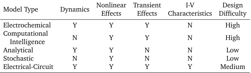
the design of battery systems. The relevant characteristics of the model types are

summarized in Table 1.1. It can be seen that electrical-circuit models are the most

suitable for this study. Among them, the proposal by Chen and Rincón-Mora is most

appropriate for the purposes of this thesis, because it is the only one discussed by

this paper that describes both the capacity and the transient effects. Therefore, their

proposed model is used for simulating the battery and comparing the performance

Table 1.1: Summary of relevant characteristics of various battery model types.

Model Type Dynamics Nonlinear Effects

Transient Effects

I-V Characteristics

Design Difficulty

Electrochemical Y Y Y N High

Computational

Intelligence N Y Y N High

Analytical Y Y N N Low

Stochastic N Y N N Low

of different filters.

1.3

Nonlinear Filtering Methods

Filtering refers to the methodology for estimating the state of a time-varying system

that is indirectly observed through noisy measurements. Specifically, the state at the

current time is estimated using the measurements from the current and previous

times. The state of a system is a group of dynamic variables that evolve through

time, and its evolution through time is governed by a dynamic system, perturbed by

process noise. The measurements are functions of the state and the measurement

noise.

Systems are classified as either linear or nonlinear. The state dynamics and

measurements of a linear system are linear functions of the state, inputs, and noises.

Particularly, the superposition principles of additivity and homogeneity are satisfied

by a linear system. Nonlinear systems do not satisfy the principle of superposition

because the functions defining the systems are not all linear, i.e. some are nonlinear.

A battery can be modeled as a nonlinear, time-varying system, with state variables

that describe such states as the SOC and the SOH. The measurements are typically

the voltage and the current. Note that the SOH was not considered by this thesis

for reasons described in Section 1.1, so this thesis assumes the battery system is

time-invariant. Additionally, only the voltage was measured since a known resistive

load was used as an input to the system in place of the current measurement. This

replacement was done because a piecewise constant discharge profile is convenient

for simulation purposes and it is more realistic to have a constant discharge load

than a constant discharge current. A state-space representation of the battery

the following chapter.

For linear systems, the optimal filtering solution with respect to the minimum

mean squared error (MMSE) is given by the least squares solution, meaning the

least squares solution equals the posterior mean. For the Gaussian case, the best

estimate is given by a linear MMSE (LMMSE) estimator, of which the Wiener filter

for wide-sense stationary signals [29] is an example. In 1960, Kalman generalized

Wiener filtering to non-stationary, discrete-time signals [30], with continuous-time

versions derived later on. Like the Wiener filter, the Kalman filter is a sequential,

LMMSE estimator. For the special case of Gaussian noise, the Kalman filter is the

MMSE estimator. Its solution procedure is as follows. Consider a linear system in

discrete time withnstates andmmeasurements defined by

xk =Fkxk−1+Bkuk+Lwk (1.4) zk =Hkxk+Mvk, (1.5)

wherex∈_Rn_,u∈

RNu, andz∈Rmare vectors of the state variables, known inputs,

and measurements, respectively; w∼ N(0, Qk),Qk∈RNw×Nw, andv∼ N(0, Rk), Rk ∈ RNv×Nv are normally distributed noise variables; F ∈ Rn×n, B ∈ Rn×Nu,

H ∈ _Rm×n_{, L ∈}

Rn×Nw, and M ∈ Rm×Nv are matrices; and a subscript k on a

variable indicates the value of that variable at timetk, wheretk =t0+kδandδis the time step. First, the Kalman filter propagates the estimates of the state variables

ˆ

xand the estimation covariancesP ∈_Rn×n _{according to}

ˆ

xk|k−1 =Fkxˆk−1|k−1+Bkuk (1.6)

where( )ˆ indicates the estimated value. Then, the estimates are updated using the measurements according to

˜

zk =zk−Hkxˆk|k−1 (1.8) Sk =HkPk|k−1Hk>+M RkM> (1.9)

Kk =Pk|k−1Hk>S −1

k (1.10)

ˆ

xk|k = ˆxk|k−1+Kk˜zk (1.11) Pk|k = (I−KkHk)Pk|k−1. (1.12)

Note that it was assumed the noises were Gaussian. Under this assumption, the

Kalman filter produces the optimal solution in the maximum likelihood (ML) and

the maximum a posterior (MAP) senses, in addition to in the MMSE sense. However,

the Gaussian assumption is unnecessary for the Kalman filter to produce the LMMSE

estimate for a general linear system.

For nonlinear systems, optimal filtering solutions are generally intractable, so

various numerical approximation methods have been developed. Chen describes

seven categories of such methods, namely Gaussian/Laplace approximation,

it-erative quadrature, multigrid method and point-mass approximation, moment

approximation, Gaussian sum approximation, deterministic sampling

approxima-tion, and Monte Carlo sampling approximation [1]. Note that only filters using

point-based numerical approximation methods were studied, as opposed to those

using density-based methods. This was done because typical battery management

systems do not have the computational power to employ costly density-based

methods, and point-based methods use the simple LMMSE update of the Kalman

approaches, respectively. Additionally, only filters using methods from the two

most popular categories of Gaussian approximation and deterministic sampling

approximation [31] were used to further limit the scope of this study.

Gaussian approximation operates by assuming the posterior distribution is

Gaussian. Then, the Taylor-series-based extended Kalman filter (EKF) [32] or the

Gaussian-describing-function-based statistically linearized filter (SLF) [33] can be

used. Li and Jilkov state that the EKF approximates the nonlinear dynamic and

measurement functions, while the SLF simplifies the nonlinear stochastic system

to a linear system so that linear filtering results are applicable [31]. Deterministic

sampling methods are special numerical methods that estimate the mean and

covariance. This category includes the unscented Kalman filter (UKF) [34] and

the cubature Kalman filter (CKF) [35]. The main advantage of the deterministic

sampling methods is they are derivative-free. The remainder of this section details

the general implementation of these filters for a discrete-time system of the form

xk =fd(xk−1,uk) +L(xk−1,uk)wk (1.13)

zk =h(xk,uk) +M(xk,uk)vk, (1.14)

where f ∈ _Rn _{and h ∈}

Rm are nonlinear vector functions, L ∈ Rn×Nw and M ∈

Rm×Nv are nonlinear matrix functions, and the inputu is assumed to be piecewise

constant, meaning u(t) = u(tk) = uk fortk−1 < t ≤ tk. An implicit, first-order Taylor-Heun numerical integration method was used to discretize the

continuous-time dynamicsf of the chosen battery model. In particular, an iterated integration

procedure was used, as was done by Särkkä [36]. For the iterations, a superscript

of (i) indicates the ith step of a M-step iterative integration scheme. Note that ˆ

x(0)_k−1 = ˆxk−1 and xˆ (M)

notation used are discussed in Section 2.2.

1.3.1

Extended Kalman Filter

One of the most popular nonlinear filters is the extended Kalman filter (EKF), which

approximates the nonlinear state and measurement functions using Taylor series

expansion. This study uses the first-order expansion for the EKF. The prediction

step follows the discretization approach proposed by Mazzoni [37] to numerically

approximate the time dynamics in Equation (2.35) and the

continuous-time estimate covariance differential equation

˙

P =F(x,u)P +P F>(x,u) +L(x,u)QL>(x,u), (1.15)

with the JacobianF =∂f/∂x. The discretizationfdoff is given in Section 2.2, and the discretion of the estimate covariance matrix is as follows. Note that an M-step

iterative integration method was used for the discretization off. Thus, a similar

iterative procedure was used for the discretion of the estimate covariance matrix.

For a time step ofδ= (tk−tk−1)/M, whereM is a positive integer, the prediction step consists ofM iterations of the following equations:

ˆ

x(_ki₋)_1|k−1 =fd(ˆx (i−1)

k−1 ,uk, δ, i) (1.16)

P_k(₋i)_1|k−1 = P_k(i₋−₁1)_|k−1 +Gτ n

F(ˆxτ,uk)P (i−1)

k−1|k−1+P (i−1) k−1|k−1F

>_(ˆx τ,uk) +L(ˆxτ,uk)QτL>(ˆxτ,uk)

o G>_τδ,

(1.17)

wheretτ =tk−1+δ(i+ 1/2),

Gτ =

I−F(ˆxτ,uk) δ 2

−1

and

ˆ

xτ = 1 2

ˆ

x(_ki₋−₁1)+ ˆx(_ki₋)₁−F(ˆx(_ki₋)₁,uk)f(ˆx (i) k−1)

δ2 4

. (1.19)

The iteration given by Equations (1.16) and (1.17) is repeatedM-times to complete

the prediction step. It can be seen that the differential equation for the covariance

matrix was approximated using a modified Gauss-Legendre formula with an implicit

increment rule, following Mazzoni. The numerical approximations for the state

and covariance are both A-stable, which is necessary for the chosen battery model,

and consistent to the first-order. The update equations for the EKF come from the

LMMSE filter and are

Kk =Pk|k−1Hk> HkPk|k−1Hk>+M(ˆxk)RkM>(ˆxk) −1

(1.20)

ˆ

xk|k = ˆxk|k−1+Kk zk−h(ˆxk|k−1)

(1.21)

Pk|k = (I−KkHk)Pk|k−1, (1.22)

with the JacobianH =∂h/∂x.

1.3.2

Unscented Kalman Filter

The unscented Kalman filter (UKF) is an efficient, generally derivative-free filtering

algorithm that relies on the unscented transformation (UT). The UT is useful for

forming the Gaussian approximation to the joint distribution of random variables

x andy forx ∼ N(m, P)andy =g(x), wherex ∈_Rn_{,y ∈}

Rm, andg :Rn 7→ Rm is a nonlinear function. Then, the first and second moments corresponding to

approximation of the joint probability density ofxandy has the form    x y   =N

      m µU   ,   

P CU

C_U> SU 

 





. (1.23)

Then, the UT picks2n+ 1 sample points{xi}, commonly known as sigma points, along with the same number of weights {wi}, as follows [38]. First, the sigma

points are chosen from the columns of the matrixp(n+λ)P, giving

x(0)=mx (1.24)

x(i)=mx+ hp

(n+λ)Pi

i, i= 1, . . . , n (1.25) x(i)=mx−

hp

(n+λ)Pi i−n

, i=n+ 1, . . . ,2n (1.26)

with the weights

W₀(m)= λ

n+λ (1.27)

W₀(c)= λ

n+λ + (1−α

2_{+β) (1.28)}

W_i(m)=W_i(c) = 1

2(n+λ), i= 1, . . . ,2n. (1.29)

The parameterλis defined as

λ =α2(n+κ)−n, (1.30)

and the constantsα,β, and κare parameters of the method. For the UKF,α is a

typically0. Each sigma point is transformed by

y(i) =g(x(i)), i= 0, . . . ,2n. (1.31)

Then, the moments are approximated by

µU = 2n X

i=0

W_i(m)y(i) (1.32)

SU = 2n X

i=0

W_i(c)(y(i)−µU)(y(i)−µU)> (1.33)

CU = 2n X

i=0

W_i(c)(x(i)−m)(y(i)−µU)>. (1.34)

The square root of the positive definite matrix P is defined as a matrix A such

that P =AA>. Note thatAis not unique. For performance reasons, the Cholesky factorization is typically used.

Let the described UT algorithm be denoted by

[µU, SU, CU] = UT(g, m, P). (1.35)

Then, for the discretized system in Equations (1.13) and (1.14), for an M-step

numerical integration scheme, the prediction step for the UKF can be written as

[ˆx(_ki₋)_1|k−1,P˜_k(₋i)_1|k−1] = UT(fd,xˆ(i −1) k−1|k−1, P

(i−1)

k−1|k−1) (1.36) P_k(i₋)_1|k−1 = ˜P_k(₋i)_1|k−1+L(ˆx(_ki₋)_1|k−1)QkL>(ˆx

(i)

k−1|k−1), (1.37) (1.38)

by

[µk,S˜k, Ck] = UT(h,xˆk|k−1, Pk|k−1) (1.39) Sk = ˜Sk+M(ˆxk|k−1)RkM>(ˆxk|k−1) (1.40)

Kk =CkS_k−1 (1.41)

ˆ

xk|k = ˆxk|k−1+Kk(zk−µk) (1.42) Pk|k =Pk|k−1−KkSkKk>. (1.43)

Note that the mean and covariances were estimated using the UT, and the update

is equivalent to the LMSSE update used in the Kalman filter.

For numerical stability reasons, this study employed a change to the above UKF

procedure as suggested by Julier et al. [39]. In Equation (1.36), the covariance is

estimated by

˜

Pk|k−1 = 2n X

i=0

W_i(c)(ˆx_k(i_|)_k−1−xˆ(0)_k|k−1)(ˆx(_ki_|)_k−1−xˆ(0)_k|k−1)>, (1.44)

where the covariance is evaluated about the projected mean rather than the

weighted mean. This change ensures the positive definiteness of the covariance

matrix, as required by the definition of covariance. Another change, discovered by

the author, that results in better numerical stability and lower MSE is the estimation

of the cross-covariance in Equation (1.39) by

Ck= 2n X

i=0

W_i(c)( ˆχ(_ki_|)_k−1−χˆ(0)_k|k−1)(ˆz_k(i)−µk)>, (1.45)

mean xˆ(0)_k|k−1 and the weighted mean µk. The increase in stability and accuracy with the change in Equation (1.45) was discovered through experimentation. The

reason for the improvement is unknown, but the change was used to produce the

simulation results.

1.3.3

Cubature Kalman Filter

The cubature Kalman filter (CKF) is similar to the UKF except that it uses the

spherical-radial cubature rule rather than the UT to approximate the Gaussian

inte-grals. Indeed, the prediction and update steps of the CKF follow Equations (1.36)

to (1.43) except that the UT algorithms in Equations (1.36) and (1.39) are replaced

by the corresponding cubature algorithm. This thesis explores the third-order

and fifth-order CKFs, whose implementations are discussed in the following two

sections.

1.3.3.1 Third-Order CKF

The third-order spherical-radial CKF of Arasaratnam et al. [35, 40] is a special case

of the UKF withα= 1,β = 0, andκ= 0. The third-order cubature rule chooses2n cubature points, giving [35]

x(i)=mx+ h√

nPi

i, i= 1, . . . , n (1.46) x(i)=mx−

h√ nPi

i−n

where the matrix square root is computed using Cholesky factorization, as in the

UT. Then, the moments are approximated by

µU = 1 2n

2n X

i=1

y(i) (1.48)

SU = 1 2n

2n X

i=1

(y(i)−µU)(y(i)−µU)> (1.49)

CU = 1 2n

2n X

i=1

(x(i)−m)(y(i)−µU)>. (1.50)

The prediction and update steps follow Equations (1.36) to (1.43) with the UTs

in Equations (1.36) and (1.39) replaced by the third-order cubature rule given by

Equations (1.46) to (1.50). The resulting third-order CKF is exact for polynomials

of order three. Compared to the UKF, the third-order CKF is numerically more stable

due to its positive weights. While the UKF has some desirable theoretical properties,

its weights can be negative, causing numerical problems in some cases [36].

To increase numerical stability and accuracy, a change similar to that in

Equa-tion (1.45) was used, giving

Ck = 1 2n

2n X

i=0

( ˆχ(_ki_|)_k−1−xˆk|k−1)(ˆz (i)

k −µk)>, (1.51)

where χˆ(_ki_|)_k−1 are the cubature points whose average isxˆk|k−1. This change was verified through experimentation to produce better results.

1.3.3.2 Fifth-Order CKF

The fifth-order spherical-radial CKF is a higher-order extension of the third-order

cubature points, giving [41, 42]

x(0) =mx (1.52)

x(i)=mx+ h√

n+ 2ei i

, i= 1, . . . , n (1.53)

x(i)=mx− h√

n+ 2ei−n i

, i=n+ 1, . . . ,2n (1.54)

x(i)=mx+ h√

n+ 2s+_i−2ni, i= 2n+ 1, . . . ,2n+ n(n−1)

2 (1.55)

x(i)=mx− h√

n+ 2s+_{i−2n−n(n−1)/2}i, i= 2n+ n(n−1)

2 + 1, . . . ,2n+n(n−1) (1.56)

x(i)=mx+ h√

n+ 2s−_{i−2n−n(n−1)}i, i= 2n+n(n−1) + 1, . . . ,2n+ 3n(n−1) 2 (1.57)

x(i)=mx− h√

n+ 2s−_{i−2n−3n(n−1)/2} i

, i= 2n+ 3n(n−1)

2 + 1, . . . ,2n 2

, (1.58)

whereei are the columns of the Cholesky factorization √

P and

s±_i =

1

√

2(ej±ek) :j < k;j, k = 1,2, . . . , n

(1.59)

are scaled linear combinations of the columns ei. The weights on the points are

W0 = 2

n+ 2 (1.60)

Wi =

4−n

2(n+ 2)2, i= 1, . . . ,2n (1.61) Wi =

1

(n+ 2)2, i= 2n+ 1, . . . ,2n

Then, moments are approximated by

µU = 2n2 X

i=0

Wiy(i) (1.63)

SU = 2n2 X

i=0

Wi(y(i)−µU)(y(i)−µU)> (1.64)

CU = 2n2 X

i=0

Wi(x(i)−m)(y(i)−µU)>. (1.65)

As in the third-order CKF, the prediction and update steps follow Equations (1.36)

to (1.43) with the UTs in Equations (1.36) and (1.39) replaced by the fifth-order

cubature rule given by Equations (1.53) to (1.65). Note that unlike the third-order

CKF and like the UKF, the weights of the fifth-order CKF can be negative.

As in the third-order CKF, to increase numerical stability and accuracy, a change

similar to that in Equation (1.45) was used, giving

Ck = 2n2 X

i=0 Wi(ˆx

(i)

k|k−1−ˆxk|k−1)(ˆz (i)

k −µk)>. (1.66)

whereχˆ(_ki_|)_k−1are the cubature points whose weighted average isxˆk|k−1. This change was verified through experimentation to produce better results.

1.3.4

Statistically Linearized Filter

In the statistically linearized filter (SLF), the nonlinear state and measurement

functions are statistically linearized to minimize the MSE. Then, the resulting

x∼ N(m, P), the nonlinear functionf(x)is linearized as [31, 33, 43]

f(x)≈b+A(x−m), (1.67)

where the parametersbandAare chosen to minimize the error

MSE(b, A) =Ekf(x)−b−A(x−m)k2

. (1.68)

Differentiating the MSE expression and setting the derivatives to zero, produces

the optimal values

b=E[f(x)] (1.69)

A=E[f(x)(x−m)>]P−1. (1.70)

These values reproduce the mean exactly but the covariance is an approximation.

The expectations can be calculated analytically or numerically. Due to the

dif-ficulty of finding the analytical forms of the expectations, this study chooses to

approximated them numerically using the third-order spherical-radial cubature

rule described in Section 1.3.3.1, which has the advantages of numerical stability

and low computational complexity compared to the UT and fifth-order cubature

rule, respectively. The cubature approximation results in

bx=E[fd(x)]≈ 1 2n

2n X

i=1

fd(x(i)) (1.71)

Ax=E[f(x)(x−m)>]E[(x−m)(x−m)>]−1 =E[F(x)]≈

1 2n

2n X

i=1

for the expectations of the state mean and covariance and

bz=E[h(x)]≈

1 2n

2n X

i=1

h(x(i)) (1.73)

Az=E[h(x)(x−m)>]E[(x−m)(x−m)>]−1 =E[H(x)]≈

1 2n

2n X

i=1

H(x(i))

(1.74)

for the expectations of the measurement state and covariance, where the cubature

points come from the columns of √nP. With the given statistically optimal

lin-earization, the resulting linear system can be filtered using a procedure similar to

the linear Kalman filter. The prediction phase, for anM-step numerical integration

scheme, consists of peforming the following equationsM times fori= 1, . . . , M using the notation from Section 2.2:

ˆ

x(_ki₋)_1|k−1 =b_ˆx(i−1) k−1|k−1

(1.75)

P_k(₋i)_1|k−1 =A_ˆx(i−1) k−1|k−1

P_k(i₋−₁1)_|k−1A> ˆ

x(_k−i−₁1)_|k−1 +L(ˆx (i−1)

k−1|k−1,u)QkL >

(ˆx(_ki₋−₁1)_|k−1,u), (1.76)

where the above equations are iterated overi = 1, . . . , M. Note that the form is very similar to the Kalman filter prediction steps given by Equations (1.6) and (1.7),

whereE[x−m] = 0has been used to simplify the calculation forxˆk|k−1. The update phase consists of

Sk =AzPk|k−1A>z +M(x,u)RkM>(x,u) (1.77)

Kk =Pk|k−1A>zS

−1

k (1.78)

ˆ

xk|k = ˆxk|k−1+Kk(zk−bz) (1.79)

Again, this is very similar to the Kalman filter update steps given by Equations (1.8)

to (1.12). The SLF is similar to the EKF in the sense that its equations have a similar

form to the Kalman filter equations. In fact, ignoring the numerical approximation

of the expectations, the SLF uses first-order Fourier-Hermite series expansion to

approximate the nonlinear functions whereas the EKF uses Taylor series expansion.

Furthermore, the SLF implementation of this study uses the same mean estimation

method as the third-order CKF. The covariance estimation differs because the SLF

Chapter

2

Problem Setup

2.1

Battery Model

As discussed in the previous section, this thesis considers the electrical-circuit

battery model proposed by Chen and Rincón-Mora [28] shown in Figure 2.1. The

left portion of the circuit models the capacity, SOC, and runtime, while the right

portion models the transient I-V characteristics. For convenience, the model is

designed so that the SOC of the battery equals the voltage VSOC, in volts. The

parametersCcapandRsd are assumed constant for a given battery and determine

i_cell

i_{cell + +}

+

+

− −

− −

Rsd

V_SOC

C_cap V_OC V_cell

Rs

Rts

Cts

Vts

Rtl

Ctl

Vtl

the capacity and self-discharge rate of the battery. The other parameters are all

nonlinear functions of VSOC and determine the transient I-V response as well as

the open-circuit voltageVOC. From a typical TCL PL-383562 polymer lithium-ion

battery, Chen and Rincón-Mora extracted these parameters experimentally and fit

them to curves, obtaining

Rs(VSOC) = 0.1562e−24.37VSOC + 0.07446 (2.1)

Rts(VSOC) = 0.3208e−29.14VSOC+ 0.04669 (2.2)

Cts(VSOC) =−752.9e−13.51VSOC + 703.6 (2.3)

Rtl(VSOC) = 6.603e−155.2VSOC + 0.04984 (2.4)

Ctl(VSOC) =−6056e−27.12VSOC+ 4475 (2.5)

VOC(VSOC) =−1.031e−35VSOC + 3.685 + 0.2156VSOC−0.1178VSOC2 + 0.3201VSOC3

(2.6)

The resistance and capacitance parameters shown above are approximately constant

for SOC >0.2and change exponentially for SOC<0.2. The open-circuit voltage also changes exponentially for SOC <0.2but is approximately linear for SOC>0.2. Note that the capacitances Cts andCtl are negative for SOC values close to zero,

which is both unrealistic according to the experimental data collected by Chen and

Rinón-Mora and mathematically problematic. To solve this, a lower bound was

placed on theV_SOCinput to the capacitance functions. Thus, for inputs below some

producing

ˆ

Cts(VSOC) =

   

  

Cts(VSOC), VSOC≥vT

Cts(vT), VSOC< vT

(2.7)

ˆ

Ctl(VSOC) =

   

  

Ctl(VSOC), VSOC≥vT

Ctl(vT), VSOC< vT

(2.8)

The thresholdvT was chosen based on the experimental data of Chen and

Rinón-Mora, specifically so that the threshold capacitance values are approximately

equal to the lowest such values measured by them. A threshold of vT = 0.015 V accomplishes this goal.

This study used the nonlinear parameters given by Chen and Rincón-Mora for

the implementation of a battery using their battery model in Matlab. In addition,

the thresholding defined in Equations (2.7) and (2.8) was used with vT = 0.015 V. The other, constant parameters were chosen to produce a capacity of1 Ahand a self-discharge rate of4% per month. To do so, the capacitanceCcap was calculated

to hold the desired capacity whenVSOC = 1 V, and then the resistanceRsd was set to produce the desired self-discharge rate. For a given capacity ofC† in Ah,Ccapis

Ccap =

Q V_SOC =

C†

1V = 3600C

†_{[F]. (2.9)}

Next, the resistanceRsd is chosen so that the time constantτ =RC results in the desired drop ofξ = 0.04overT = 1 month as follows

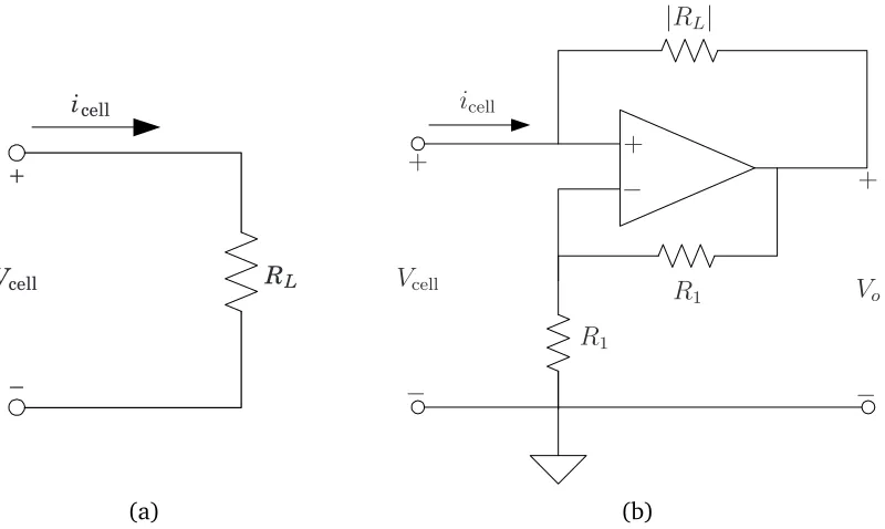
Then,Rsd =τ /Ccap. Thus, the parameters areCcap = 3600 FandRsd = 17.6376 kΩ. In order to simulate the use of the modeled battery, discharging and charging

loads were implemented, as shown in Figures 2.2. For discharging, a resistive load

RLis placed across the battery terminals, creating a discharge rate oficell =Vcell/RL. For charging, a negative resistance−RL, whereRL>0, is used, creating a charging current of −icell = Vcell/RL. Thus, any arbitrary charging or discharging current can be set by choosing the appropriate resistanceRL. Furthermore, an open circuit

can be simulated by choosing RL sufficiently large so that icell ≈ 0. Additional

consideration has to be taken to ensure that the constant current and constant

voltage charging conditions in standard charging procedure can be produced using a

negative resistance. Typically, the specific battery modeled by the given parameters

is charged at a rate of C5/5 until a terminal voltage of 4.2 V is reached, where C5/5is the discharge rate at which a full battery is completely discharged in five

hours [44]. Then, the battery is charged at a constant voltage of 4.2 V until the

icell

Vcell

+

−

RL

(a)

icell

Vcell _V

o

+ +

+

− −

−

|RL|

R1

R1

(b)

charging current is below C5/20. The constant current condition can be met by

varyingRLso thatVcell/RL stays constant, while the constant voltage condition is

met by varyingRL so thaticellRLstays constant.

This use of the loadRLto control the current icell means it is the input to the

system. Moreover, the measurable outputs of the system are Vcellandicell. However,

since knowledge of one of them along with RL allows for the calculation of the

other, the two outputs have a known relationship between them. Therefore, only

one of the outputs is necessary to fully define the input-output relationship of the

system. In this study, the voltage Vcell was chosen as the measured output as is

typical for single-measurement battery system models.

For ease of numerical simulation, it is useful to find the state-space system for

the circuit. The state-space representation is derived using the physical variable

definition, in which the state variables are chosen to represent the voltages across

the capacitors. Choosingx1 =VSOC,x2 =Vts, andx3 =Vtl achieves this goal and results in the state-space representation

˙ x1 =−

x1 RsdCcap

− VOC(x1)−x2 −x3

(Rs(x1) +RL)Ccap

+fw,1(x, RL,w) (2.12)

˙ x2 =−

x2 Rts(x1)Cts(x1)

+ VOC(x1)−x2−x3 (Rs(x1) +RL)Cts(x1)

+fw,2(x, RL,w) (2.13)

˙ x3 =−

x3 Rtl(x1)Ctl(x1)

+ VOC(x1)−x2−x3 (Rs(x1) +RL)Ctl(x1)

+fw,3(x, RL,w) (2.14)

Vcell =

VOC(x1)−x2−x3 1 +Rs(x1)/RL

+fv(x, RL,v), (2.15)

where RL is the input to the system, Vcell is the output, fw is the process noise

function, fv is the measurement noise function, and the nonlinear parameters

depending onx1 are given by Equations (2.1) to (2.6) along with the thresholding

system is nonlinear to both the input and the states. In order to establish the noise

expressions, the types of noise present in the battery have to first be determined.

This thesis assumed that the process and measurement noises in this system are

due to thermal noise in the resistances for the internal impedance of the battery

Rs,Rts, andRtl, and for the loadRL. This was motivated by measurements of the

voltage noise in batteries conducted by Boggs et al. that showed the measured noise

is mainly due to thermal noise since shot noise is suppressed by the correlation

between the battery terminals [45]. This thermal noise was assumed to be Gaussian

white noise with a power spectral density (PSD) of [46]

Sn(ω)∼= 2kT watts per Hz for |ω| 2πkT /h, (2.16)

where T is the temperature of the conducting medium in Kelvin, k is the

Boltz-mann’s constant, and his the Planck’s constant. Figure 2.3 shows that the thermal

noise due to the resistances modeled as voltage sources in series with the

resis-tances, with PSDs of Sv(ω) = 2kT Rfor a corresponding resistance R. Using this definition, the noise functions are given by

i_cell

+

+

+

+

+

+

+

+

−

−

−

−

−

−

− −

VOC _Vcell

Rs

Rts

Cts

Vts

Rtl

Ctl

Vtl

RL vns

vn_ts vn_tl

vn_L

fw,1 =

vns +vnL (Rs(x1) +RL)Ccap

(2.17)

fw,2 =

vnts Rts(x1)Cts(x1)

− vns +vnL (Rs(x1) +RL)Cts(x1)

(2.18)

fw,3 =

vntl Rtl(x1)Ctl(x1)

− vns +vnL (Rs(x1) +RL)Ctl(x1)

(2.19)

fv =−

vns +vnL 1 +Rs(x1)/RL

. (2.20)

It can be seen that the resistances change over time, which causes the PSD of the

sourcesvnto also change. For the purposes of modeling, it is useful to define noise

variables that have constant PSDs. Using the square root of the power supplied

by the noise sources as the noise variables accomplishes this goal and produces

the variablesw1 =vns/

√

Rs,w2 =vnts/

√

Rts,w3 =vntl/

√

Rtl, andw4 =vnL/ p

|RL|

along with v1 = vns/

√

Rs and v2 = vnL/ p

|RL|, which all have constant PSDs of

2kT. Note the use of the absolute value ofRLin the definition of w4 and v2, since RLcan become negative. In the case of RL< 0, their PSDs remain at2kT while the sign ofvnL is negated, which is implemented in the system using the signum

function, defined as

sgn(x) :=               

−1 ifx <0

0 ifx= 0

1 ifx >0.

(2.21)

Then, the state space representation of the system becomes

˙ x1 =−

x1 RsdCcap

−VOC(x1)−x2−x3− p

Rs(x1)w1 −sgn(RL) p

|RL|w4 (Rs(x1) +RL)Ccap

(2.22)

˙ x2 =−

x2− p

Rts(x1)w2 Rts(x1)Cts(x1)

+VOC(x1)−x2−x3− p

Rs(x1)w1−sgn(RL) √

RLw4 (Rs(x1) +RL)Cts(x1)

˙ x3 =−

x3− p

Rtl(x1)w3 Rtl(x1)Ctl(x1)

+VOC(x1)−x2−x3− p

Rs(x1)w1−sgn(RL) √

RLw4 (Rs(x1) +RL)Ctl(x1)

(2.24)

Vcell =

VOC(x1)−x2−x3− p

Rs(x1)v1−sgn(RL) √

RLv2 1 +Rs(x1)/RL

. (2.25)

It can be seen that the system can be written in the form

˙

x(t) = f(x(t),u(t),pQw(t)) (2.26)

z(t) = h(x(t),u(t),√Rv(t)), (2.27)

wherexis the state,uis the input,f is the nonlinear differential equation for the

state, h is the nonlinear measurement function, andwand vare scaled Wiener

processes used to represent the integral of the Gaussian white-noise noise sources.

Specifically, the Wiener processes were scaled by the square roots ofQ= 2kT I4 and R = 2kT I2, where their diagonals are the values of the PSDs of the noise sources and In is then-dimensional identity matrix. It is useful to find the derivatives of

f andh with respect to x, w, and v for use with the filters. This thesis defines

Their equations are F =                                   −1

R_sdCcap +

(V oc−x2−x3)R0s −(Rs+RL)VOC0 (R_s+R_L)2_C

cap

(RtsCts)0x2

RtsCts

+

(R_s+R_L)C_tsV0

OC

−(V oc−x2−x3)

(Rs+RL)Cts 0

(Rs+RL)Cts 2

(RtlCtl)0x3

RtlCtl

+

(Rs+RL)CtlVOC0

−(V oc−x2−x3)

(Rs+RL)Ctl 0

(Rs+RL)Ctl 2

. . . 1

(Rs+RL)Ccap

1 (Rs+RL)Ccap

. . . −1 RtsCts

+ −1

(Rs+RL)Cts

−1 (Rs+RL)Cts

. . . −1

(Rs+RL)Ctl

−1

RtlCtl

+ −1

(Rs+RL)Ctl                                   (2.28) H =  

(1 +Rs/RL)VOC0

−(VOC−x2−x3)Rs0/RL (1 +Rs/RL)2

−1 1 +Rs/RL

−1 1 +Rs/RL

  (2.29) L=             √ Rs (Rs+RL)Ccap

0 0 sgnRL

p |RL| (Rs+RL)Ccap

−√Rs (Rs+RL)Ccap

√

Rts RtsCts

0 −sgnRL p

|RL| (Rs+RL)Ccap

−√Rs (Rs+RL)Ccap

0

√

Rtl RtlCtl

−sgnRL p

|RL| (Rs+RL)Ccap

            (2.30) M =

−√Rs 1 +Rs/RL

−sgnRL p

|RL| 1 +Rs/RL

, (2.31)

off with respect tox. Due to symmetry and∂2_f

k/∂xi∂xj = 0fori, j = 2,3, only the first column of each tensor component of the Hessian is given. The resultant

Hessian is

∂2f1 ∂xi∂x1

=              

(Rs+RL)

(VOC−x2−x3)Rs00−(Rs+RL)VOC00

−2R0_s(VOC−x2−x3)R0s−(Rs+RL)V_OC0

(Rs+RL)3Ccap

−R0_s (Rs+RL)2Ccap

−R0_s (Rs+RL)2Ccap

              (2.32)

∂2f2 ∂xi∂x1

=                

RtsCts(RtsCts)00

−

(RtsCts)02

x2

(RtsCts)2 +

(Rs+RL)Cts

(Rs+RL)CtsV00

OC−(VOC−x2−x3)

(Rs+RL)Cts00 + 2

(Rs+RL)Cts0

(Rs+RL)CtsVOC0 −(V oc−x2−x3)

(Rs+RL)Cts0

(Rs+RL)Cts3

(RtsCts)0

RtsCts +

(Rs+RL)Cts0

(Rs+RL)Cts2

(Rs+RL)Cts0

(Rs+RL)Cts2

                (2.33)

∂2_f 3 ∂xi∂x1

=                

RtlCtl(RtlCtl)00

−

(RtlCtl)02

x3

(RtlCtl)2 +

(Rs+RL)Ctl

(Rs+RL)CtlVOC00 −(VOC−x2−x3)

(Rs+RL)Ctl00 + 2

(Rs+RL)Ctl0

(Rs+RL)CtlV0

OC−(V oc−x2−x3)

(Rs+RL)Ctl0

(Rs+RL)Ctl3

(Rs+RL)Ctl0

(Rs+RL)Ctl2

(RtlCtl)0

RtlCtl +

(Rs+RL)Ctl0

(Rs+RL)Ctl2

                (2.34)

Moreover, based on the forms of the JacobiansLandM, the battery system can be

written as

˙

zk =h(xk,uk) +M(xk,uk) √

Rv(tk)δ, (2.36)

where Q and R are defined the same as in Equations (2.26) and (2.27), In is

the n × n identity matrix, and δ = tk −tk−1 is the time step for the discrete-time measurements. Note that the state dynamics are in continuous-discrete-time. The

discretization of the continuous-time dynamics for use with the filters is discussed

in the next section. Additionally, for convenience, the quantity√Rv(tk)δ will be referred to as vk. Note thatvk ∼ N(0, δR)is a Gaussian random variable whose covariance is the PSD of the measurement noise sources scaled by the time step.

2.2

Discretization of System Dynamics

In the prediction phases of the filters, the expected value of the continuous-time

differential equation for the state in Equation (2.35) needs to be computed. In

order to find the state x(tk)from the statex(tk−1), assuming the input is constant, the equation can be solved numerically. Assume that the discretized system has the

form

˙

xk=fd(xk−1,uk) +L(xk−1,uk) p

Qw(tk)δ. (2.37)

For convenience, let wk = √

Qw(tk)δ, where δ =tk−tk−1 is the time step. Note thatwk ∼ N(0, δQ)is a Gaussian random variable whose covariance is the PSD of the process noise sources scaled by the time step. Additionally, recall thatvkis also

a Gaussian random variable. Then, the discrete-time system is given by

˙

wherewk∼ N(0,2kT δI4)andvk ∼ N(0,2kT δI2). The scaling of the covariances byδ is from the conversion of the continuous-time Wiener processes to the

discrete-time Gaussian random variables.

Särkkä and Solin state that a linearized discretization approach, in which the

continuous-time system is first discretized and then approximated as Gaussian,

tends to work better than a discretized linearization approach, in which the system

is first approximated as a Gaussian process and then discretized [36]. This thesis

follows this guideline and performs the prediction using linearized approximations

of a discretization of the continuous-time dynamics. To increase the accuracy of

the discretized integration in the prediction phase, the sampling period is divided

into M steps of equal length and the integration is performed in M steps. The

motivation for this iterated integration comes from the definition of order for an

Itô-Taylor expansion of a stochastic differential equation. An expansion is said to

be strongly convergent with orderβ if for any positive integerM and time interval

[tk−1, tk], the error of theM-step approximation satisfies [47]

E "

sup t∈[tk−1,tk]

|x(t)−xˆ(M)(t) #

≤λ(δ(M))β, (2.40)

wherex(t)is exact solution,x(M)(t)is theM-step approximation,δ = (tk−tk−1)/M andλis a constant uniform inM. It can be seen that the error of the approximation

decreases as the number of integration steps M increases.

Furthermore, note that the system is extremely stiff based the definition of the

stiffness ratio as the ratio of the largest eigenvalue ofF to its smallest eigenvalue,

whereF is the Jacobian of the dynamics f(x,u); when the stiffness ratio is much greater than unity, the system is stiff [48, 49]. From EIS studies of batteries, the

transport effects like diffusion are on the order of10−6 _to100 _{Hz, middle frequency} effects caused by charge transfer and the electrochemical double layer are on the

order of 100 _{to 10}3 _{Hz, and the high frequency conductance and skin effects are} on the order of 103 _{to 10}4 _{Hz [50]. Therefore, the approximate stiffness ratio} is 1010 _{1, and the system is stiff. As a result of the stiffness, any numerical} integration method needs to be A-stable, i.e. the method converges for all systems

whose eigenvalues have negative real parts. For example, simulation results show

that the fourth-order Runge-Kutta method diverges even at step sizes < 10−2 seconds.

This thesis uses the linearized discretization approach proposed by Mazzoni,

in which the differential equation is first discretized and then approximated using

Taylor series expansion [37]. This approach has the advantage of A-stability. The

discretization is performed using the trapezoidal approximation (Heun’s method)

of Equation (2.35), where E[wk] = 0 is used so that only the integration of f needs to be considered. For convenience, denote the value of a quantity at time

tk using the subscriptk and assume thatδ=tk−tk−1 is the time step. Then, the approximation produces

xk ≈xk−1+ 1

2 f(xk−1,uk) +f(xk,uk)

δ. (2.41)

The vector field f at xk is approximated by first-order Taylor expansion around

xk−1, giving

xk ≈xk−1+f(xk−1,uk)δ+ 1