Application of WASPAS Method as an Optimization Tool in Non-traditional Machining Processes

Application of WASPAS Method as an Optimization Tool in Non-traditional

Machining Processes

Shankar Chakraborty

_{, Orchi Bhattacharyya}

_,

Edmundas Kazimieras Zavadskas

_{, Jurgita Antucheviciene}

1_{Department of Production Engineering, Jadavpur University,}

Kolkata - 700 032, West Bengal, India

e-mail: [email protected], [email protected]

2_{Department of Construction Technology and Management, Vilnius Gediminas Technical University,}

Sauletekio al.11, LT-10223 Vilnius, Lithuania

e-mail: [email protected], [email protected]

http://dx.doi.org/10.5755/j01.itc.44.1.7124

Abstract. In order to meet the present day manufacturing requirements of high dimensional accuracy and generation of intricate shapes in difficult-to-machine materials, non-traditional machining (NTM) processes are now becoming the viable options. The product features that cannot be machined using the conventional material removal processes can now be easily generated employing the NTM processes due to their various added advantages. To achieve enhanced machining performance of the NTM processes, it is always desirable to determine the optimal settings of various control parameters of those processes. It has been observed that the optimal parametric combinations attained applying different optimization techniques may not usually belong amongst the conducted experimental trials and the process engineer may have to perform additional experiments to achieve the desired machining goals. In this paper, the applicability of weighted aggregated sum product assessment (WASPAS) method is explored for parametric optimization of five NTM processes. It is concluded that WASPAS method can be deployed as an effective tool for both single response and multi-response optimization of the NTM processes. It is also observed that this method is quite robust with respect to the changing coefficient (λ) values.

Keywords: WASPAS method; Optimization; Process parameter; Response.

1. Introduction

Non-traditional machining (NTM) processes are those metal removal processes mainly applied to fulfill the present day requirements of aerospace, nuclear, missile, turbine, automobile, tool and die-making industries. Metal removal processes (conventional and non-conventional) are those machining operations by which undesired material is removed from the work-piece to generate a required shape feature on it. The NTM processes are now being successfully employed for machining of newer and harder materials with higher strength, hardness, toughness and other diverse mechanical properties. Many of the materials, like titanium, stainless steel, high-strength-temperature-resistant alloys, fiber-reinforced composites, ceramics and refractories, which cannot be machined by the conventional material removal processes, are now being machined using the NTM processes. These

*_{corresponding author}

processes is becoming increasingly unavoidable and popular at the shop floor, especially when there is a demand for micro- and nano-machining operations in the present day manufacturing environment. Thus, for effective utilization of the capabilities of different NTM processes, an in-depth knowledge about various machining characteristics of those processes is of utmost importance [1-3].

Each of the NTM processes has several control parameters (process parameters) which significantly influence the responses or outputs of those processes. Achievement of the maximum machining performance of the NTM processes thus depends on the optimal settings of those process parameters. Several mathema-tical tools and techniques, like Taguchi method [4], steepest ascend method, desirability function approach [5], artificial neural network and numerous advanced optimization methods have already been applied by the past researchers for parametric optimization of the NTM processes. The main problem of the previously adopted techniques lies in the fact that the optimal parametric settings did not sometimes belong amongst the conducted experimental trials and the process engineers might have to perform additional experi-ments in order to optimize the considered responses. Sometimes, the derived optimal parametric combina-tions may not be available among the present settings of the given NTM setup. To avoid this shortcoming, in this paper, the application of weighted aggregated sum product assessment (WASPAS) method is proposed for parametric optimization of five popular NTM pro-cesses. Its capability as a single response and multi-response optimization tool is also validated.

2. WASPAS method

The WASPAS method is a unique combination of two well-known multi-criteria decision-making (MCDM) approaches, i.e. weighted sum model (WSM) and weighted product model (WPM). Its application first requires development of a decision matrix, X = [xij]m×n where xij is the performance of the ith alternative

with respect to the jth _{criterion, m is the number of}

candidate alternatives and n is the number of evaluation criteria. To have the performance measures comparable and dimensionless, all the entries of the decision matrix are linear normalized using the following two equations: ij i ij ij x x x max

 for beneficial criteria, (1)

i.e. if max

𝑖 𝑥𝑖𝑗 value is preferable and

ij ij i ij x x

x min for non-beneficial criteria, (2)

if min

𝑖 𝑥𝑖𝑗 value is preferable and xijis the normalized

value of xij.

In WASPAS method, a joint criterion of optimality is sought based on two criteria of optimality. The first criterion of optimality, i.e. criterion of a mean weighted success is similar to WSM method. It is a popular and well accepted MCDM approach applied for evaluating a number of alternatives with respect to a number of decision criteria. Based on WSM method [6-7], the total relative importance of the ith _{alternative is}

calculated as follows:





i

x

w

Q

, (3)

where wj is weight (relative importance or significance)

of the jth _{criterion. The weight of a particular criterion}

can be determined using analytic hierarchy process or entropy method [8].

On the other hand, according to WPM method [7, 9], the total relative importance of the ith _{alternative is}

evaluated using the following expression:



( . (4)

A joint generalized criterion of weighted aggregation of additive and multiplicative methods is then proposed as follows [10]:

   













x

w

x

Q

Q

Q

.

)

(

5

.

0

5

.

0

5

.

0

5

.

0

In order to have increased ranking accuracy and effectiveness of the decision-making process, in WASPAS method, a more generalized equation for determining the total relative importance of the ith

alternative is developed [11] and further applied [12-13] as below:

 

_

_





_

















x

w

x

Q

Q

Q

.

1

,...,

1

.

0

,

0

,

)

(

1

1











The candidate alternatives are now ranked based on the Q values and the best alternative has the highest Q value. In Eq. (6), when the value of λ is 0, WASPAS method is transformed to WPM, and when λ is 1, it becomes WSM method. It has been applied for solving MCDM problems for increasing ranking accuracy and it has the capability to reach the highest accuracy of estimation. Till date, WASPAS method has very limited applications, only in location selection [14], civil engineering domain [15-17], port site selection [18] and manufacturing decision-making [19].

In [11], it was proposed to enhance the accuracy of WASPAS method. Assuming that errors of determining the initial criteria values are stochastic, the variance

2

on variances of WSM and WPM as well as coefficient 𝜆 . Accordingly, there is the need to find minimum dispersion



For a given decision-making problem, the optimal values of λ can be determined while searching the extreme function. Extreme of function can be found when derivative of Eq. (6) with respect to 𝜆 is equated to zero. Accordingly, the optimal values of 𝜆 can be calculated as follows [11]:

) ( ) ( ) ( ) 2 ( 2 ) 1 ( 2 ) 2 ( 2 i i i Q Q Q     

 . (7)

The variances σ2_(Qi(1)_{) and σ}2_(Qi(2)_{) can be}

computed by employing the equations as given below [11]:



i w x

Q 1 2 2 ) 1 (

2_{( )}  _{( )}

 , (8)

   

(

)

)

(

)

(

x

x

x

w

x

Q



































The estimates of variances of the normalized initial criteria values in the case of normal distribution with the credibility of 0.05 are calculated as follows [11]:

2 2 ) 05 . 0 ( )

(x_ij  x_ij



In order to derive the optimal parametric combina-tion for a NTM process to have its enhanced machining performance, several experimental runs (trials) are usually conducted based on Taguchi’s concept of orthogonal array [4] or full factorial experimental design plan and it would be always desirable that the optimal parametric setting for the considered NTM process can be selected from amongst the existing experimental trials. Each of the NTM processes has some responses based on which its machining performance is assessed. Some of these responses (material removal rate, cutting speed etc.) are beneficial in nature requiring higher values. On the other hand, some responses (surface roughness, radial overcut, taper, width of the heat affected zone, tool wear rate etc.) are non-beneficial where lower values are always preferred. Material removal rate (MRR) can be defined as the volume of material removed divided by the total machining time. Radial overcut (ROC) is the difference between the actual diameter of the tool and the measured diameter of the hole. Tool wear rate is the gradual change in tool geometry over the machining time. Depending upon the end requirements and type of the products manufactured, the process engineer should assign priority or relative importance to each of the considered responses. Sometimes, the help of analytic hierarchy process is sorted for determining the priority weights of the responses. For a multi-response optimization problem, the process engineer is used to

assign equal importance to all the considered responses and can subsequently apply WASPAS method for a given λ value while simultaneously optimizing all the responses. Here, the considered responses are opti-mized all at a time and a single parametric combination is obtained which can be set for achieving the best performance of the NTM process. On the other hand, in single response optimization, all the responses are optimized separately and different individual parame-tric settings are attained for each of the responses. In this case, the process engineer should assign maximum importance of one to a particular response which he/she wants to maximize/minimize, and allot minimum importance of zero to the remaining responses. Then applying WASPAS method, the optimal parametric settings can be attained for a given value of λ for all the responses separately.

3. Illustrative examples

In order to demonstrate the applicability, usefulness and solution accuracy of WASPAS method as an effective tool for solving both single response and multi-response optimization problems in NTM processes, the following five machining examples are cited here.

3.1. Example 1

Sarkar et al. [20] performed electrochemical dis-charge machining (ECDM) operation for generating micro-drills on non-conducting ceramics (silicon nitride). ECDM is a hybrid machining technology combining electrochemical machining (ECM) and electro-discharge machining (EDM) processes. It is a reproductive shaping process in which the form of the tool electrode is mirrored on the workpiece. It has several advantages over ECM and EDM processes with respect to high MRR, high dimensional accuracy, capability of generating complex and intricate shapes, high surface finish, ability to machine non-conductive materials, low ROC, minimum heat affected zone (HAZ) etc. It is observed that the performance of ECDM process is mainly affected by some predo-minant process parameters, like applied voltage, electrolyte concentration and inter-electrode gap.

Table 1. Experimental plan with the observed response values [20]

Expt. No.

Applied voltage (V)

Electrolyte concentration (wt%)

Inter-electrode

gap (mm) MRR (mg/hr) ROC (mm) HAZ (mm)

1. 54 14 24 0.60 0.2045 0.0987

2. 66 14 24 1.03 0.2690 0.1192

3. 54 66 24 0.57 0.1416 0.0736

4. 66 26 24 0.73 0.2476 0.1030

5. 54 14 36 0.53 0.2020 0.0981

6. 66 14 36 0.80 0.1663 0.0889

7. 54 26 36 0.67 0.1362 0.0610

8. 66 26 36 0.69 0.2672 0.1153

9. 50 20 30 0.42 0.0996 0.0543

10. 70 20 30 1.20 0.3746 0.1264

11. 60 10 30 0.55 0.2432 0.1013

12. 60 30 30 0.40 0.1899 0.0983

13. 60 20 20 0.67 0.1866 0.0923

14. 60 20 40 0.53 0.1826 0.0623

15. 60 20 30 0.40 0.1836 0.0673

16. 60 20 30 0.93 0.2379 0.0764

17. 60 20 30 0.53 0.1444 0.0998

18. 60 20 30 0.53 0.1308 0.0805

19. 60 20 30 0.67 0.1089 0.0746

20. 60 20 30 0.57 0.1590 0.0723

Table 2. Normalized data for Example 1

Expt. No. MRR ROC HAZ Q(1) _Q(2) _Q

1. 0.5000 0.4870 0.5501 0.5123 0.5117 0.5120

2. 0.8583 0.3703 0.4555 0.5613 0.5251 0.5432

3. 0.4750 0.7034 0.7378 0.6387 0.6270 0.6328

4. 0.6083 0.4023 0.5272 0.5125 0.5053 0.5089

5. 0.4417 0.4931 0.5535 0.4960 0.4940 0.4950

6. 0.6667 0.5989 0.6108 0.6254 0.6248 0.6251

7. 0.5583 0.7313 0.8902 0.7265 0.7137 0.7201

8. 0.5750 0.3727 0.4709 0.4728 0.4656 0.4692

9. 0.3500 1.0000 1.0000 0.7832 0.7047 0.7440

10. 1.0000 0.2659 0.4296 0.5651 0.4852 0.5252

11. 0.4583 0.4095 0.5360 0.4679 0.4651 0.4665

12. 0.3333 0.5245 0.5524 0.4700 0.4588 0.4644

13. 0.5583 0.5338 0.5883 0.5601 0.5597 0.5599

14. 0.4417 0.5454 0.8716 0.6195 0.5944 0.6069

15. 0.3333 0.5425 0.8068 0.5608 0.5265 0.5436

16. 0.7750 0.4187 0.7107 0.6347 0.6133 0.6240

17. 0.4417 0.6897 0.5441 0.5584 0.5493 0.5539

18. 0.4417 0.7615 0.6745 0.6258 0.6099 0.6179

19. 0.5583 0.9146 0.7279 0.7335 0.7190 0.7263

HAZ are always recommended. The detailed experi-mental plan along with the observed values of the responses is exhibited in Table 1. These process response values are now linearly normalized in Table 2. From this table, the WASPAS method-based analysis for a λ value of 0.5 reveals that for multi-response optimization of the considered ECDM process, experiment number 9 with the parametric settings as applied voltage = 50 V, electrolyte concentration = 20 wt% and inter-electrode gap = 30 mm simultaneously provides the most desirable values of all the three responses (MRR = 0.42 mg/hr, ROC = 0.0996 mm and HAZ = 0.0543 mm). For this multi-response optimization problem, equal priority is assigned to all the three responses.

While performing single response optimization of the ECDM process (maximizing or minimizing each response separately), it was identified [20] that for a maximum MRR value of 1.20 mg/h, the optimal parametric settings were applied voltage = 70 V, electrolyte concentration = 18 wt% and inter-electrode gap = 27 mm. On the other hand, for minimum values of ROC (0.1086 mm) and HAZ (0.0552 mm), the

optimal parametric settings were attained at applied voltage = 50 V, electrolyte concentration = 24 wt% and inter-electrode gap = 30 mm, and applied voltage = 50 V, electrolyte concentration = 22 wt% and inter-electrode gap = 39 mm respectively. Table 3 provides a comparative analysis between the optimal parametric combinations as observed by Sarkar et al. [20] and those attained using WASPAS method for single response optimization of the ECDM process. For WASPAS method, the maximum value of MRR, and the minimum values of ROC and HAZ are derived as 1.20 mg/h, 0.0996 mm and 0.0543 mm respectively. It is observed that for all the three responses, WASPAS method provides the same or better values in comparison to those obtained in [20]. It is also quite interesting to observe that for all the responses, WASPAS method identifies the optimal parametric settings of the ECDM process from amongst the already conducted experimental runs. As often being encountered with other optimization techniques, in WASPAS method, the process engineer would not conduct additional experiments to achieve the optimal values of the considered responses.

Table 3. Comparison of single response optimization results

Process parameter

Optimal parametric setting [20] WASPAS method-based parametric setting

MRR ROC HAZ MRR ROC HAZ

Applied voltage 70 V 50 V 50 V 70 V 50 V 50 V

Electrolyte concentration 18 wt% 24 wt% 22 wt% 20 wt% 20 wt% 20 wt%

Inter-electrode gap 27 mm 30 mm 39 mm 30 mm 30 mm 30 mm

Table 4. Experimental plan and response values for EDM process [21]

Run No.

Control factor Response

A B C D E F MRR TWR Ra r1/r2

1. 1 100 80 0.9806 10 300 (50) 8.7067 0.0446 4.8 0.9603

2. 1 200 85 1.9613 10 400 (37) 0.4562 0.0297 5.4 0.9367

3. 1 300 90 2.1419 15 300 (50) 0.0695 0.0037 4.4 0.9681

4. 1 400 95 3.9226 15 400 (37) 0.3160 0.0037 6.2 0.9708

5. 3 100 85 2.1419 15 400 (37) 1.5569 0.0074 7.93 0.9351

6. 3 200 80 3.9226 15 300 (50) 0.5257 0.0111 5.87 0.9303

7. 3 300 95 0.9806 10 400 (37) 4.3802 0.0148 7.53 0.9584

8. 3 400 90 1.9613 10 300 (50) 28.4699 0.0558 12.4 0.9500

9. 5 100 90 3.9926 10 400 (37) 13.5776 0.0781 7.47 0.9505

10. 5 200 95 2.1419 10 300 (50) 24.6136 0.0892 11.4 0.9577

11. 5 300 80 1.9613 15 400 (37) 5.7235 0.0223 9.2 0.9567

12. 5 400 85 0.9806 15 300 (50) 2.8857 0.0297 9.67 0.9474

13. 7 100 95 1.9613 15 300 (50) 13.4078 0.1004 8.6 0.9530

14. 7 200 90 0.9806 15 400 (37) 18.3229 0.1116 7.33 0.9523

15. 7 300 85 3.9226 10 300 (50) 35.5753 0.2232 9.07 0.9470

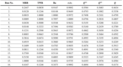
Table 5. Normalized decision matrix for Example 2

Run No. MRR TWR Ra r1/r2 Q(1) Q(2) Q

1. 0.2447 0.0830 0.9167 0.9892 0.5584 0.3683 0.4634

2. 0.0128 0.1246 0.8148 0.9649 0.4793 0.1882 0.3338

3. 0.0019 1.0000 1.0000 0.9972 0.7498 0.2101 0.4799

4. 0.0089 1.0000 0.7097 1.0000 0.6796 0.2818 0.4807

5. 0.0438 0.5000 0.5548 0.9632 0.5155 0.3288 0.4221

6. 0.0148 0.3333 0.7496 0.9583 0.5140 0.2439 0.3789

7. 0.1231 0.2500 0.5843 0.9872 0.4862 0.3650 0.4256

8. 0.8003 0.0663 0.3548 0.9786 0.5500 0.3684 0.4592

9. 0.3816 0.0474 0.5890 0.9791 0.4993 0.3195 0.4094

10. 0.6919 0.0415 0.3860 0.9865 0.5264 0.3233 0.4249

11. 0.1609 0.1659 0.4783 0.9855 0.4476 0.3349 0.3913

12. 0.0811 0.1246 0.4550 0.9759 0.4091 0.2588 0.3340

13. 0.3769 0.0368 0.5116 0.9817 0.4768 0.2890 0.3829

14. 0.5150 0.0331 0.6003 0.9809 0.5323 0.3167 0.4245

15. 1.0000 0.0166 0.4851 0.9755 0.6193 0.2976 0.4584

16. 0.4167 0.1246 0.3473 0.9892 0.4694 0.3654 0.4174

Table 6. Results of multi-response optimization for Example 2

Optimization method

Control factor

A B C D E F

Puhan et al. [21] 1 200 85 3.9226 15 300 (50)

WASPAS method 1 400 95 3.9226 15 400(37)

Table 7. Single response optimization results using WASPAS method

Response

Control factor

A B C D E F

Maximize MRR 7 300 85 3.9226 10 300 (50)

Minimize TWR 1 300 90 2.1419 15 300 (50)

Minimize Ra 1 300 90 2.1419 15 300 (50)

Maximize r1/r2 1 400 95 3.9226 15 400 (37)

3.2. Example 2

Puhan et al. [21] considered the machining

operation of AlSiC composite materials employing an EDM process. In EDM process, material from the workpiece surface is removed by controlled erosion through a series of electric sparks between the tool (electrode) and the workpiece. The thermal energy of the sparks thus leads to intense heat generation on the workpiece causing melting and vaporizing of the work material. As EDM is a complex electro-thermal process, it is quite difficult to establish the relationship between various EDM process parameters and responses. Using a design of experiments approach, the

effects of six EDM process parameters, like discharge current (A) (in A), pulse-on-time (B) (in µs), duty cycle (C) (in %), flushing pressure (D) (in Bar), SiC (E) (in wt%) and mesh size (F) (particle size in µm) on MRR (in mm3_{/min), tool wear rate (TWR) (in mm}3_/min),

surface roughness (Ra) (in µm) and circularity (r1/r2)

experimental plan along with the observed values of the responses is provided in Table 4. The values of this table are then linearly normalized in Table 5. From this table, it is observed that all the four responses are simultaneously optimized at experiment trial number 4, and for the optimal values of the responses (MRR = 0.316 mm3_{/min, TWR = 0.0037 mm}3_{/min, Ra = 6.2 µm}

and circularity = 0.9708), the best combination of the EDM process parameters can be set at discharge current = 1 A, pulse-on-time = 400 µs, duty cycle = 95%, flushing pressure = 3.9226 Bar, SiC = 15 wt% and mesh size 400(37).

Table 6 compares the optimal settings of the EDM process parameters as obtained using WASPAS method with those attained by Puhan et al. [21] while applying Taguchi method. At the optimal parametric settings, the response values were obtained as MRR = 14.376 mm3_{/min, TWR = 0.018mm}3_{/min, Ra = 3.043µm and}

circularity = 0.9700 [21].

In Table 7, the WASPAS method-based single response optimization results for the considered EDM process are shown, where the responses are separately optimized. It is quite interesting to note here that for attaining individual optimal values of the responses, separate parametric settings of the EDM process are required.

3.3. Example 3

Ultrasonic machining (USM) is an important non-traditional metal removal process for precision machining of hard and brittle materials. It is a non-thermal, non-chemical and non-electrical process, and creates no change in the metallurgical, chemical or physical properties of the workpiece material. Using Taguchi method and orthogonal array [4], Jadoun et al. [22] performed ultrasonic drilling operation on alumina-based ceramic materials, while considering five USM process parameters, such as workpiece material, tool material, grit size, power rating and slurry concentration. Each of those process parameters was set at three different levels, as shown in Table 8. In order to investigate the quality of the drilled holes, three responses were considered as hole oversize (HOC) (in mm), out-of-roundness (OOR) (in mm) and conicity (CC). All these three responses are of smaller-the-better type, thus always requiring minimum values. The detailed experimental plan, settings of the process parameters and observed values of the responses are shown in Table 9. The normalized data for this ultrasonic drilling operation is exhibited in Table 10. From this table, it becomes clearly evident that values of all the three quality characteristics are simultaneously minimized at experimental trial number 18. At the parametric combination of workpiece material (60% Al2O3),

tool material (TC), grit size (500), power rating (60%) and slurry concentration (25%), the minimum values of HOC (0.295 mm), OOR (0.240 mm) and CC (0.016) are concurrently achieved.

Table 8. Process parameters for ultrasonic drilling operation [22]

Process parameter Level 1 Level 2 Level 3

Workpiece material (A) 50% Al2O3

60% Al2O3

70% Al2O3

Tool material (B) HCS HSS TC

Grit size (C) 220 320 500

Power rating (D) 40% 50% 60% Slurry concentration (E) 25% 30% 35%

Table 9. Experimental plan and observations for ultrasonic drilling process [22]

Run No. Process parameter Response A B C D E HOS OOR CC

1. 1 1 1 1 1 0.382 0.450 0.048 2. 1 1 2 2 2 0.351 0.402 0.042 3. 1 1 3 3 3 0.156 0.368 0.037 4. 1 2 1 2 2 0.527 0.455 0.041 5. 1 2 2 3 3 0.339 0.283 0.041 6. 1 2 3 1 1 0.211 0.242 0.030 7. 1 3 1 3 3 0.566 0.445 0.039 8. 1 3 2 1 1 0.311 0.298 0.022 9. 1 3 3 2 2 0.309 0.307 0.014 10. 2 1 1 2 3 0.471 0.368 0.057 11. 2 1 2 3 1 0.307 0.345 0.046 12. 2 1 3 1 2 0.135 0.363 0.037 13. 2 2 1 3 1 0.463 0.442 0.050 14. 2 2 2 1 2 0.455 0.406 0.042 15. 2 2 3 2 3 0.311 0.391 0.035 16. 2 3 1 1 2 0.428 0.307 0.039 17. 2 3 2 2 3 0.390 0.284 0.024 18. 2 3 3 3 1 0.295 0.240 0.016 19. 3 1 1 3 2 0.645 0.405 0.068 20. 3 1 2 1 3 0.397 0.390 0.051 21. 3 1 3 2 1 0.075 0.350 0.044 22. 3 2 1 1 3 0.575 0.422 0.053 23. 3 2 2 2 1 0.313 0.425 0.045 24. 3 2 3 3 2 0.184 0.200 0.037 25. 3 3 1 2 1 0.523 0.359 0.065 26. 3 3 2 2 3 0.348 0.255 0.049 27. 3 3 3 1 3 0.249 0.212 0.026

last response (CC), its observed values are almost the same for both the set parametric combinations.

Table 10. Normalized data for Example 3

Run

No. HOS OOR CC Q

(1) _Q(2) _Q

1. 0.1963 0.4444 0.3333 0.3247 0.3076 0.3161 2. 0.2137 0.4975 0.3809 0.3640 0.3434 0.3537 3. 0.4808 0.5435 0.4324 0.4855 0.4835 0.4845 4. 0.1423 0.4396 0.3902 0.3240 0.2901 0.3071 5. 0.2212 0.7067 0.3902 0.4393 0.3937 0.4165 6. 0.3554 0.8264 0.5333 0.5717 0.5391 0.5554 7. 0.1325 0.4494 0.4102 0.3307 0.2902 0.3104 8. 0.2411 0.6711 0.7273 0.5465 0.4901 0.5183 9. 0.2422 0.6515 1.1426 0.6789 0.5654 0.6222 10. 0.1592 0.5435 0.2807 0.3278 0.2896 0.3087 11. 0.2443 0.5797 0.3478 0.3906 0.3666 0.3786 12. 0.5555 0.5510 0.4324 0.5129 0.5097 0.5113 13. 0.1620 0.4525 0.3200 0.3115 0.2863 0.2989 14. 0.1648 0.4926 0.3809 0.3461 0.3139 0.3300 15. 0.2416 0.5115 0.4571 0.4032 0.3835 0.3934 16. 0.1752 0.6515 0.4102 0.4123 0.3605 0.3864 17. 0.1923 0.7042 0.6667 0.5210 0.4486 0.4848 18. 0.2542 0.8333 1.0000 0.6958 0.5962 0.6460 19. 0.1163 0.4938 0.2353 0.2818 0.2382 0.2600 20. 0.1889 0.5128 0.3137 0.3384 0.3121 0.3253 21. 1.0000 0.5714 0.3636 0.6450 0.5923 0.6186 22. 0.1304 0.4739 0.3019 0.3020 0.2653 0.2837 23. 0.2396 0.4706 0.3555 0.3552 0.3423 0.3487 24. 0.4076 1.0000 0.4324 0.6133 0.5607 0.5870 25. 0.1434 0.5571 0.2461 0.3155 0.2699 0.2927 26. 0.2155 0.7843 0.3265 0.4421 0.3808 0.4114 27. 0.3012 0.9434 0.6154 0.6199 0.5592 0.5896

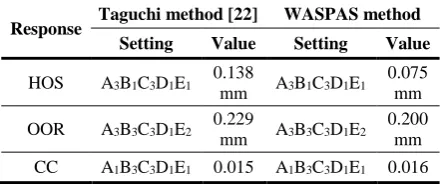
Table 11.Comparison of single response optimization results for Example 3

Response Taguchi method [22] WASPAS method Setting Value Setting Value

HOS A3B1C3D1E1 0.138

mm A3B1C3D1E1 0.075

mm OOR A3B3C3D1E2 0.229

mm A3B3C3D1E2 0.200

mm CC A1B3C3D1E1 0.015 A1B3C3D1E1 0.016

3.4. Example 4

Laser beam cutting is one of the predominant NTM processes, mostly used for generating complex shape features in different hard-to-machine materials, like metals, non-metals, ceramics, composites and super-alloys [23]. It is a thermal machining process, executed by moving a focused laser beam along the surface of the workpiece with constant distance, which generates a narrow cut kerf. The kerf entirely penetrates the mate-rial along the desired contour. During the machining

operation, a portion of the laser beam energy is absorbed at the end of the kerf. The absorbed energy heats and transforms the kerf volume into a molten, vaporized or chemically changed state to be subse-quently removed by a suitable coaxial gas jet. Among different solid state laser sources, Nd:YAG becomes the most popular industrial laser due to its various inherent advantages, like high laser beam intensity, low mean beam power, good focusing characteristics and narrow HAZ. It is observed that the machining performance of pulsed Nd:YAG laser depends on several process parameters, like pulse frequency, pulse energy, pulse width, cutting speed, assist gas type and its pressure. Thus, determination of the optimal settings of those process parameters is an important task for achieving enhanced machining performance.

Dubey and Yadava [23] performed experiments on a 200W pulsed Nd:YAG laser beam machining system with CNC work table and SUPERNI 718 (a Ni-based superalloy) was used in the experiments as the work material. Four process parameters, each set at three different levels, i.e. oxygen pressure (A) (2.0 kg/cm2_,

3.0 kg/cm2_{, 4.0 kg/cm}2_{), pulse width (B) (0.6 µs, 1.0 µs,}

1.4 µs), pulse frequency (C) (18 Hz, 23 Hz, 28 Hz) and cutting speed (D) (20 mm/min, 40 mm/min, 60 mm/min) were selected for the experimental purpose along with three quality characteristics (responses), i.e. kerf width (in mm), kerf deviation (in mm) and kerf taper (°). The detailed experimental plan, based on Taguchi’s L9 orthogonal array along with the allocation

of different process parameters as varying levels (shown in parentheses) is shown in Table 12. The measured dimensional values of the three considered responses are also provided in this table and it is worthwhile to mention here that all the three responses are of smaller-the-better (non-beneficial) type, thus always requiring lower values. The observed data are linearly normalized in Table 13 and it is found that for a λ value of 0.5, experiment trial number 1 provides the best machining performance of the Nd:YAG laser cutting process when equal importance is allocated to all the three responses. It thus signifies that for a process parameter combination of A1B1C1D1, i.e.

oxygen pressure = 2.0 kg/cm2_{, pulse width = 0.6 µs,}

pulse frequency = 18 Hz and cutting speed = 20 mm/min, the best performance of the said process can be attained. This parametric setting can achieve the process response values as kerf width = 0.2340 mm, kerf deviation = 0.0300 mm and kerf taper = 0.4092°. While applying Taguchi method and principal compo-nent analysis for this multi-response optimization problem, Dubey and Yadava [23] identified A1B1C2D1

as the best parametric combination. On the other hand, for the individual minimum values of the three responses, WASPAS method provides the settings of the process parameters as A1B1C2D1 (minimum kerf

width of 0.2340 mm), A3B3C2D1 (minimum kerf

deviation of 0.0300 mm) and A1B1C1D1 (minimum kerf

Table 12. Experimental observations for Nd:YAG laser cutting process [23]

Trial No.

Factor Kerf width (mm)

Kerf deviation

(mm)

Kerf taper (°) A B C D

1. 2.0 (1)

0.6 (1)

18 (1)

20

(1) 0.2340 0.0300 0.4092 2. 2.0

(1) 1.0 (2)

23 (2)

40

(2) 0.4060 0.0500 0.8185 3. 2.0

(1) 1.4 (3)

28 (3)

60

(3) 0.4160 0.1200 1.2278 4. 3.0

(2) 0.6 (1)

23 (2)

60

(3) 0.3280 0.0300 0.8185 5. 3.0

(2) 1.0 (2)

28 (3)

20

(1) 0.4380 0.0300 0.6139 6. 3.0

(2) 1.4 (3)

18 (1)

40

(2) 0.4380 0.1200 1.0231 7. 4.0

(3) 0.6 (1)

28 (3)

40

(2) 0.3900 0.0400 1.2278 8. 4.0

(3) 1.0 (2)

18 (1)

60

(3) 0.3800 0.0700 1.2278 9. 4.0

(3) 1.4 (3)

23 (2)

20

(1) 0.4640 0.0200 0.4092

response optimization problems, the individual parametric settings as A1B1C1D1, A3B1C2D1 and

A1B1C2D1, respectively, were determined [23]. It is

interesting to note that the parametric combinations A3B1C2D1 and A1B1C2D1 as derived in [23] for

optimization of the individual responses do not exist amongst the experimental trials of Table 12. So, the process engineer would have to conduct additional sets of experimentations to achieve the optimal response values which may incur extra machining time and

machining cost. The main advantage of WASPAS method as an effective optimization tool lies in the fact that it can be able to determine the optimal process parameter settings from the existing combinations, thus relieving the process engineer from conducting additional experiments. Table 14 provides the performance scores of the alternative trials for Nd:YAG laser cutting process for varying λ values, and it is observed that the ranking performance of WASPAS method remains quite stable over the changing λ values. When the value of λ is varied within a range of 0 to 1, experiment trail number 1 remains as the most preferred parametric setting for the Nd:YAG laser cutting process, followed by experiment trial number 9. Applying Eqs. (7)-(10), the optimal values of λ for all the experimental trials are evaluated in Table 15 and it becomes again evident that experiment trial number 1 provides the best parametric setting for simultaneous optimization of all the considered responses.

Table 13. Normalized data and results for Example 4

Trial No.

Kerf width

Kerf deviation

Kerf taper Q

(1) _Q(2) _Q

1. 1.0000 0.6667 1.0000 0.8888 0.8736 0.8812 2. 0.5763 0.4000 0.4999 0.4920 0.4867 0.4894 3. 0.5625 0.1667 0.3333 0.3541 0.3150 0.3345 4. 0.7134 0.6667 0.4999 0.6266 0.6195 0.6231 5. 0.5342 0.6667 0.6665 0.6224 0.6192 0.6208 6. 0.5342 0.1667 0.3999 0.3669 0.3290 0.3480 7. 0.6000 0.5000 0.3333 0.4777 0.4642 0.4709 8. 0.6158 0.2857 0.3333 0.4115 0.3885 0.4000 9. 0.5043 1.0000 1.0000 0.8347 0.7960 0.8153

Table 14. Effect of λ on ranking performance of WASPAS method

λ = 0 λ = 0.1 λ = 0.2 λ = 0.3 λ = 0.4 λ = 0.5 λ = 0.6 λ = 0.7 λ = 0.8 λ = 0.9 λ = 1.0

0.8736 0.8751 0.8766 0.8781 0.8797 0.8812 0.8827 0.8842 0.8857 0.8873 0.8888 0.4867 0.4872 0.4878 0.4883 0.4888 0.4894 0.4899 0.4904 0.4910 0.4915 0.4920 0.3150 0.3189 0.3228 0.3267 0.3306 0.3346 0.3385 0.3424 0.3463 0.3502 0.3541 0.6195 0.6202 0.6210 0.6217 0.6224 0.6231 0.6238 0.6245 0.6252 0.6259 0.6266 0.6192 0.6195 0.6199 0.6202 0.6205 0.6208 0.6211 0.6215 0.6218 0.6221 0.6224 0.3290 0.3328 0.3366 0.3404 0.3442 0.3480 0.3518 0.3555 0.3593 0.3631 0.3669 0.4642 0.4655 0.4669 0.4682 0.4696 0.4709 0.4723 0.4736 0.4750 0.4763 0.4777 0.3885 0.3908 0.3931 0.3954 0.3977 0.4000 0.4023 0.4046 0.4069 0.4092 0.4115 0.7960 0.7999 0.8037 0.8076 0.8115 0.8153 0.8192 0.8231 0.8269 0.8308 0.8347

3.5. Example 5

Wire electrical discharge machining (WEDM) is a special form of traditional EDM process in which the electrode is a continuously moving electrically conduc-tive wire (made of thin copper, brass or tungsten of diameter 0.05-0.3 mm). The movement of the wire is

immersed in a liquid dielectric (kerosene/deionized water) medium. These electrical discharges melt and vaporize minute amounts of work material, which are ejected and flushed away by the dielectric, leaving small craters on the workpiece.

Table 15. Determination of optimal λ values for Example 4

Trial No. σ

2_(Q

i(1)) σ2(Qi(2)) λ Score

1. 0.000679 0.000636 0.483634 0.8810 2. 0.000206 0.000197 0.489195 0.4893 3. 0.000126 0.000083 0.395340 0.3305 4. 0.000334 0.000320 0.488961 0.6230 5. 0.000326 0.000320 0.494868 0.6208 6. 0.000131 0.000090 0.407022 0.3444 7. 0.000200 0.000180 0.472709 0.4706 8. 0.000159 0.000126 0.441874 0.3987 9. 0.000626 0.000528 0.457466 0.8137

Table 16. Experimental plan and observations for WEDM process [24]

Run No.

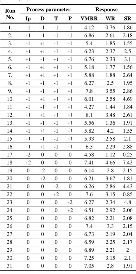
Process parameter Response Ip D T P VMRR WR SR

1. -1 -1 -1 -1 4.12 0.76 1.86 2. +1 -1 -1 -1 6.86 2.61 2.18 3. -1 +1 -1 -1 5.4 1.85 1.55 4. +1 +1 -1 -1 6.23 2.37 2.5 5. +1 -1 +1 -1 6.76 2.33 3.1 6. -1 +1 +1 -1 5.18 1.77 1.56 7. +1 +1 +1 -1 5.88 1.88 2.64 8. -1 -1 -1 +1 6.27 2.5 1.95 9. +1 -1 +1 +1 7.8 3.55 2.86 10. -1 +1 +1 +1 6.01 2.58 4.69 11. -1 -1 +1 +1 4.27 1.44 1.84

12. +1 +1 +1 +1 8.1 3.48 2.61

13. -1 -1 -1 +1 5.56 1.36 1.91 14. -1 +1 -1 +1 5.82 4.2 1.55 15. +1 -1 -1 +1 5.93 2.58 2.1 16. +1 +1 -1 +1 6.3 2.29 2.88 17. -2 0 0 0 4.58 1.12 0.25 18. +2 0 0 0 7.41 4.66 7.42 19. 0 -2 0 0 6.14 2.8 2.15 20. 0 +2 0 0 6.21 3.67 1.81 21. 0 0 -2 0 6.26 2.86 4.43 22. 0 0 +2 0 7.6 3.15 0.85 23. 0 0 0 -2 6.27 2.34 4.8 24. 0 0 0 +2 6.51 2.92 2.06 25. 0 0 0 0 6.82 2.21 2.08

26. 0 0 0 0 7.4 3.3 2.15

27. 0 0 0 0 6.73 2.19 2.04 28. 0 0 0 0 6.59 2.25 2.17

29. 0 0 0 0 6.89 2.21 2

30. 0 0 0 0 7.25 3.15 2.1

31. 0 0 0 0 7.05 2.8 1.91

Table 17. Normalized data for Example 5

Run

No. VMRR WR SR Q

(1) _Q(2) _Q

1. 0.5086 1.0000 0.1344 0.5476 0.4089 0.4783 2. 0.8469 0.2912 0.1147 0.4175 0.3047 0.3611 3. 0.6667 0.4108 0.1613 0.4129 0.3535 0.3832 4. 0.7691 0.3207 0.1000 0.3966 0.2911 0.3438 5. 0.8346 0.3262 0.0806 0.4137 0.2800 0.3469 6. 0.6395 0.4294 0.1602 0.4097 0.3531 0.3814 7. 0.7259 0.4042 0.0947 0.4082 0.3029 0.3556 8. 0.7741 0.3040 0.1282 0.4020 0.3113 0.3567 9. 0.9630 0.2141 0.0874 0.4214 0.2622 0.3419 10. 0.7420 0.2946 0.0533 0.3632 0.2267 0.2950 11. 0.5272 0.5278 0.1359 0.3969 0.3356 0.3663 12. 1.0000 0.2184 0.0958 0.4380 0.2755 0.3568 13. 0.6864 0.5588 0.1309 0.4587 0.3689 0.4138 14. 0.7185 0.1809 0.1613 0.3535 0.2758 0.3147 15. 0.7321 0.2946 0.1190 0.3819 0.2950 0.3384 16. 0.7778 0.3318 0.0868 0.3988 0.2820 0.3404 17. 0.5654 0.6786 1.0000 0.7479 0.7267 0.7373 18. 0.9148 0.1631 0.0337 0.3705 0.1713 0.2709 19. 0.7580 0.2714 0.1163 0.3819 0.2882 0.3350 20. 0.7667 0.2071 0.1381 0.3706 0.2800 0.3253 21. 0.7728 0.2657 0.0564 0.3650 0.2263 0.2956 22. 0.9383 0.2413 0.2941 0.4912 0.4053 0.4482 23. 0.7741 0.3248 0.0521 0.3836 0.2357 0.3097 24. 0.8037 0.2603 0.1213 0.3951 0.2939 0.3445 25. 0.8420 0.3439 0.1202 0.4353 0.3265 0.3809 26. 0.9136 0.2303 0.1163 0.4200 0.2903 0.3552 27. 0.8309 0.3470 0.1225 0.4334 0.3282 0.3808 28. 0.8136 0.3378 0.1152 0.4221 0.3164 0.3693 29. 0.8506 0.3439 0.1250 0.4398 0.3320 0.3859 30. 0.8951 0.2413 0.1190 0.4184 0.2952 0.3568 31. 0.8704 0.2714 0.1309 0.4242 0.3139 0.3690

Hewidy et al. [24] conducted experiments on a CNC WEDM machine using brass CuZn377 with 0.25mm in diameter as the wire and Inconel 601 as the work material. Four WEDM process parameters, each set at five different levels, i.e. peak current (Ip) (3A, 4A, 5A, 6A, 7A), duty factor (D) (0.375, 0.43, 0.50, 0.60, 0.75), wire tension (T) (7N, 7.5N, 8N, 8.5N, 9N) and water pressure (P) (3Mpa, 4Mpa, 5Mpa, 6Mpa, 7Mpa) were selected to study their effects on three responses, volumetric metal removal rate (VMRR, in mm3_/min),

simultaneous optimal values of all the three responses (VMRR = 4.58 mm3_{/min, WR = 1.12 and SR =}

0.25μm).

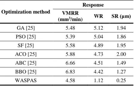
Mukherjee et al. [25] also considered the same WEDM process and applied six popular population-based non-traditional optimization algorithms, i.e. genetic algorithm (GA), particle swarm optimization (PSO), sheep flock algorithm (SF), ant colony optimization (ACO), artificial bee colony (ABC) and biogeography-based optimization (BBO) for single and multi-response optimization of this process. The results of the comparative studies between the optimal solutions obtained using those non-traditional optimization algorithms and those derived while applying WASPAS method for both single and multi-response optimization problems are provided in Table 18 and 19 respectively. Among the six non-traditional optimization algorithms applied for single as well as multi-response optimization of the WEDM process, it was observed that BBO algorithm had outperformed the others with respect to solution accuracy, computation time and consistency of the derived optimal solutions [25]. From the single response optimization results of Table 18, it is clear that WASPAS method provides smaller WR and SR values as compared to those obtained using BBO algorithm. The VMRR values are almost similar in both the cases. It is also interesting to observe that the optimal parametric settings as obtained using the six optimization algorithms did not at all belong to any of the initial experimental settings of the considered process parameters [25]. On the other hand, from the multi-response optimization results of Table 19, it is observed that for WASPAS method, the values of WR and SR are remarkably trimmed down, although there is no substantial increment in the VMRR value. The average computation time required for the six optimization algorithms was approximately measured as 15 s [25]. On the other hand, as all the calculation steps of WASPAS method are performed in EXCEL worksheet, its computation time is considerably less (approximately 5 s) as compared to the previously adopted algorithms.

Table 18. Comparison of single response optimization results for Example 5

Optimization method

Response VMRR

(mm3_/min) WR SR (μm) Hewidy et al. [24] 6.57 4.24 2.20

GA [25] 6.67 4.22 2.11

PSO [25] 6.87 4.19 1.98

SF [25] 7.03 4.18 1.75

ACO [25] 7.36 4.13 1.60

ABC [25] 7.87 4.09 1.35

BBO [25] 8.37 3.99 1.12

WASPAS 8.10 0.76 0.25

Table 19. Multi-response optimization results for Example 5

Optimization method

Response VMRR

(mm3_/min) WR SR (μm)

GA [25] 5.48 5.12 1.94

PSO [25] 5.39 5.04 1.86

SF [25] 5.58 4.89 1.95

ACO [25] 5.88 4.73 2.00

ABC [25] 6.66 4.51 1.49

BBO [25] 6.83 4.42 1.27

WASPAS 4.58 1.12 0.25

4. Conclusions

In this paper, an attempt is made to validate the applicability and effectiveness of WASPAS method as an effective optimization tool while solving five NTM process parameter selection problems. It is quite interesting to observe that WASPAS method can efficiently determine the optimal parametric combi-nations of the NTM processes for both single response as well as multi-response optimization problems. The main advantage of WASPAS method is that it can identify the optimal parametric combination of an NTM process from amongst the already conducted experimental trials, thus relieving the process engineer from performing additional experiments. As it is an aggregated method based on the concepts of WSM and WPM approaches, its solution accuracy is expected to be better than that of the single methods. Determining the optimal values of λ can further increase accuracy and effectiveness of this method in the decision-making process. Thus, its suitability as a simple and robust optimization tool is well proven to be successfully adopted for parametric optimization of other machining processes.

References

[1] P. C. Pandey, H. S. Shan. Modern Machining Processes. Tata McGraw-Hill Publishing Com. Ltd., New Delhi, 1981.

[2] E. J. Weller, M. Haavisto. Nontraditional Machining Processes. Society of Manufacturing Engineers, Michigan, 1984.

[3] V. K. Jain. Advanced Machining Processes. Allied Publishers Pvt. Limited., New Delhi, 2005.

[4] P. J. Ross. Taguchi Techniques for Quality Engineering. McGraw-Hill, Singapore, 1996.

[5] G. Derringer, R. Suich. Simultaneous optimization of several response variables. Journal of Quality Engineering, 1980, Vol. 12, No. 4, 214-219.

[6] K. R. MacCrimon. Decision Making among Multiple Attribute Alternatives: A Survey and Consolidated Approach. Rand Memorandum, RM-4823-ARPA, 1968.

methods: a decision-making paradox. Decision Support Systems, 1989, Vol. 5, No. 3, 303–312.

[8] R. V. Rao. Decision Making in the Manufacturing Environment using Graph Theory and Fuzzy Multiple Attribute Decision Making Methods. Springer-Verlag, London, 2007.

[9] D. W. Miller, M. K. Starr. Executive Decisions and Operations Research. Prentice-Hall, Inc., Englewood Cliffs, New Jersey, 1969.

[10] J. Šaparauskas, E. K. Zavadskas, Z. Turskis. Selection of facade’s alternatives of commercial and public buildings based on multiple criteria. International Journal of Strategic Property Management, 2011, Vol. 15, No. 2, 189–203.

[11] E. K. Zavadskas, Z. Turskis, J. Antucheviciene, A. Zakarevicius. Optimization of weighted aggregated sum product assessment. Elektronika ir Elektrotechnika, 2012, No. 6, 3–6.

[12] E. K. Zavadskas, J. Antucheviciene, J. Šaparauskas, Z. Turskis, Z. Multi-criteria assessment of facades’ alternatives: peculiarities of ranking methodology. Procedia Engineering, 2013, Vol. 57, 107–112. [13] E. K. Zavadskas, J. Antucheviciene, J. Saparauskas,

Z. Turskis. MCDM methods WASPAS and MULTIMOORA: verification of robustness of methods when assessing alternative solutions. Economic Computation and Economic Cybernetics Studies and Research, 2013, Vol. 47, No. 2, 5–20.

[14] S. Hashemkhani Zolfani, M. H. Aghdaie, A. Derakhti, E. K. Zavadskas, M. H. M. Varzandeh.

Decision making on business issues with foresight perspective; an application of new hybrid MCDM model in shopping mall locating. Expert Systems with Applications, 2013, Vol. 40, No. 17, 7111–7121. [15] T. Dėjus, J. Antuchevičienė. Assessment of health and

safety solutions at a construction site. Journal of Civil Engineering and Management, 2013, Vol. 19, No. 5, 728–737.

[16] M. Staniūnas, M. Medineckienė, E. K. Zavadskas,

D. Kalibatas. To modernize or not: ecological - economical assessment of multi-dwelling houses

modernization. Archives of Civil and Mechanical Engineering, 2013, Vol. 13, No. 1, 88–98.

[17] E. Šiožinyte, J. Antuchevičiene. Solving the problems of daylighting and tradition continuity in a reconstructed vernacular building. Journal of Civil Engineering and Management, 2013, Vol. 19, No. 6, 873–882.

[18] V. Bagočius, E. K. Zavadskas, Z. Turskis. Multi-criteria selection of a deep-water port in Klaipeda. Procedia Engineering, 2013, Vol. 57, 144–148. [19] S. Chakraborty, E. K. Zavadskas. Applications of

WASPAS method in manufacturing decision making. Informatica, 2014, Vol. 25, No. 1, 1–20.

[20] B. R. Sarkar, B. Doloi, B. Bhattacharyya. Parametric analysis of electrochemical discharge machining of silicon nitride ceramics. International Journal of Advanced Manufacturing Technology, 2006, Vol. 28, No. 9–10, 873–881.

[21] D. Puhan, S. S. Mahapatra, J. Sahu, L. Das. A hybrid approach for multi-response optimization of non-conventional machining on AlSiCp MMC. Measure-ment, 2013, Vol. 46, No. 9, 3581–3592.

[22] R. S. Jadoun, P. Kumar, B. K. Mishra. Taguchi’s optimization of process parameters for production accuracy in ultrasonic drilling of engineering ceramics. Production Engineering: Research and Development, 2009, Vol. 3, No. 3, 243–253.

[23] A. K. Dubey, V. Yadava. Multi-objective optimization of Nd:YAG laser cutting of nickel-based superalloy sheet using orthogonal array with principal component analysis. Optics and Lasers in Engineering, 2008, Vol. 46, No. 2, 124–132.

[24] M. S. Hewidy, T. A. El-Taweel, M. F. El-Safty.

Modelling the machining parameters of wire electrical discharge machining of Inconel 601 using RSM. Journal of Materials Processing Technology, 2005, Vol. 169, No. 2, 328–336.

[25] R. Mukherjee, S. Chakraborty, S. Samanta.

Selection of wire electrical discharge machining process parameters using non-traditional optimization algorithms. Applied Soft Computing, 2012, Vol. 12, No. 8, 2506–2516.