https://doi.org/10.5194/gmd-12-387-2019 © Author(s) 2019. This work is distributed under the Creative Commons Attribution 4.0 License.
Description and evaluation of the Community
Ice Sheet Model (CISM) v2.1
William H. Lipscomb1,2, Stephen F. Price1, Matthew J. Hoffman1, Gunter R. Leguy2, Andrew R. Bennett3,4, Sarah L. Bradley5, Katherine J. Evans3, Jeremy G. Fyke1,6, Joseph H. Kennedy3, Mauro Perego7,
Douglas M. Ranken1, William J. Sacks2, Andrew G. Salinger7, Lauren J. Vargo1,8, and Patrick H. Worley3 1Los Alamos National Laboratory, Los Alamos, NM 87544, USA
2Climate and Global Dynamics Laboratory, National Center for Atmospheric Research, Boulder, CO 80305, USA 3Computational Earth Sciences Group, Oak Ridge National Laboratory, Oak Ridge, TN 37830, USA
4University of Washington, Seattle, WA 98195, USA
5Delft University of Technology, Delft, 2600 AA, the Netherlands 6Associated Engineering Group, Ltd., Vernon, BC V1T 9P9, Canada
7Center for Computing Research, Sandia National Laboratories, Albuquerque, NM 87185, USA 8Victoria University of Wellington, Wellington 6140, New Zealand
Correspondence:William H. Lipscomb ([email protected]) Received: 18 June 2018 – Discussion started: 18 July 2018
Revised: 17 December 2018 – Accepted: 3 January 2019 – Published: 22 January 2019
Abstract.We describe and evaluate version 2.1 of the Com-munity Ice Sheet Model (CISM). CISM is a parallel, 3-D thermomechanical model, written mainly in Fortran, that solves equations for the momentum balance and the thick-ness and temperature evolution of ice sheets. CISM’s veloc-ity solver incorporates a hierarchy of Stokes flow approxi-mations, including shallow-shelf, depth-integrated higher or-der, and 3-D higher order. CISM also includes a suite of test cases, links to third-party solver libraries, and parameteri-zations of physical processes such as basal sliding, iceberg calving, and sub-ice-shelf melting. The model has been veri-fied for standard test problems, including the Ice Sheet Model Intercomparison Project for Higher-Order Models (ISMIP-HOM) experiments, and has participated in the initMIP-Greenland initialization experiment. In multimillennial sim-ulations with modern climate forcing on a 4 km grid, CISM reaches a steady state that is broadly consistent with ob-served flow patterns of the Greenland ice sheet. CISM has been integrated into version 2.0 of the Community Earth Sys-tem Model, where it is being used for Greenland simulations under past, present, and future climates. The code is open-source with extensive documentation and remains under ac-tive development.
1 Introduction
Larour et al., 2012), the Penn State Model (Pollard and De-Conto, 2012), BISICLES (Cornford et al., 2013), Elmer-Ice (Gagliardini et al., 2013), and MPAS-Albany Land Elmer-Ice (MALI; Tezaur et al., 2015; Hoffman et al., 2018). Higher-order models have performed well for standard test cases (Pattyn et al., 2008; Pattyn et al., 2012) and have been ap-plied to many scientific problems.
Here, we describe and evaluate the Community Ice Sheet Model (CISM) version 2.1, a higher-order model that evolved from the Glimmer model (Rutt et al., 2009). The cur-rent name reflects the model’s evolution as a component of the Community Earth System Model (CESM; Hurrell et al., 2013). Like Glimmer, CISM is written mainly in Fortran 90 and its extensions, to maximize efficiency and to simplify coupling to climate models. Glimmer, however, is a serial SIA model, whereas CISM is a parallel model that solves not only the SIA but also higher-order Stokes approximations.
CISM development was guided by the following goals: – The model should be well documented and easy to
in-stall and run on a variety of platforms, ranging from lap-tops to local clusters to high-performance supercomput-ers.
– It should solve a range of Stokes approximations, in-cluding the SIA, SSA, and higher-order approxima-tions. Velocity solvers for these approximations are in-cluded in a new dynamical core called Glissade. (The dynamical core, or “dycore”, is the part of the model that solves equations for conservation of mass, energy, and momentum.)
– It should remain backward-compatible with Glimmer, allowing continued use of the older Glide SIA dycore. – It should be well verified for standard test cases such
as the Ice Sheet Model Intercomparison Project for Higher-Order Models (ISMIP-HOM) (Pattyn et al., 2008), with a user-friendly verification framework. – It should run efficiently – supporting whole-ice-sheet
applications even on small platforms – and should scale to hundreds of processor cores, enabling century- to millennial-scale simulations with higher-order solvers at grid resolutions of ∼5 km or finer.
– It should support not only stand-alone ice sheet simu-lations but also coupled applications in which fields are exchanged with a global climate or Earth system model (CESM in particular).
– It should support simulations of the Greenland ice sheet, a scientific focus of CESM. Support for Antarctic appli-cations is deferred to future model releases and publica-tions.
– The code should be open-source, with periodic public releases.
Many of these features were present in CISM v.2.0, which was released in 2014 (Price et al., 2015).
Changes between versions 2.0 and 2.1 have been made primarily to support robust, accurate, and efficient Green-land ice sheet simulations, both as a stand-alone model and in CESM. These changes include a depth-integrated higher-order velocity solver (Sect. 3.1.4), new parameterizations of basal sliding (Sect. 3.4), iceberg calving (Sect. 3.5), and sub-ice-shelf melting (Sect. 3.6), a new build-and-test structure (Sect. 4.6), and many improvements in model numerics.
We begin with an overview of CISM, including the core model and its testing and coupling infrastructure (Sect. 2). We then describe the model dynamics and physics, focusing on the new Glissade dycore (Sect. 3). To verify the model, we present results from standard test cases (Sect. 4). We then present results from long spin-ups of the Greenland ice sheet, with and without floating ice shelves (Sect. 5). Finally, we summarize the model results and suggest directions for future work (Sect. 6).
2 Model overview
CISM is a numerical model – a collection of software li-braries, utilities, and drivers – used to simulate ice sheet evolution. It is modular in design and is coded mainly in standard-compliant Fortran 90/95. CISM consists of several components:
cism_driver is the high-level driver (i.e., the executable) that is used to run the stand-alone model in all config-urations, including idealized test cases with simplified climate forcing, as well as model runs with realistic ge-ometry and climate forcing data.
Glide is the serial dycore based on shallow-ice dynamics. Glide solves the governing conservation equations and computes ice velocities, internal ice temperature, and ice geometry evolution. Apart from minor changes, this is the same dycore used in Glimmer and described by Rutt et al. (2009). It will not be discussed further here. Glissade is the dycore that solves higher-order
approxima-tions of the Stokes equaapproxima-tions for ice flow. Glissade, un-like Glide, is fully parallel in order to take advantage of multiprocessor, high-performance architectures. It is described in detail in Sect. 3.
Glint is the original climate model interface for Glimmer. Glint allows the core ice sheet model to be coupled to a global climate model or any other source of time-varying climate data on a lat–long grid. Glint computes the surface mass balance (SMB) on the ice sheet grid using a positive-degree-day (PDD) scheme.
remapping and downscaling between general land-surface grids and ice sheet grids, and thus is able to send CISM an SMB that is already downscaled. The Glad in-terface simply sends and receives fields on the ice sheet grid, accumulating and averaging as needed based on the ice dynamic time step and the coupling interval. Test cases are provided for the Glide and Glissade
dynam-ical cores. These are used to confirm that the model is working as expected and to provide a range of simple model configurations from which new users can learn about model options and create their own configura-tions. CISM test cases are described in Sect. 4.
Shared code consists of modules shared by different parts of the code. Examples include modules for defining de-rived types, physical constants, and model parameters, and modules that parse CISM configuration files and handle data input/output (I/O).
In order to reduce development effort, CISM runs on a structured rectangular grid and thus lacks the flexibility of models that run on variable-resolution or adaptive meshes (e.g., ISSM and BISICLES). Although CISM includes sev-eral common Stokes approximations, it does not solve the more complex “full Stokes” equations (Pattyn et al., 2008).
CISM is distributed as source code and therefore requires a reasonably complete build environment to compile the model. For UNIX- and LINUX-based systems, the CMake (http://www.cmake.org/, last access: 20 January 2019) sys-tem is used to build the model. Sample build scripts for a number of standard architectures are included, as are working build scripts for a number of high-performance-computing architectures including Cheyenne (NCAR Com-putational and Information Systems Laboratory), Titan (Oak Ridge Leadership Computing Facility), Edison (National En-ergy Research Scientific Computing Center), and Cartesius (the Dutch national supercomputer).
The source code can be obtained by downloading a re-leased version from the CISM website or by cloning the code from a public git repository; see Sect. . In either case, a Fortran 90 compiler is required. Other software dependen-cies include the NetCDF library (https://www.unidata.ucar. edu/software/netcdf/, last access: 20 January 2019) (used for data I/O) and a Python (http://www.python.org, last access: 20 January 2019) distribution (used to analyze dependencies and to automatically generate parts of the code) with sev-eral specific Python modules. Parallel builds require Mes-sage Passing Interface (MPI), and users desiring access to Trilinos packages (Heroux et al., 2005) will need to build Trilinos and then link it to CISM. Finally, CMake and Gnu Make are needed to compile the code and link to the vari-ous third-party libraries. The CISM documentation contains detailed instructions for downloading and building the code. CISM is run by specifying the names of the executable (usuallycism_driver) and a configuration file. Typically, the
configuration file includes the input and output filenames, the grid dimensions, the time step and length of the run, the dy-core (Glide or Glissade), and various options and parameter values appropriate for a given application. If not set in the config file, each option or parameter takes a default value. Supported options are described in the model documentation. Multiple input, forcing, and output files can be specified, containing any subset of a large number of global scalars and fields (1-D, 2-D, and 3-D). If a given field is “loadable” and is present in the input file, it is read automatically at startup; otherwise, it is set to a default value. Loadable fields in-clude the initial ice thickness and temperature, bedrock to-pography, surface mass balance, surface air temperature, and geothermal heat flux. Forcing files are input files that are read at every time step (not just at initialization) so that time-dependent forcing can be applied during a simulation.
Each output file includes a user-chosen set of variables (listed in the configuration file) and can contain multiple time slices, written at any frequency. A special kind of I/O file is the restart file, which includes all the fields needed to restart the model exactly. Whatever configuration options are cho-sen, model results are exactly reproducible (i.e., bit for bit) for a given computer platform and processor count, regard-less of how many times a simulation is stopped and restarted. Some basic information is sent to standard output during the run, and more verbose output is written at regular inter-vals to a log file. The log file lists the options and parame-ter values chosen for the run and also notes the simulation time when CISM reads or writes I/O. In addition, the log file includes diagnostic information about the global state of the model (e.g., the total ice area and volume, total surface and basal mass balance, and maximum surface and basal ice speeds), along with vertical profiles of ice speed and temper-ature for a user-chosen grid point.
CISM2.1 has been implemented in CESM version 2.0, re-leased in June 2018. Earlier versions of CESM supported one-way forcing of the Greenland ice sheet (using SIA dy-namics) by the SMB computed in CESM’s land model (Lip-scomb et al., 2013). CESM2.0 extends this capability by sup-porting conservative, interactive coupling between ice sheets and the land and atmosphere. Coupling of ice sheets with the ocean is not yet supported but is under development. CESM2.0 does not have an interactive Antarctic ice sheet, in part because of the many scientific and technical issues as-sociated with ice sheet–ocean coupling. However, CISM2.1 includes many of the features needed to simulate marine ice sheets, and a developmental model version (including a grounding-line parameterization to be included in a near-future code release) has been used for Antarctic simulations.
3 Model dynamics and physics
mo-mentum (i.e., an appropriate approximation of Stokes flow), mass, and internal energy. Glissade numerics differ substan-tially from Glide numerics:
– Velocity: Glide solves the SIA only, but Glissade can solve several Stokes approximations, including the SIA, SSA, a depth-integrated higher-order approximation based on Goldberg (2011), and a 3-D higher-order ap-proximation based on Blatter (1995) and Pattyn (2003). Glide uses finite differences, whereas the Glissade ve-locity solvers use finite-element methods.
– Temperature: To evolve the ice temperature, Glide solves a prognostic equation that incorporates horizon-tal advection as well as vertical heat diffusion and in-ternal dissipation. In Glissade, temperature advection is handled by the transport scheme, and a separate module solves for vertical diffusion and internal dissipation in each column.
– Mass and tracer transport: Glide solves an implicit diffusion equation for mass transport, incorporating shallow-ice velocities. Glissade solves explicit equa-tions for horizontal transport of mass (i.e., ice thick-ness) and tracers (e.g., ice temperature) using either an incremental remapping scheme (Lipscomb and Hunke, 2004) or a simpler first-order upwind scheme. Hori-zontal transport is followed by vertical remapping to terrain-following sigma coordinates.
Glissade numerics are described in detail below. 3.1 Velocity solvers
Glissade computes the ice velocity by solving approximate Stokes equations, given the surface elevation, ice thick-ness, ice temperature, and relevant boundary conditions. Sec-tion 3.1.1 describes the soluSec-tion method for the Blatter– Pattyn (BP; Blatter, 1995; Pattyn, 2003) approximation, which is the most sophisticated and accurate solver in CISM. Subsequent sections discuss simpler approximations. 3.1.1 Blatter–Pattyn approximation
The basic equations of the Blatter–Pattyn approximation are
∂ ∂x
2η
2∂u
∂x+ ∂v ∂y
+ ∂
∂y
η
∂u ∂y+
∂v ∂x
+ ∂
∂z
η∂u ∂z
=ρig
∂s ∂x, ∂
∂y
2η
2∂v
∂y+ ∂u ∂x
+ ∂
∂x
η
∂u
∂y+ ∂v ∂x
+ ∂
∂z
η∂v ∂z
=ρig
∂s
∂y, (1)
whereuandvare the components of horizontal velocity,η
is the effective viscosity, ρi is the density of ice (assumed
Table 1.Model variables defined in the text.
Variables Definition
A Temperature-dependent rate factor B Surface mass balance
Bb Basal mass balance b Ice sheet bed elevation c Lateral calving rate Fd Diffusive heat flux Fg Geothermal heat flux Ff Frictional heat flux H Ice thickness
Heff Effective thickness at calving front Hf Flotation thickness
N Effective pressure P0 Full overburden pressure p Pressure at lateral boundaries s Surface elevation
T Ice temperature
Tf Ice temperature at floating lower surface Tpmp Pressure melting point temperature T? Absolute temperature corrected forTpmp u Horizontal ice velocity component ub Basalu
v Horizontal ice velocity component vb Basalv
W Water depth
β Basal traction parameter
βeff Effective basal traction parameter (DIVA) η Effective viscosity
˙
e Effective strain rate
˙
ij Strain rate tensor σ Vertical sigma coordinate
τb Basal shear stress τij Deviatoric stress tensor τe Effective stress τc Yield stress
τec Effective calving stress 8 Rate of internal heating φ Till friction angle
constant),gis gravitational acceleration,sis the surface ele-vation, andx, y, zare 3-D Cartesian coordinates. These and other variables and parameters used in CISM are listed in Ta-bles 1 and 2 for reference. In each equation, the three terms on the left-hand side (LHS) describe gradients of longitudinal stress, lateral shear stress, and vertical shear stress, respec-tively, and the right-hand side (RHS) gives the gravitational driving force. The longitudinal and lateral shear stresses to-gether are sometimes called membrane stresses (Hindmarsh, 2006). Neglecting membrane stress gradients leads to the much simpler SIA, and neglecting vertical shear stress gradi-ents leads to the SSA.
Table 2.Model constant and parameter values used for simulations described in the text. The calving and sub-shelf melting parameters are used only for simulations with ice shelves; other parameters are used for all Greenland simulations.
Parameters Value Units Definition
g 9.81 m s−2 Gravitational acceleration ci 2009 J kg−1K−1 Specific heat of ice ki 2.1 W m−1K−1 Thermal conductivity of ice L 335 J kg−1 Latent heat of melting ρi 917 kg m−3 Ice density
ρo 1026 kg m−3 Ocean water density ρw 1000 kg m−3 Fresh water density
n 3 – Glen flaw low exponent
q 0.5 – Exponent for pseudo-plastic sliding u0 100 m yr−1 Velocity scale for pseudo-plastic sliding φmax 40 ◦ Maximum bed angle for pseudo-plastic sliding φmin 5 ◦ Minimum bed angle for pseudo-plastic sliding bmax 700 m Upper bed limit for pseudo-plastic sliding bmin −700 m Lower bed limit for pseudo-plastic sliding δ 0.02 – Minimum effective pressure relative to overburden Cd 0.001 m yr−1 Till drainage rate
Wmax 2 m Maximum till water depth N0 1000 Pa Reference effective pressure
e0 0.69 – Void ratio at reference effective pressure CC 0.12 – Till compressibility
τc 106 Pa Yield stress for cliff limiting kτ 0.0025 m yr−1Pa−1 Empirical constant for calving w2 25 – Empirical constant for calving Hcmin 75 m Minimum thickness for calving tc 1 years Calving timescale
z0 −200 m Neutral elevation for sub-shelf melting Bfrzmax 3 m yr−1 Maximum sub-shelf freezing rate zmaxfrz −100 m yr−1 Elevation for maximum sub-shelf freezing Bmltmax 100 m yr−1 Maximum sub-shelf melting rate
zmaxfrz −500 m yr−1 Elevation for maximum sub-shelf melting H0 20 m Length scale for reducing melt in shallow cavities
based on a terrain-following sigma coordinate system, with
σ =(s−z)/H, whereHis the ice thickness. Each cell layer is treated as a 3-D hexahedral element with eight nodes. (In other words, cells and vertices are defined to lie in the map plane, whereas elements and nodes live in 3-D space.) Scalar 2-D fields such as H ands are defined at cell centers, and 3-D scalars such as the ice temperatureT lie at the centers of elements. Gradients of 2-D scalars (e.g., the surface slope
∇s) live at vertices. The velocity components u andv are 3-D fields defined at nodes.
For problems on multiple processors, a cell or vertex (and the associated elements and nodes in its column) may be either locally owned or part of a computational halo. Each processor is responsible for computing u and v at its cally owned nodes. Any cell that contains one or more lo-cally owned nodes and has H exceeding a threshold thick-ness (typically 1 m) is considered dynamically active, as are
the elements in its column. Likewise, any vertex of an active cell is active, as are the nodes in its column.
The effective viscosityηis defined in each active element by
η≡1
2A
−1
n ε˙
1−n n
e , (2)
whereAis the temperature-dependent rate factor in Glen’s flow law (Glen, 1955), andε˙eis the effective strain rate, given in the BP approximation by
˙
εe2= ˙εxx2 + ˙εyy2 + ˙εxxε˙yy+ ˙εxy2 + ˙ε2xz+ ˙εyz2 , (3) where the components of the symmetric strain rate tensor are
˙ εij =
1 2
∂u
i
∂xj +∂uj
∂xi
. (4)
The rate factorAis given by an Arrhenius relationship:
where T∗ is the absolute temperature corrected for the dependence of the melting point on pressure (T∗=T+
8.7×10⁻⁴(s−z), with T in Kelvin), a is a temperature-independent material constant from Paterson and Budd (1982), Q is the activation energy for creep, and R is the universal gas constant.
The coupled partial differential equations (PDEs) (1) are discretized using the finite-element method (e.g., Hughes, 2000; Huebner et al., 2001). This method is more often ap-plied to unstructured grids but was chosen for CISM’s rect-angular grid because of its robustness and natural treatment of boundary conditions (Dukowicz et al., 2010). The PDEs, with appropriate boundary conditions, are converted to a sys-tem of algebraic equations by dividing the full domain into subdomains (i.e., hexahedral elements), representing the ve-locity solution on each element, and integrating over ele-ments. The solution is approximated as a sum over trilinear basis functionsϕ. Each active node is associated with a basis function whose value isϕ=1 at that node, withϕ=0 at all other nodes. The solution at a point within an element can be expanded in terms of basis functions and nodal values:
u(x, y, z)=X n
ϕn(x, y, z)un,
v(x, y, z)=X n
ϕn(x, y, z)vn, (6)
where the sum is over the nodes of the element;unandvnare nodal values of the solution; andϕnvaries smoothly between 0 and 1 within the element.
Glissade’s finite-element scheme is formally equivalent to that described by Perego et al. (2012). Equation (1) can be written as
−∇·(2ηε˙1)= −ρig
∂s ∂x,
−∇·(2ηε˙2)= −ρig
∂s
∂y, (7)
where
˙ ε1=
2ε˙xx+ ˙εyy ˙ εxy
˙ εxz
, ε˙2=
˙ εxy ˙
εxx+2ε˙yy ˙ εyz
. (8)
Following Perego et al. (2012), these equations can be rewrit-ten in weak form. This is done by multiplying Eq. (7) by the basis functions and integrating over the domain, using inte-gration by parts to eliminate the second derivative:
Z
2ηε˙1(u, v)· ∇ϕ1d+ Z
0B
βuϕ1d0+ Z
0L
pn1ϕ1d0
+ Z
ρig
∂s
∂xϕ1d=0, Z
2ηε˙2(u, v)· ∇ϕ2d+ Z
0B
βuϕ2d0+ Z
0L
pn2ϕ2d0
+ Z
ρig
∂s
∂yϕ2d=0, (9)
whererepresents the domain volume,0Bdenotes the lower boundary,0Ldenotes the lateral boundary (e.g., the calving front of an ice shelf),βis a basal traction parameter,pis the pressure at the lateral boundary, andn1andn2are compo-nents of the normal to0L. These equations can also be ob-tained from a variational principle as described by Dukowicz et al. (2010). The four terms in Eq. (9) represent internal ice stresses, basal friction, lateral pressure, and the gravitational driving force, respectively.
At the basal boundary, we assume a friction law of the form
τb=βub, (10)
whereτbis the basal shear stress,ub=(ub, vb)is the basal velocity, andβ is a non-negative friction parameter that is defined at each vertex and can vary spatially. For some basal sliding laws (see Sect. 3.4),βdepends on the basal velocity. The lateral pressure p applies at marine-terminating boundaries. The net pressure is equal to the pressure directed outward from the ice toward the ocean by the ice, minus the (smaller) pressure directed inward from the ocean by the hy-drostatic water pressure. The outward pressure is found by integratingρig(s−z)dzfrom(s−H )tosand then dividing byH; it is given by
pout=
ρigH
2 . (11)
The inward pressure is found by integratingρogzdz(where
ρois the seawater pressure) from(s−H )to 0 and then di-viding by(H−s); it is given by
pin=
ρog(s−H )2
2H . (12)
Assuming hydrostatic balance (i.e., a floating margin), we haves−H=(ρi/ρo)H, in which case Eqs. (11) and (12) can be combined to give the net pressure
p=ρigH
2
1− ρi ρw
, (13)
directed from the ice to the ocean. However, Eqs. (11) and (12) are used in the code because they are valid at both grounded and floating marine margins. They are combined to give the net pressurep=pout−pinthat is integrated over vertical cliff faces0Lin Eq. (9).
The gravitational forcing terms require evaluating the gra-dients ∂s/∂x and ∂s/∂y at each active vertex. For vertex
(i, j ) (which lies at the upper right corner of cell (i, j )), these are computed using a second-order-accurate centered approximation:
s(i+1, j+1)+s(i+1, j )−s(i, j+1)−s(i, j )
21x , (14)
and similarly for ∂s/∂y. This is equivalent to computing
∂s/∂x at the edge midpoints adjacent to the vertex in they
direction, and then averaging the two edge gradients to the vertex. In some cases (e.g., near steep margins), Eq. (14) can lead to checkerboard noise (i.e., 2-D patterns of alternating positive and negative deviations in s at the grid scale), be-cause centered averaging ofspermits a computational mode. To damp this noise, Glissade also supports upstream gradient calculations that do not have this computational mode but are formally less accurate.
Equation (14) is ambiguous at the ice margin, where at least one of the four cells neighboring a vertex is ice-free. One option is to include all cells, including ice-free cells, in the gradient. This approach works reasonably well (albeit with numerical errors; see, e.g., Van den Berg et al., 2006) for land-based ice but can give large gradients and exces-sive ice speeds at floating shelf margins. A second option is to include only ice-covered cells in the gradient. For ex-ample, suppose cells(i, j )and(i, j+1)have ice, but cells
(i+1, j ) and(i+1, j+1)are ice-free. Then, lacking the required information to computex gradients at the adjacent edges, we would set∂s/∂x=0. With aygradient available at one adjacent edge, we would have∂s/∂y=(s(i, j+1)− s(i, j ))/(21y). This option works well at shelf margins but tends to underestimate gradients at land margins. A third, hy-brid option is to compute a gradient at edges where either (1) both adjacent cells are covered or (2) one cell is covered and lies higher in elevation than a neighboring ice-free land cell. Thus, gradients are set to zero at edges where an ice-covered cell (either grounded or floating) lies above ice-free ocean, or where an ice-covered land cell lies below ice-free land (i.e., a nunatak). Since this option works well for both land and shelf margins, it is the default.
GivenT,s,H, and an initial guess foruandv, the prob-lem is to solve Eq. (1) foruandvat each active node. This problem can be written as
Ax=b, (15)
or more fully,
Auu Auv Avu Avv
u v = bu bv . (16)
In Glissade,Ais always symmetric and positive definite. SinceAdepends (throughηand possiblyβ) onuandv, the problem is nonlinear and must be solved iteratively. For each nonlinear iteration, Glissade computes the 3-Dηfield based on the current guess for the velocity field and solves a linear problem of the form (16). Then,ηis updated and the process is repeated until the solution converges to within a given tolerance. This procedure is known as Picard iteration. Appendix A describes how the terms in Eq. (9) are summed over elements and assembled into the matrixAand
vectorb. Section 3.1.5 discusses solution methods for the in-ner linear problem and the outer nonlinear problem.
3.1.2 Shallow-ice approximation
The shallow-ice equations follow from the Blatter–Pattyn equations if membrane stresses are neglected. The SIA analogs of Eq. (1) are
∂ ∂z η∂u ∂z
=ρig
∂s ∂x, ∂ ∂z η∂v ∂z
=ρig
∂s
∂y. (17)
The SIA could be considered a special case of the Blatter– Pattyn equations and solved using the same finite-element methods, ignoring the horizontal stresses. With these meth-ods, however, each ice column cannot be solved indepen-dently, because each node is linked to its horizontal neigh-bors by terms that arise during element assembly. As a result, a finite-element-based SIA solver is not very efficient.
Instead, Glissade has an efficient local SIA solver. The solver is local in the sense thatuandv in each column are found independently ofuandvin other columns. It resem-bles Glide’s SIA solver as described by Payne and Dongel-mans (1997) and Rutt et al. (2009), except that Glide incor-porates the velocity solution in a diffusion equation for ice thickness, whereas Glissade’s SIA solver computes u and
v only, with thickness evolution handled separately as de-scribed in Sect. 3.3.
For small problems that can run on one processor, there is no particular advantage to using Glissade’s local SIA solver in place of Glide. Glide’s implicit thickness solver permits a longer time step and thus is more efficient for problems run in serial. For whole-ice-sheet problems, however, Glissade’s parallel solver can hold more data in memory and may have faster throughput, simply because it can run on tens to hun-dreds of processors.
3.1.3 Shallow-shelf approximation
The SSA equations can be derived by vertically integrating the BP equations, given the assumption of small basal shear stress and vertically uniform velocity. The shallow-shelf ana-log of Eq. (1) is
∂ ∂x
2ηH¯
2∂u ∂x+ ∂v ∂y + ∂ ∂y ¯ ηH ∂u ∂y + ∂v ∂x
=ρigH
∂s ∂x, ∂
∂y
2ηH¯ 2∂v ∂y+ ∂u ∂x + ∂ ∂x ¯ ηH ∂u ∂y + ∂v ∂x
=ρigH
∂s
∂y, (18)
whereη¯ is the vertically averaged effective viscosity, andu
equations in weak form resemble Eqs. (8) and (9) but with-out the vertical shear terms. Thus, the SSA matrix and RHS can be assembled using the methods described in Sect. 3.1.1 and Appendix A, using 2-D rectangular (instead of 3-D hex-ahedral) elements and omitting the vertical shear terms. The effective viscosity is defined as in Eq. (2) but with a vertically averaged flow factor and with Eq. (3) replaced by
˙
εe2= ˙εxx2 + ˙ε2yy+ ˙εxxε˙yy+ ˙εxy2 . (19) The element matrices are 2-D analogs of Eqs. (A3)–(A6), with vertical derivatives excluded.
3.1.4 Depth-integrated-viscosity approximation Goldberg (2011) derived a higher-order stress approximation that in most cases is similar in accuracy to BP but is much cheaper to solve, because (as with the SSA) the matrix sys-tem is assembled and solved in two dimensions. Since the stress balance equations use a depth-integrated effective vis-cosity in place of a vertically varying visvis-cosity, we refer to this scheme as a depth-integrated-viscosity approximation, or DIVA. Arthern and Williams (2017) used a similar model, also based on Goldberg (2011), to simulate ice flow in the Amundsen Sea sector of West Antarctica. To our knowl-edge, CISM is the first model to adapt this scheme for mul-timillennial whole-ice-sheet simulations. Here, we summa-rize the DIVA stress balance and describe Glissade’s solution method. Section 4.2 compares DIVA results to BP results for the ISMIP-HOM experiments (Pattyn et al., 2008).
Dukowicz et al. (2010) showed that the Blatter–Pattyn equations (Eq. 1) and associated boundary conditions can be derived by taking the first variation of a functional and set-ting it to zero. The functional includes terms that depend on the effective strain rate (Eq. 3), which can be written as
˙
εBP2 =u2x+vy2+uxvy+ 1
4 uy+vx 2 +1 4u 2 z+ 1 4v 2
z, (20) whereuxdenotes the partial derivative∂u/∂x, and similarly for other derivatives. Goldberg (2011) derived an alternate set of equations using a similar functional but with the horizontal velocity gradients in the effective strain rate replaced by their vertical averages:
˙
εDIVA2 = ¯u2x+ ¯vy2+ ¯uxv¯y+ 1
4 u¯y+ ¯vx 2 +1 4u 2 z+ 1 4v 2 z, (21) where
¯ u= 1
H s Z
b
u(z)dz, v¯= 1 H
s Z
b
v(z)dz. (22)
The resulting equations of motion, analogous to Eq. (1), are 1
H ∂ ∂x
2ηH¯
2∂u¯
∂x+ ∂v¯ ∂y + 1 H ∂ ∂y ¯ ηH
∂u¯ ∂y+
∂v¯ ∂x + ∂ ∂z η∂u ∂z
=ρig
∂s ∂x, 1 H ∂ ∂y 2ηH¯
2∂v¯
∂y+ ∂u¯ ∂x + 1 H ∂ ∂x ¯ ηH
∂u¯ ∂y+
∂v¯ ∂x + ∂ ∂z η∂v ∂z
=ρig
∂s
∂y, (23)
where the depth-integrated effective viscosity is given by
¯ η= 1
H s Z
b
η(z)dz. (24)
The vertical shear terms still containη(z).
Since the horizontal stress terms are depth-independent, Eq. (23) can be integrated in the vertical to give
∂
∂x
2ηH¯
2∂u¯
∂x+ ∂v¯ ∂y + ∂ ∂y ¯ ηH
∂u¯ ∂y +
∂v¯ ∂x
−βub
=ρigH
∂s ∂x, ∂
∂y
2ηH¯
2∂v¯
∂y+ ∂u¯ ∂x + ∂ ∂x ¯ ηH ∂u¯ ∂y +
∂v¯ ∂x
−βvb
=ρigH
∂s
∂y, (25)
where the boundary conditions atbandshave been used to evaluate the vertical stress terms, with a sliding law of the form Eq. (10). Equation (25) is equivalent to the SSA stress balance (Eq. 18), except for the addition of basal stress terms. Thus, the methods used to assemble and solve the SSA equa-tions can be applied to the DIVA equaequa-tions to find the mean velocity componentsu¯andv¯.
In order to solve Eq. (25), however, the basal stress terms must be rewritten in terms ofu¯ andv¯. Following Goldberg (2011), we show how this is done for thex component of velocity; theycomponent is analogous. Thexcomponent of Eq. (25) can be rearranged and divided byH:
βub H = 1 H ∂ ∂x 2Hη¯
2∂u¯
∂x+ ∂v¯ ∂y + 1 H ∂ ∂y Hη¯
∂u¯ ∂y+
∂v¯ ∂x
−ρig
∂s
∂x. (26)
From Eq. (23), the RHS of Eq. (26) is just−(ηuz)z, giving βub
H = −
∂ ∂z η∂u ∂z . (27)
Integrating Eq. (27) fromzto the surfacesgives
η∂u ∂z =
βub(s−z)
H . (28)
Dividing byηand integrating frombtozgivesu(z)in terms ofubandη(z):
u(z)=ub+
βub
H z Z
b
s−z0 η(z0) dz
0
Following Arthern et al. (2015), we can define some useful integralsFnas
Fn≡ s Z
b 1
η s−z
H n
dz. (30)
In this notation, the surface velocity is related to the bed ve-locity by
us=ub(1+βF1) . (31)
Integratingu(z)from the bed to the surface gives the depth-averaged mean velocityu¯:
¯
u=ub(1+βF2) . (32)
We can think of F2 as a depth-integrated inverse viscosity. The less viscous the ice, the greater the value ofF2, and the greater the difference betweenu¯andub.
Given Eq. (32), we can replaceβubandβvbin Eq. (25) withβeffu¯andβeffv¯, respectively, where
βeff=
β
1+βF2
. (33)
For a frozen bed (ub=vb=0, with nonzero basal stressτbx), theβubterm on the RHS of Eq. (29) is replaced byτbx, lead-ing to
¯
u=τbxF2. (34)
Then, the basal stress terms in Eq. (25) can be replaced by
βefffrzu¯andβefffrzv¯, where
βefffrz= 1 F2
. (35)
With these substitutions, Eq. (25) can be written in terms of mean velocitiesu¯andv¯and is fully analogous to the SSA.
In order to compute η¯, the effective viscosityη(z) must be evaluated at each level. We use Eq. (2) with the effective strain rate (Eq. 21). The horizontal terms inε˙DIVA2 are found using the mean velocities from the previous iteration. The vertical shear terms are computed using Eq. (28):
uz(z)=
τbx(s−z)
η(z)H , vz(z)=
τby(s−z)
η(z)H , (36)
where bothη(z)andτbare from the previous iteration. The DIVA solution procedure can be summarized as fol-lows:
1. Starting with the current guess for the velocity field
(u, v), assemble the DIVA solution matrix in analogy to the SSA solution matrix, with the following DIVA-specific computations:
– Computeη(z) using Eqs. (2), (21), and (36), and integrate to find the depth-averagedη¯.
– Evaluate numerically the vertical integrals in Eqs. (29) and (30).
– InterpolateF2to vertices and computeβeff. 2. Solve the matrix system foru¯andv¯.
3. Given(u,¯ v)¯ at each vertex, use Eq. (32) to find(ub, vb), and then use Eq. (29) to findu(z)at each level. 4. Iterate to convergence.
The code is initialized with(u, v)=0 everywhere, and there-after each iterated solution starts with(u, v)from the previ-ous time step.
DIVA assumes that horizontal gradients of membrane stresses are vertically uniform. It is less accurate than the BP approximation in regions of slow sliding and rough bed topography, where the horizontal gradients of membrane stresses vary strongly with height, and may also be less rate where vertical temperature gradients are large. The accu-racy of DIVA compared to BP is discussed in Sect. 4.2 with reference to the ISMIP-HOM benchmark experiments. 3.1.5 Solving the matrix system
After assembling the matrices and right-hand side vectors for the chosen approximation (SSA, DIVA, or BP), we solve the linear problem of Eq. (16). Glissade supports three kinds of solvers: (1) a native Fortran preconditioned conjugate gradi-ent (PCG) solver, (2) links to Trilinos solver libraries, and (3) links to the Sparse Linear Algebra Package (SLAP).
The native PCG solver works directly with the assembled matrices (Auu,Auv,Avu, andAvv) and the right-hand-side vectors (buandbv). Instead of converting to a sparse matrix format such as compressed row storage, Glissade maintains these matrices and vectors as structured rectangular arrays withiandj indices, so that they can be handled by CISM’s halo update routines. Each node location(i, j )(in 2-D) or
(i, j, k)(in 3-D) corresponds to a row of the matrix, and an additional indexm ranges over the neighboring nodes that can have nonzero terms in the columns of that row. The max-imum number of nonzero terms per row is 9 in 2-D and 27 in 3-D.
As described by Shewchuk (1994), the convergence rate of the PCG method depends on the effectiveness of the pre-conditioner (i.e., a matrixMwhich approximatesAand can be inverted efficiently). Glissade’s native PCG solver has two preconditioning options:
– diagonal preconditioning, in which M consists of the diagonal terms ofAand is trivial to invert, and
– shallow-ice-based preconditioning (for the BP approx-imation only). In this case,Mincludes only the terms inA that link a given node to itself and its neighbors above and below. Thus,Mis tridiagonal and can be in-verted efficiently. This preconditioner works well when the physics is dominated by vertical shear but not as well when membrane stresses are important. Since the preconditioner is local (it consists of independent col-umn solves), it scales well for large problems.
The Trilinos solver (Heroux et al., 2005) uses C++ pack-ages developed at Sandia National Laboratories. As de-scribed by Evans et al. (2012), an earlier version of CISM’s higher-order dycore, known as Glam, was parallelized and linked to Trilinos. The Trilinos links developed for Glam were then adapted for Glissade’s SSA, DIVA, and BP solvers. The CISM documentation gives instructions for building and linking to Trilinos and choosing appropriate solver settings.
SLAP is a set of Fortran routines for solving sparse sys-tems of linear equations. SLAP was part of Glimmer and is used to solve for thickness evolution and temperature ad-vection in Glide. It can also be used to solve higher-order systems in Glissade, using either GMRES or a biconjugate gradient solver. The SLAP solver, however, is a serial code unsuited for large problems.
The default linear solver is native PCG using the Chronopoulos–Gear algorithm. Although it has been found to run efficiently on platforms ranging from laptops to super-computers, its preconditioning options are limited, so con-vergence can be slow for problems with dominant membrane stresses (e.g., large marine ice sheets). SLAP solvers are gen-erally robust and efficient but are limited to one processor. Trilinos contains many solver options, but in tests to date – using a generalized minimal residual (GMRES) solver with incomplete lower–upper (ILU) preconditioning – it has been found to be slower than the native PCG solver because of the extra cost of setting up Trilinos data structures, and possibly the slower performance of C++ compared to Fortran for the solver.
The linear solver is wrapped by a nonlinear solver that does Picard iteration. Following each iteration, a new global matrix is assembled, using the latest velocity solution to com-pute the effective viscosity. Glissade then comcom-putes the new residual,r=b−Ax. If thel2norm of the residual, defined as
√
(r,r), is smaller than a prescribed tolerance threshold, the nonlinear system of equations is considered solved.
Other-wise, the linear solver is called again, until the solution con-verges or the maximum number of nonlinear iterations (typ-ically 100) is reached. The number of nonlinear iterations per solve – and optionally, the number of linear iterations per nonlinear iteration – is written to standard output. In the event of non-convergence, a warning message is written to output, but the run continues. In some cases, convergence may im-prove later in the simulation, or solutions may be deemed sufficiently accurate even when not fully converged. 3.2 Temperature solver
The thermal evolution of the ice sheet is given by
∂T ∂t =
ki
ρici
∇2T−u·∇T−w∂T ∂z +
8 ρici
, (37)
whereT is the temperature in◦C,u=(u, v)is the horizon-tal velocity,wis the vertical velocity,kiis the thermal con-ductivity of ice,ci is the specific heat of ice, ρi is the ice density, and8is the rate of heating due to internal defor-mation and dissipation. This equation describes the conser-vation of internal energy under horizontal and vertical dif-fusion (the first term on the RHS), horizontal and vertical advection (the second and third terms, respectively), and in-ternal heat dissipation (the last term). Unlike Glide, which solves this equation in a single calculation, Glissade divides the temperature evolution into separate advection and diffu-sion/dissipation components. The temperature module uses finite-difference methods to solve for vertical diffusion and internal dissipation in each ice column:
∂T ∂t =
ki
ρic
∂2T ∂z2 +
8 ρici
, (38)
as described in this section. The advective part of Eq. (37) is described in Sect. 3.3. Horizontal diffusion is assumed to be negligible compared to vertical diffusion, giving∇2T '∂2T
∂z2.
In Glissade’s vertical discretization of temperature, T is located at the midpoints of the(nz−1)layers, staggered rel-ative to the velocity. This staggering makes it easier to con-serve internal energy under transport, where the internal en-ergy in an ice column is equal to the sum over layers of
ρiciT 1z, with layer thickness 1z. The upper surface skin temperature is denoted byT0and the lower surface skin tem-perature byTnz, giving a total ofnz+1 temperature values in each column.
The following sections describe how the terms in Eq. (38) are computed, how the boundary conditions are specified, and how the equation is solved.
3.2.1 Vertical diffusion
Glissade uses a verticalσ coordinate, withσ≡(s−z)/H. Thus, the vertical diffusion terms can be written as
∂2T ∂z2 =
1
H2
∂2T
The central difference formulas for first derivatives at the up-per and lower interfaces of layerkare
∂T ∂σ σk
=Tk−Tk−1 eσk−eσk−1 ,
∂T ∂σ σ
k+1
=Tk+1−Tk e σk+1−eσk
, (40)
whereeσkis the value ofσat the midpoint of layerk, halfway betweenσk andσk+1. The second partial derivative, defined at the midpoint of layerk, is
∂2T ∂σ2
eσk =
∂T ∂σ
σk+1−
∂T ∂σ σk
σk+1−σk
. (41)
Inserting Eq. (40) into (41), we obtain the vertical diffusion term:
∂2T ∂σ2
eσk
= Tk−1
(eσk−eσk−1) (σk+1−σk)
−Tk
1
(eσk−eσk−1) (σk+1−σk)
+ 1
(eσk+1−eσk) (σk+1−σk)
+ Tk+1
(eσk+1−eσk) (σk+1−σk)
. (42)
3.2.2 Heat dissipation
In higher-order models, the internal heating rate8in Eq. (38) is given by the tensor product of strain rate and stress:
8= ˙εijτij, (43)
whereτij is the deviatoric stress tensor. The effective stress (cf. Eq. 3) is defined by
τe2=1
2τijτij. (44)
The stress tensor is related to the strain rate and the effective viscosity by
τij=2ηε˙ij. (45)
Dividing each side of Eq. (45) by 2η, substituting in Eq. (43), and using Eq. (44) gives
8=τ
2 e
η. (46)
Both terms on the RHS of Eq. (46) are available to the tem-perature solver, since the higher-order velocity solver com-putesηduring matrix assembly and diagnosesτefromηand
˙
εij at the end of the calculation.
3.2.3 Boundary conditions
The temperature T0 at the upper boundary is set to min(Tair,0), where the surface air temperature Tair is usu-ally specified from data or passed from a climate model. The diffusive heat flux at the upper boundary (defined as positive up) is
Fdtop= ki H
T1−T0 eσ1
, (47)
where the denominator contains just one term becauseσ0= 0.
The lower ice boundary is more complex. For grounded ice, there are three heat sources and sinks. First, the diffusive flux from the bottom surface to the ice interior (positive up) is
Fdbot= ki H
Tnz−Tnz−1 1−
eσnz−1
. (48)
Second, there is a geothermal heat fluxFgwhich can be pre-scribed as a constant (∼0.05 W m−2) or read from an input file. Finally, there is a frictional heat flux associated with basal sliding, given by
Ff=τb·ub, (49)
whereτb andub are 2-D vectors of basal shear stress and basal velocity, respectively. With a friction law given by Eq. (10), this becomes
Ff=β(u2b+v2b). (50)
If the basal temperature Tnz< Tpmp (where Tpmp is the pressure melting point temperature), then the fluxes at the lower boundary must balance:
Fg+Ff=Fdbot. (51)
In other words, the energy supplied by geothermal heating and sliding friction is equal to the energy removed by vertical diffusion. If, on the other hand,Tnz=Tpmp, then the net flux is nonzero and is used to melt or freeze ice at the boundary:
Mb=
Fg+Ff−Fdbot
ρiL
, (52)
whereMbis the melt rate andL is the latent heat of melt-ing. Melting generates basal water, which may either stay in place, flow downstream (possibly replaced by water from upstream), or simply disappear from the system, depending on the basal water parameterization. While basal water is present,Tnzis held atTpmp.
For floating ice, the basal boundary condition is simpler;
3.2.4 Vertical temperature solution Equation (38) can be discretized for layerkas
Tkn+1−Tkn
1t =
ki
ρiciH2 h
akTkn−1+1−(ak+bk)Tkn+1+bkTkn+1+1 i
+ 8k ρici
, (53)
where the coefficientsak andbk are inferred from Eq. (42), andnis the current time level. The vertical diffusion terms are evaluated at the new time level, making the discretization backward Euler (i.e., fully implicit) in time. Equation (53) can be rewritten as
−αkTkn−1+1+(1+αk+βk)Tkn+1−βkTkn+1+1 =Tkn+8k1t
ρici
, (54)
where
αk= kiak1t ρiciH2
, βk= kibk1t ρiciH2
. (55)
At the lower surface, we have either a temperature bound-ary condition (Tnz=Tpmp for grounded ice, orTnz=Tffor floating ice) or a flux boundary condition:
Ff+Fg−
ki
H
Tnzn+1−Tnzn+1−1
1− eσnz−1
=0, (56)
which can be rearranged to give
−Tnzn+1−1+Tnzn+1= Ff+Fg
H (1− eσnz−1) ki
. (57)
In each ice column, the above equations form a tridiagonal system that is solved forTk in each layer.
Occasionally, the solutionTk can exceedTpmpfor a given layer. If so, we setTk=Tpmpand use the extra energy to melt ice internally. This melt is assumed to drain immediately to the bed. If Eq. (52) applies, we computeMband adjust the basal water depth. When the basal water goes to zero, Tnz is set to the temperature of the lowest layer (less thanTpmp at the bed), so that the flux boundary condition will apply during the next time step.
3.3 Mass and tracer transport
The transport equation for ice thicknessHcan be written as
∂H
∂t +∇·(HU)=B, (58)
where U is the vertically averaged 2-D velocity and B is the total surface mass balance. This equation describes the conservation of ice volume under horizontal transport. With the assumption of uniform density, volume conservation is
equivalent to mass conservation. There is a similar conserva-tion equaconserva-tion for the internal energy in each ice layer:
∂(hT )
∂t +∇·(hTu)=0, (59)
wherehis the layer thickness,T is the temperature (located at the layer midpoint), and uis the layer-average horizon-tal velocity. (Vertical diffusion and internal dissipation are handled separately as described in Sect. 3.2.) If other tracers are present, their transport is described by conservation equa-tions of the same form as Eq. (59). Glissade solves Eqs. (58) and (59) in a coordinated way, one layer at a time. All trac-ers, including temperature, are advected using the same al-gorithm.
Glissade has two horizontal transport schemes: a first-order upwind scheme and a more accurate incremental remapping (IR) scheme (Dukowicz and Baumgardner, 2000; Lipscomb and Hunke, 2004). The IR scheme is the default. This scheme was first implemented in the Los Alamos sea ice model, CICE, and has been adapted for CISM. Since the scheme is fairly complex, we give a summary in Sect. 3.3.1 and refer the reader to the earlier publications for details.
After horizontal transport, the mass balance is applied at the top and bottom ice surfaces. The new vertical layers gen-erally do not have the desired spacing inσ coordinates. For this reason, a vertical remapping scheme is applied to trans-fer ice volume, internal energy, and other conserved quanti-ties between adjacent layers, thus restoring each column to the desiredσcoordinates while conserving mass and energy. (This is a common feature of arbitrary Lagrangian–Eulerian (ALE) methods.) Internal energy divided by mass gives the new layer temperatures, and similarly for other tracers. 3.3.1 Incremental remapping
The incremental remapping scheme has several desirable fea-tures:
– It conserves the quantities being transported (including mass and internal energy).
– It is non-oscillatory; that is, it does not create spurious ripples in the transported fields.
– It preserves tracer monotonicity. That is, it does not cre-ate new extrema in tracers such as temperature; the val-ues at timen+1 are bounded by the values at timen. Thus,T never rises above the melting point under ad-vection.
– It is second-order accurate in space and therefore is less diffusive than first-order schemes. The accuracy may be reduced locally to first order to preserve monotonicity. – It is efficient for large numbers of tracers. Much of the
The model’s upwind scheme, like IR, is conservative, non-oscillatory, and monotonicity preserving, but because it is first order it is highly diffusive.
The IR time step is limited by the requirement that trajec-tories projected backward from grid cell corners are confined to the four surrounding cells; this is what is meant by incre-mental as opposed to general remapping. This requirement leads to an advective Courant–Friedrichs–Lewy (CFL) con-dition,
max|u|1t
1x ≤1. (60)
The remapping algorithm can be summarized as follows: 1. Given mean values of the ice thickness and tracer fields
in each grid cell, construct linear approximations of these fields that preserve the mean. Limit the field gra-dients to preserve monotonicity.
2. Given ice velocities at grid cell vertices, identify depar-ture regions for the fluxes across each cell edge. Divide these departure regions into triangles and compute the coordinates of the triangle vertices.
3. Integrate the thickness and tracer fields over the depar-ture triangles to obtain the mass and energy transported across each cell edge.
4. Given this transport, update the state variables.
These steps are carried out for each ofnz−1 ice layers, where
nzis the number of velocity levels. 3.3.2 CFL checks
As mentioned above, the time step for explicit mass trans-port is limited by the advective CFL condition (Eq. 60). For ice flow parallel to∇s, ice thickness evolution is diffusive, giving rise to a diffusive CFL condition (Bueler, 2009):
(maxD)1t≤0.51x2, (61)
where D is the ice flow diffusivity. Flow governed by the shallow-ice approximation is subject to this diffusive CFL. The stability of Glissade’s BP, DIVA, and SSA solvers, how-ever, is limited by Eq. (60) in practice; Eq. (61) is too re-strictive. For this reason, Glissade checks for advective CFL violations at each time step. Optionally, the transport equa-tion can be adaptively subcycled within a time step to satisfy advective CFL. This can prevent the model from crashing, though possibly with a loss of accuracy.
3.4 Basal sliding
Glissade assumes a basal friction law of the form Eq. (10). Ifβ were independent of velocity, then Eq. (10) would be a simple linear sliding law. Allowingβ to depend on velocity allows more complex and physically realistic sliding laws. The following options are supported in CISM:
– Spatially uniformβ, possibly a large value that makes sliding negligible.
– No sliding, enforced by a Dirichlet boundary condition (ub=0) during finite-element assembly.
– A 2-Dβ field specified from an external file. Typically,
βis chosen at each vertex to optimize the fit to observed surface velocity.
– β is set to a large value where the bed is frozen (Tb<
Tpmp) and a lower value where the bed is thawed (Tb=
Tpmp).
– Power-law sliding, based on the sliding relation of Weertman (1957). Basal velocity is given by
ub=kτpbN−q, (62) whereN is the effective pressure (the difference be-tween the ice overburden pressureP0=ρigH and the basal water pressurepw) andkis an empirical constant. This can be rearranged to give
τb=k−1/pNq/pu1b/p. (63) – Plastic sliding, in which the bed deforms with a
speci-fied till yield stress.
– Coulomb friction as described by Schoof (2005), with notation and default values from Pimentel et al. (2010). The form of the sliding law is
τb=C|u|
1
n−1u
Nn
κ|u| +Nn 1n
, (64)
whereCis a constant,κ=mmax/(λmaxAb),mmaxis the maximum bed obstacle slope,λmaxis the wavelength of bedrock bumps, andAbis a basal flow-law parameter. Equation (64) has two asymptotic behaviors. In the inte-rior, where the ice is thick and slow-moving,κ|u| Nn
and the basal friction is independent ofN: τb≈C|u|
1
n−1u. (65)
The Coulomb-friction limit, where the ice is thin and fast-moving, we haveκ|u| Nn, giving
τb≈
C
κn1
N u
|u|. (66)
– Pseudo-plastic sliding, as described by Schoof and Hindmarsh (2010) and Aschwanden et al. (2013) and implemented in PISM. The basal friction law is τb= −τc
ub
|ub|1−quq0
where τc is the yield stress, q is a pseudo-plastic ex-ponent, and u0 is a threshold speed. This law incor-porates linear (q=1), plastic (q=0), and power-law (0< q <1) behavior in a single expression. The yield stress is given by τc=tan(φ)N, whereφ is a friction angle that can vary with bed elevation, resulting in a lower yield stress at lower elevations. This scheme has been shown to give a realistic velocity field for most of the Greenland ice sheet with tuning of just a few param-eters, instead of adjusting a basal friction parameter in every grid cell (Aschwanden et al., 2016).
The power-law, Coulomb-friction and pseudo-plastic slid-ing laws give lower basal friction and faster slidslid-ing as the ef-fective pressureN decreases from the overburden pressure. CISM offers several options for computingNat the bed:
– N=ρigH, the full overburden pressure. That is, the water pressurepw=0 at the bed.
– N is reduced as the basal water depth increases, reach-ing a small fraction of overburden pressure (typically
δ=0.02) when the water depth reaches a prescribed threshold.
– Following Leguy et al. (2014),N is reduced where the bed is below sea level, to account for partial or full con-nectivity of the basal water system to the ocean. The effective pressure is given by
N=ρigH
1−Hf H
p
, (68)
whereHf=max(0,−ρob/ρi)is the flotation thickness,
ρois seawater density,bis the bed elevation (negative below sea level), and 0≤p≤1. For p=0, there is no connectivity andN is the full overburden pressure. Forp=1, there is full connectivity, and the basal wa-ter pressure is equal to the ocean pressure at the same depth.
Glissade does not yet support sophisticated subglacial hy-drology. (The model of Hoffman and Price (2014) was imple-mented in serial in an earlier version of CISM but is not cur-rently supported.) The following (non-conserving) options are available for handling basal meltwater:
– All basal water immediately drains.
– Basal water depth is set to a constant everywhere, to forceT =Tpmp.
– Basal water depth is computed using a local till model, as described by Bueler and van Pelt (2015). In this model, water depthWevolves according to
∂W ∂t =
−Bb
ρw
−Cd, (69)
whereW is the water depth (capped at Wmax), Bb is the basal mass balance (negative for melting),ρwis the density of water, andCd is a fixed drainage rate. The effective pressureN is related to water depth by
N=min "
P0,N0 δP
0 N0
W/Wmax
10(e0/Cc)(1−W/Wmax) #
, (70)
wheree0is the void ratio at reference effective pressure
N0,Cc is the till compressibility, andδ is a scalar be-tween 0 and 1. Default values of these terms are taken from Bueler and van Pelt (2015). The effect of Eq. (70) is to driveN fromP0down toδP0asW increases from 0 toWmax.
3.5 Iceberg calving
Glissade supports several schemes for calving ice at marine margins. Two of these are very simple: (1) calve all float-ing ice and (2) calve ice where the bedrock (either the cur-rent bedrock or the bedrock toward which a viscous astheno-sphere is relaxing) lies below a prescribed elevation. In addi-tion, Glissade includes several new calving schemes: mask-based calving, thickness-mask-based calving, and eigencalving.
With mask-based calving, any floating ice that forms in cells defined by a calving mask is assumed to calve instantly. By default, the mask is based on the initial ice extent. Float-ing ice calves in all cells that are initially ice-free ocean, and thus the calving front cannot advance (but it can retreat). Al-ternatively, users can define a calving mask that is read at initialization.
Thickness-based calving is designed to remove floating ice that is thinner than a user-defined thickness,Hcmin. As dis-cussed by Albrecht et al. (2011), accurate thickness-based calving requires a subgrid-scale parameterization of the calv-ing front. Suppose, for example, thatHcmin=100 m, and an ice shelf with a calving front thicker than 100 m is advanc-ing. During the next time step, ice is transported to grid cells just downstream of the initial calving front. Typically, these cells haveH < Hcmin. If this thin ice immediately calves, the calving front cannot advance.
up-stream neighbor, formerly an active cell in the shelf interior, becomes an inactive CF cell.
Thickness-based calving is applied not to CF cells with
H < Hcmin but rather to cells with Heff< Hcmin. In other words, the CF thickness is inferred from the active cells just interior to the CF. WhereHeff< Hcmin, the effective rate of thickness change is given by
dHeff dt = −
Hcmin−Heff
tc
, (71)
where tc is a calving timescale. This effective rate is con-verted to dH /dt(i.e., the rate of ice volume change per unit cell area) as
dH
dt =min(H /Heff,1)
dHeff
dt . (72)
Glissade’s eigencalving scheme is related to the method described by Levermann et al. (2012) but differs in the de-tails. In the method of Levermann et al. (2012), the lateral calving rate is proportional to the product of the two eigen-values of the horizontal strain rate tensor, provided that both eigenvalues are positive. This scheme was tested in CISM but found to give noisy, erratic results. Instead, we compute the lateral calving ratecas
c=kττec, (73)
wherekτ is an empirical constant with units of m yr−1Pa−1, andτecis an effective calving stress defined by
τec2 =max(τ1,0)2+w2max(τ2,0)2. (74) Here,τ1andτ2are the eigenvalues of the 2-D horizontal de-viatoric stress tensor, andw2 is an empirical constant. The stresses τ1 and τ2 are positive when the ice is in tension;
τ1 corresponds to along-flow tension andτ2to across-flow tension. These stresses are computed for dynamically active cells and then are extrapolated to inactive neighbors. When
w2>1, across-flow tension drives calving more effectively than does along-flow tension, as is the case for the calving law of Levermann et al. (2012). Equation (74) is analogous to Eq. (6) in Morlighem et al. (2016) (in a calving law for Greenland’s Store Gletscher) but with stress replacing strain rate and with a weighting term added.
Using Eqs. (73) and (74), we can compute a lateral calving ratecfor each CF cell. The lateral calving rate is converted to a rate of volume change using
dH
dt = − Heffc
√
1x1y, (75)
where 1x and1y are the grid cell dimensions. Typically, CISM is run with1x=1y, but this is not a model require-ment.
Eigencalving, when applied on its own, can allow very thin ice to persist at the calving front where stresses are small. For
this reason, the eigencalving algorithm is automatically fol-lowed by thickness-based calving as described above, with
Hcminset to a value large enough to remove thin ice, where present, but not so large as to be the dominant driver of calv-ing.
An additional option related to calving is iceberg removal. An iceberg is defined as a connected region where every cell is floating and has no connection to grounded ice. Icebergs can be present in initial data sets and also can arise during simulations, depending on the calving scheme. Finding the velocity for such a region is an ill-posed problem, so it is best to remove icebergs as soon as they occur. This is done by first marking all the grounded ice cells, and then using a parallel flood-fill algorithm to mark every floating cell that is connected to a grounded cell. (That is, one could travel from a grounded cell to a given floating cell along a path at least one cell wide, without leaving the ice sheet.) Any unmarked floating cells then calve immediately.
Another option is to limit the thickness of ice cliffs, de-fined as grounded marine-based cells adjacent to ice-free ocean. Bassis and Walker (2012) pointed out that there is an upper thickness limit for marine-terminating cliffs of outlet glaciers. If the ice cliff sits more than∼100 m out of the wa-ter, the longitudinal stresses exceed the yield strength, and the ice will fail. The maximum stable thickness at the termi-nus is given by
Hmax=
τc
ρig
+ s
τ c
ρig 2
+ρo ρi
d2, (76)
whereτc∼1 MPa is the depth-averaged shear strength,d is the ocean depth, andρiandρoare densities of ice and seawa-ter. When cliff limiting is enabled in CISM, marine-grounded cells adjacent to ice-free ocean are limited toH≤Hmax, with any excess thickness added to the calving flux. This thinning mechanism does not trigger the rapid ice sheet retreat seen by Pollard et al. (2015) in Antarctic simulations that combined cliff failure with hydrofracture. CISM2.1 does not simulate hydrofracture or lateral cliff retreat.
3.6 Sub-shelf melting
By default, melting beneath ice shelves is set to zero. The fol-lowing simple options may be enabled for simulations with marine ice:
– Sub-shelf melting is set to a constant value for all float-ing ice.
– CISM reads in a 2-D field of basal melt rates and applies the prescribed rates to floating ice.
reference elevationz0, then increases linearly as a func-tion of depth. In shallow sub-shelf cavities, the melt rate is reduced to zero over a characteristic length scaleH0. The depth dependence is motivated by observations of temperature increasing with depth in polar regions but is not necessarily a realistic treatment of melting near grounding lines.
– The sub-shelf melt rate is a piecewise linear function of depth. Above a reference elevationz0there is freezing, and below z0 there is melting. Abovez0, the freezing rate increases linearly from 0 to Bfrzmax at zmaxfrz ; above
zmaxfrz , it is capped atBfrzmax. Similarly, belowz0, the melt rate increases linearly from 0 to Bmltmax at zmaxmlt; below
zmaxmlt, it is capped atBmltmax. In shallow cavities, the melt rate is reduced to zero over a scaleH0as for MISMIP+. Like the MISMIP+ parameterization, this is an ad hoc scheme that should be used with caution. More realistic treatments of sub-shelf melting are being actively devel-oped in the ocean and ice modeling communities (Asay-Davis et al., 2017).
Sub-shelf melting is applied only to cells that are floating based on the criterion b <−(ρi/ρo)H, whereb is bed el-evation (negative below sea level) and H is ice thickness. In partly filled cells at the calving front, basal melt is ap-plied to the effective thicknessHeffrather than the grid cell mean thicknessH (see Sect. 3.5). For example, a melt rate of 10 m yr−1applied to a cell that is 10 % full would reduce
H at a rate of only 1 m yr−1. Basal melting for grounded ice, including marine-based ice, is described in Sect. 3.2.3. 3.7 Isostasy
Isostatic adjustment is handled as in Rutt et al. (2009), with several options for the lithosphere and underlying astheno-sphere. The lithosphere can be described as either local (i.e., floating on the asthenosphere) or elastic (taking flex-ural rigidity into account). The asthenosphere is either fluid (reaching isostatic equilibrium instantaneously) or relaxing (responding to the load on an exponential timescale of sev-eral thousand years). The default, when isostasy is active, is an elastic lithosphere and relaxing asthenosphere.
In the elastic lithosphere calculation, data from many grid cells must be summed to compute the load in each location. For parallel runs, this is done by gathering data to one proces-sor to compute the load and then distributing the result to the local processors. This calculation scales poorly, but it is done infrequently (every∼100 model years) and therefore has a minimal computational cost at grid resolutions of∼5 km.
4 Model results: standard test cases
Test cases for CISM include (1) problems with analytic so-lutions, (2) standard experiments without analytic solutions
but for which community benchmarks are available, and (3) some CISM-specific experiments used for code devel-opment and testing. These tests are organized in directories, each of which includes a README file with instructions on running the test. Most tests have Python scripts that are used to set up the initial conditions and run the model, and some tests have an additional Python script to analyze and plot the output. Each test has a default configuration file, whose set-tings can be adjusted manually to make changes (e.g., swap-ping velocity solvers). Several tests are described below, with plots generated by Python scripts included in the code re-lease.
4.1 Halfar dome test
The Halfar test case describes the time evolution of a parabolic dome of ice (Halfar, 1983; Bueler et al., 2005). For a flat-bedded SIA problem without accumulation, this case has an analytic solution for the time-varying ice thickness. The SIA ice evolution equation can be written as
∂H
∂t =∇·(0H
n+2|∇H|n−1∇H ), (77)
wheren is the exponent in the Glen flow law, commonly taken as 3, and0=2A(ρg)n/(n+2)is a positive constant. Forn=3, the time-dependent solution is
H (t, r)=H0 t
0
t 19
1−
t 0
t 181 r
R0 !43
3 7
, (78)
where
t0= 1 180
7 4
3R4 0
H07, (79)
andH0andR0are the central dome height and dome radius, respectively, at timet=t0. As the dome evolves, the ice mar-gin advances and the thickness decreases. The test can be run using either Glide or Glissade solvers.
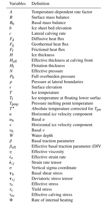
Figure 1a–c show Halfar dome results for the Glide solver withH0=500
√
2≈700 m,R0=15
√
2≈21 km, a grid res-olution of 2 km, and a time step of 5 years. The three panels show the modeled thickness, analytic thickness, and thick-ness difference, respectively, att=200 years. Differences are largest near the ice margin. The rms error in the solution is 6.43 m, with a maximum absolute error of 32.8 m.
Figure 1.Results from the Halfar dome test using SIA solvers from Glide(a, b, c)and Glissade(d, e, f).(a, d)Modeled ice thickness.(b, e)Analytic ice thickness.(c, f)Difference between modeled and analytic thickness.
can be attributed to the explicit transport solver (Sect. 3.3), which is less accurate for this problem than Glide’s implicit diffusion-based solver.
4.2 ISMIP-HOM tests
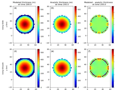
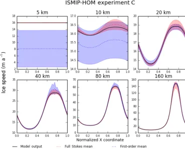
ISMIP-HOM, described by Pattyn et al. (2008), consists of six experiments, labeled A through F, for higher-order ve-locity solvers. CISM supports all six experiments, and here we show results for experiments A and C. These two tests are particularly useful for benchmarking higher-order mod-els, since they gauge the accuracy of simulated 3-D flow over a bed with large- and small-scale variations in basal topogra-phy and friction.
Experiment A is a test for ice flow over a bumpy bed. The domain is doubly periodic, and the bed topography is sinusoidal in both thexandy directions, with an amplitude of 500 m and wavelengthL=5, 10, 20, 40, 80, or 160 km. The mean ice thickness is 1000 m, and the surface slopes smoothly downward from left to right. The velocity field is diagnosed from this geometry given a no-slip basal boundary condition. Figure 2 shows the surface ice speed as a function ofxalong the bump aty=L/4, computed using Glissade’s BP solver. ForL=10 km or more, the solution agrees well
with the mean from the Stokes models in Pattyn et al. (2008). AtL=5 km, the amplitude is too large (as is typical of BP models), but the magnitude is close to the Stokes solution.
Figure 3 shows test A results using Glissade’s DIVA solver (cf. Fig. 1 in Goldberg, 2011, which shows similar results from a depth-integrated flowline solver). The DIVA solution is much less accurate than the BP solution; the modeled ice speed is greater than for the Stokes solution, with the relative error increasing asL decreases. These errors are expected, since a bumpy, frozen bed implies that the horizontal velocity gradients are not well approximated (as DIVA assumes) by their vertical averages. The DIVA solution is more accurate, however, than the L1L2 scheme implemented by Perego et al. (2012). The latter scheme does a 2-D matrix solve for the basal velocity and then integrates upward, reducing to the very inaccurate SIA when the basal velocity is zero. DIVA, by solving for the 2-D mean velocity instead of the basal velocity, is more accurate than the SIA.