Devito (v3.1.0): an embedded domain-specific language for finite differences and geophysical exploration

(1)

Geosci. Model Dev., 12, 1165–1187, 2019 https://doi.org/10.5194/gmd-12-1165-2019 © Author(s) 2019. This work is distributed under the Creative Commons Attribution 4.0 License.

Devito (v3.1.0): an embedded domain-specific language for finite

differences and geophysical exploration

Mathias Louboutin1, Michael Lange2, Fabio Luporini3, Navjot Kukreja3, Philipp A. Witte1, Felix J. Herrmann1, Paulius Velesko3, and Gerard J. Gorman3

1_{School of Computational Science and Engineering, Georgia Institute of Technology, Atlanta, USA} 2_{ECMWF, Reading, UK}

3_{Earth Science and Engineering, Imperial College London, London, UK} Correspondence:Mathias Louboutin ([email protected]) Received: 30 July 2018 – Discussion started: 23 August 2018

Revised: 24 January 2019 – Accepted: 4 February 2019 – Published: 27 March 2019

Abstract.We introduce Devito, a new domain-specific lan-guage for implementing high-performance finite-difference partial differential equation solvers. The motivating applica-tion is exploraapplica-tion seismology for which methods such as full-waveform inversion and reverse-time migration are used to invert terabytes of seismic data to create images of the Earth’s subsurface. Even using modern supercomputers, it can take weeks to process a single seismic survey and create a useful subsurface image. The computational cost is domi-nated by the numerical solution of wave equations and their corresponding adjoints. Therefore, a great deal of effort is invested in aggressively optimizing the performance of these wave-equation propagators for different computer architec-tures. Additionally, the actual set of partial differential equa-tions being solved and their numerical discretization is under constant innovation as increasingly realistic representations of the physics are developed, further ratcheting up the cost of practical solvers. By embedding a domain-specific language within Python and making heavy use of SymPy, a symbolic mathematics library, we make it possible to develop finite-difference simulators quickly using a syntax that strongly resembles the mathematics. The Devito compiler reads this code and applies a wide range of analysis to generate highly optimized and parallel code. This approach can reduce the development time of a verified and optimized solver from months to days.

1 Introduction

Large-scale inversion problems in exploration seismology constitute some of the most computationally demanding problems in industrial and academic research. Developing computationally efficient solutions for applications such as seismic inversion requires expertise ranging from theoreti-cal and numeritheoreti-cal methods for optimization constrained by a partial differential equation (PDE) to the low-level perfor-mance optimization of PDE solvers. Progress in this area is often limited by the complexity and cost of developing be-spoke wave propagators (and their discrete adjoints) for each new inversion algorithm or formulation of wave physics. Tra-ditional software engineering approaches often lead devel-opers to make critical choices regarding the numerical dis-cretization before manual performance optimization for a specific target architecture and making it ready for tion. This workflow of bringing new algorithms into produc-tion, or even to a stage that they can be evaluated on realistic datasets, can take many person months or even person years. Furthermore, it leads to mathematical software that is not easily ported, maintained, or extended. In contrast, the use of high-level abstractions and symbolic reasoning provided by domain-specific languages (DSLs) can significantly reduce the time it takes to implement and verify individual operators for use in inversion frameworks, as has already been shown for the finite-element method (Logg et al., 2012; Rathgeber et al., 2015; Farrell et al., 2013).

(2)

1166 M. Louboutin et al.: Devito: an embedded domain-specific language for finite differences

2015a; Weiss and Shragge, 2013). When considering how to design a DSL for explicit finite-difference schemes, it is use-ful to recognize the algorithm as being primarily a subclass of stencil algorithms or polyhedral computation (Henretty et al., 2013; Andreolli et al., 2015; Yount, 2015). However, stencil compilers lack two significant features required to develop a DSL for finite differences: symbolic computational sup-port required to express finite-difference discretizations at a high level, enabling these expressions to be composed and manipulated algorithmically; and support for algorithms that are not stencil-like, such as source and receiver terms that are both sparse and unaligned with the finite-difference grid. Therefore, the design aims behind the Devito DSL can be summarized as

– creating a high-level mathematical abstraction for pro-gramming finite differences to enable composability and algorithmic optimization;

– insofar as possible using existing compiler technologies to optimize the affine loop nests of the computation, which account for most of the computational cost; and – developing specific extensions for other parts of the

computation that are non-affine (e.g., source and re-ceiver terms).

The first of these aims is primarily accomplished by em-bedding the DSL in Python and leveraging the symbolic mathematics package Sympy (Meurer et al., 2017). From this starting point, an abstract syntax tree is generated and stan-dard compiler algorithms can be employed to either generate optimized and parallel C code or to write code for a stencil DSL – which itself will be passed to the next compiler in the chain. The fact that this can all be performed just in time (JIT) means that a combination of static and dynamic analy-sis can be used to generate optimized code. However, in some circumstances, one might also choose to compile offline.

The use of symbolic manipulation, code generation, and just-in-time compilation allows for the definition of individ-ual wave propagators for inversion in only a few lines of Python code, while aspects such as varying the problem dis-cretization become as simple as changing a single parame-ter in the problem specification, for example changing the order of the spatial discretization (Louboutin et al., 2017a). This article explains what can be accomplished with De-vito, showing how to express real-life wave propagators as well as their integration within larger workflows typical of seismic exploration, such as the popular full-waveform in-version (FWI) and reverse-time migration (RTM) methods. The Devito compiler, and in particularhowthe user-provided SymPy equations are translated into high-performance C, are also briefly summarized, although for a complete description the interested reader should refer to Luporini et al. (2018).

The remainder of this paper is structured as follows: first, we provide a brief history of optimizing compilers, DSL, and

existing wave-equation seismic frameworks. Next, we high-light the core features of Devito and describe the implemen-tation of the featured wave-equation operators in Sect. 3. We outline the seismic inversion theory in Sect. 4. Code verifi-cation and analysis of accuracy in Sect. 5 are followed by a discussion of the propagator computational performance in Sect. 6. We conclude by presenting a set of realistic exam-ples, such as seismic inversion and computational fluid dy-namics, and a discussion of future work.

2 Background

Improving the runtime performance of a critical piece of code on a particular computing platform is a nontrivial task that has received significant attention throughout the history of computing. The desire to automate the performance opti-mization process itself across a range of target architectures is not new either, although it is often met with skepticism. Even the very first compiler, A0 (Hopper, 1952), was re-ceived with resistance, as best summarized in the following quote (Jones, 1954):

Dr. Hopper believes. . .that the result of a com-piling technique should be a routine just as effi-cient as a hand tailored routine. Some others do not completely agree with this. They feel the machine-made routine can approach hand tailored coding, but they believe there are “tricks of the trade” that apply to various special cases that a computer can-not be expected to utilize.

Given the challenges of porting optimized codes to a wide range of rapidly evolving computer architectures, it seems natural to again raise the layer of abstraction and use com-piler techniques to replace much of the manual labor.

(3)

M. Louboutin et al.: Devito: an embedded domain-specific language for finite differences 1167

In addition to these relatively general mathematical lan-guages, more specialized frameworks targeting the auto-mated solution of PDEs have long been of interest (Cárdenas and Karplus, 1970; Umetani, 1985; Cook Jr., 1988; Van En-gelen et al., 1996). More recent examples not only aim to en-capsulate the high-level notation of PDEs, but are often cen-tered around a particular numerical method. Two prominent contemporary projects based on the finite-element method (FEM), FEniCS (Logg et al., 2012) and Firedrake (Rathge-ber et al., 2015), both implement a common DSL, UFL (Al-næs et al., 2014), that allows for the expression of variational problems in weak form. Multiple DSLs to express stencil-like algorithms have also emerged over time (Henretty et al., 2013; Zhang and Mueller, 2012; Christen et al., 2011; Unat et al., 2011; Köster et al., 2014; Membarth et al., 2012; Os-una et al., 2014; Tang et al., 2011; Bondhugula et al., 2008; Yount, 2015). Other stencil DSLs have been developed with the objective of solving PDEs using finite differences (Haw-ick and Playne, 2013; Arbona et al., 2017; Jacobs et al., 2016). However, in all cases their use in seismic imaging problems (or even more broadly in science and engineering) has been limited by a number of factors other than technol-ogy inertia. Firstly, they only raise the abstraction to the level of polyhedral-like (affine) loops. As they do not generally use a symbolic mathematics engine to write the mathemat-ical expressions at a high level, developers must still write potentially complex numerical kernels in the target low-level programming language. For complex formulations, this pro-cess can be time-consuming and error prone, as hand-tuned codes for wave propagators can reach thousands of lines of code. Secondly, most DSLs rarely offer enough flexibility for extension beyond their original scope (e.g., sparse oper-ators for source terms and interpolation), making it difficult to work the DSL into a more complex science or engineering workflow. Finally, since finite-difference wave propagators only form part of the overarching PDE-constrained (wave-equation) optimization problem, composability with external packages, such as the SciPy optimization toolbox, is a key re-quirement that is often ignored by self-contained stand-alone DSLs. The use of a fully embedded Python DSL, on the other hand, allows users to leverage a variety of higher-level opti-mization techniques through a rich variety of software pack-ages provided by the scientific Python ecosystem.

Moreover, several computational frameworks for seismic imaging exist, although they provide varying degrees of ab-straction and are typically limited to a single representation of the wave equation. IWAVE (Symes et al., 2011; Symes, 2015a, b; Sun and Symes, 2010), although not a DSL, pro-vides a high level of abstraction and a mathematical frame-work to abstract the algebra related to the wave equation and its solution. IWAVE provides a rigorous mathematical abstraction for linear operations and vector representations including Hilbert space abstraction for norms and distances. However, its C++ implementation limits the extensibility of the framework to new wave equations. Other software

frame-works, such as Madagascar (Fomel et al., 2013), offer a broad range of applications. Madagascar is based on a set of sub-routines for each individual problem and offers modeling and imaging operators for multiple wave equations. However, the lack of high-level abstraction restricts its flexibility and inter-facing with high-level external software (i.e., Python, Java). The subroutines are also mostly written in C or Fortran and limit the architecture portability.

3 Symbolic definition of finite-difference stencils with Devito

In general, the majority of the computational workload in wave-equation-based seismic inversion algorithms arises from computing solutions to discrete wave equations and their adjoints. There are a wide range of mathematical mod-els used in seismic imaging that approximate the physics to varying degrees of fidelity. To improve development and in-novation time, including code verification, we describe the use of the symbolic finite-difference framework Devito to create a set of explicit matrix-free operators of arbitrary spa-tial discretization order. These operators are derived, for ex-ample, from the acoustic wave equation

m(x)∂ 2_{u(t, x)}

∂t2 −1u(t, x)=q(t, x), (1)

wherem(x)= 1

c(x)2 is the squared slowness with c(x), the spatially dependent speed of sound, the symbol1u(t, x) de-notes the Laplacian of the wave field u(t, x), and q(t, x) is a source usually located at a single location xs in space (q(t, x)=f (t )δ(xs)). This formulation will be used as a run-ning example throughout the section.

3.1 Code generation – an overview

(4)

defi-1168 M. Louboutin et al.: Devito: an embedded domain-specific language for finite differences

Figure 1.Overview of the Devito architecture and the associated example workflow. Devito’s top-level API allows users to generate symbolic stencil expressions using data-carrying function objects that can be used for symbolic expressions via SymPy. From this high-level definition, an operator then generates, compiles, and executes high-performance C code.

Figure 2.Defining a DevitoFunctionon aGrid.

nition that Devito uses to generate low-level C code (C99) and OpenMP at runtime. The encapsulatingOperator ob-ject can be used to execute the generated code from within the Python interpreter, making Devito natively compatible with the wide range of tools available in the scientific Python software stack. We manage memory using our own alloca-tors (e.g., to enforce alignment and NUMA optimizations) and therefore we also take control over freeing memory. We wrap everything with the NumPy array API to ensure inter-operability with other modules that use NumPy.

A DevitoOperatortakes as input a collection of sym-bolic expressions and progressively lowers the symsym-bolic rep-resentation to semantically equivalent C code. The code gen-eration process consists of a sequence of compiler passes during which multiple automated performance optimization techniques are employed. These can be broadly categorized into two classes and are performed by distinct sub-packages. – Devito symbolic engine (DSE). Symbolic optimization techniques, such as common sub-expression

elimina-tion (CSE), factorizaelimina-tion, and loop-invariant code mo-tion, are utilized to reduce the number of floating point operations (flops) performed within the computational kernel (Luporini et al., 2015). These optimization tech-niques are inspired by SymPy but are custom mented in Devito and do not rely on the SymPy imple-mentation of CSE, for example.

– Devito loop engine (DLE). Well-known loop optimiza-tion techniques, such as explicit vectorizaoptimiza-tion, thread-level parallelization, and loop blocking with auto-tuned block sizes, are employed to increase the cache utiliza-tion and thus memory bandwidth utilizautiliza-tion of the ker-nels.

A complete description of the compilation pipeline is pro-vided in Luporini et al. (2018).

3.2 Discrete function symbols

The primary user-facing API of Devito allows for the def-inition of complex stencil operators from a concise math-ematical notation. For this purpose, Devito relies strongly on SymPy (Devito 3.1.0 depends upon SymPy 1.1, and all dependency versions are specified in Devito’s requirements file). Devito provides two symbolic object types that mimic SymPy symbols, enabling the construction of stencil expres-sions in symbolic form.

(5)

ob-M. Louboutin et al.: Devito: an embedded domain-specific language for finite differences 1169

Figure 3. Example code defining the two-dimensional wave equation without damping using Devito symbols and symbolic processing utilities from SymPy. Assuminghx=1x, hy=1y, ands=1t, the output is equivalent to Eq. (1) without the source termqs.

Figure 4.Example definition of a forward operator.

jects encapsulate state variables (parameters and solu-tion of the PDE) in the operator definisolu-tion and asso-ciated user data (function value) with the represented symbol. The metadata, such as grid information and numerical type, which provide domain-specific

infor-mation to the Devito compiler, are also carried by the

sympy.Functionobject.

– Dimension. Eachsympy.Functionobject defines an iteration space for stencil operations through a set of

Dimensionobjects that are used to define and gener-ate the corresponding loop structure from the symbolic expressions.

In addition to sympy.Function and Dimension

symbols, Devito supplies the constructGrid, which encap-sulates the definition of the computational domain and de-fines the discrete shape (number of grid points, grid spac-ing) of the function data. The number of spatial dimen-sions is hereby derived from the shape of the Grid ob-ject and inherited by all Function objects, allowing for the same symbolic operator definitions to be used for two-and three-dimensional problem definitions. As an example, a two-dimensional discrete representation of the square slow-ness of an acoustic wavem[x, y]inside a 5×6 grid point domain can be created as a symbolic function object as illus-trated in Fig. 2.

It is important to note here that m[x, y] is constant in time, while the discrete wave fieldu[t, x, y]is time depen-dent. Since time is often used as the stepping dimension for buffered stencil operators, Devito provides an additional function type TimeFunction, which automatically adds a special TimeDimension object to the list of dimen-sions. TimeFunction objects derive from Function

(6)

Figure 5.Example definition of an adjoint operator.

same parameters as a Function, with an extra optional

time_order property that defines the discretization or-der for the time dimension and an integer save parame-ter that defines the size of the time axis when the full time history of the field is stored in memory. In the case of a buffered time dimension save is equal to None and the size of the buffered dimension is automatically inferred from the time_ordervalue. As an example, we can create an equivalent symbolic representation of the wave field as u = TimeFunction(name=’u’, grid=grid), which is denoted symbolically asu(t, x, y).

3.2.1 Spatial discretization

The symbolic nature of the function objects allows for the automatic derivation of discretized finite-difference expres-sions for derivatives. Devito Functionobjects provide a set of shorthand notations that allow users to express, for ex-ample,du[t, x, y, z_dx ]asu.dxandd2u[t, x, y, z]

dx2 asu.dx2. More-over, the discrete Laplacian, defined in three dimensions as 1u[t, x, y, z] =d2u[t, x, y, z]

dx2 +

d2_u[_{t, x, y, z}_] dy2 +

d2_u[_{t, x, y, z}_] dz2 , can be expressed in shorthand simply asu.laplace. The shorthand expression u.laplaceis agnostic to the num-ber of spatial dimensions and may be used for two- or three-dimensional problems.

The discretization of the spatial derivatives can be defined for any order. In the most general case, we can write the spa-tial discretization in thex direction of orderk(and equiva-lently in theyandzdirection) as

Figure 6.Example definition of a gradient operator.

∂2u[t, x, y, z] ∂x2

= 1

h2 x

k 2 X

j=0

αj(u[t, x+j hx, y, z]

+u[t, x−j hx, y, z]), (2)

wherehx is the discrete grid spacing for the dimensionx, the constants inαjare the coefficients of the finite-difference scheme, and the spatial discretization error is of orderO(hk_x). 3.2.2 Temporal discretization

We consider here a second-order time discretization for the acoustic wave equation, as higher-order time discretization requires us to rewrite the PDE (Seongjai Kim, 2007). The discrete second-order time derivative with this scheme can be derived from the Taylor expansion of the discrete wave fieldu(t, x, y, z)as

d2u[t, x, y, z]

dt2 =

u[t+1t, x, y, z] −2u[t, x, y, z] +u[t−1t, x, y, z]

1t2 . (3)

In this expression,1t is the size of a discrete time step. The discretization error isO(1t2)(second order in time) and will be verified in Sect. 5.

(7)

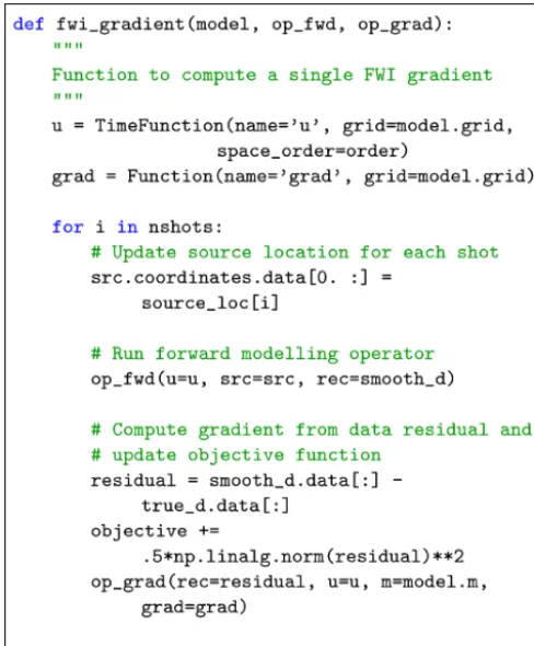
Figure 7.Definition of FWI gradient update.

shorthand expressionu.dt2. Combining the temporal and spatial derivative notations, and ignoring the source term q, we can now define the wave propagation component of Eq. (1) as a symbolic expression via Eq(m * u.dt2 - u.laplace, 0), where Eq is the SymPy represen-tation of an equation. In the resulting expression, all spa-tial and temporal derivatives are expanded using the cor-responding finite-difference terms. To define the propaga-tion of the wave in time, we can now rearrange the ex-pression to derive a stencil exex-pression for the forward sten-cil point in time, u(t+1t, x, y, z), denoted by the short-hand expression u.forward. The forward stencil corre-sponds to the explicit Euler time stepping that updates the next time stepu.forwardfrom the two previous ones u

andu.backward(Eq. 4). We use the SymPy utilitysolve

to automatically derive the explicit time-stepping scheme, as shown in Fig. 3 for the second order in space discretization.

u[t+1t, x, y, z] =2u[t, x, y, z] −u[t−1t, x, y, z]

+ 1t

2

m[x, y, z]1u[t, x, y, z]. (4)

The iteration over time to obtain the full solution is then generated by the Devito compiler from the time dimension information. Solving the wave equation with the above

ex-Figure 8.FWI algorithm with line search.

plicit Euler scheme is equivalent to a linear systemA(m)u= q_s, where the vectoruis the discrete wave field solution of the discrete wave equation,q_s is the source term, andA(m) is the matrix representation of the discrete wave equation. From Eq. (4) we can see that the matrixA(m)is a lower triangular matrix that reflects the time-marching structure of the stencil. Simulation of the wave field is equivalent to a forward substitution (solve row by row from the top) on the lower triangular matrixA(m). Since we do not consider complex valued PDEs, the adjoint ofA(m)is equivalent to its transpose denoted asA>_(m)_{and is an upper triangular}

matrix. The solution v of the discrete adjoint wave equa-tionA(m)>_v₌_q

afor an adjoint sourceqais equivalent to a backward substitution (solve from the bottom row to top row) on the upper triangular matrixA(m)>and is simulated backward in time starting from the last time step. These ma-trices are never explicitly formed, but are instead matrix-free operators with implicit implementation of the matrix–vector product,u=A(m)−1q_sas a forward stencil. The stencil for the adjoint wave equation in this self-adjoint case would sim-ply be obtained with solve(eqn, u.backward) and the compiler will detect the backward-in-time update. 3.2.3 Boundary conditions

(8)

fi-1172 M. Louboutin et al.: Devito: an embedded domain-specific language for finite differences

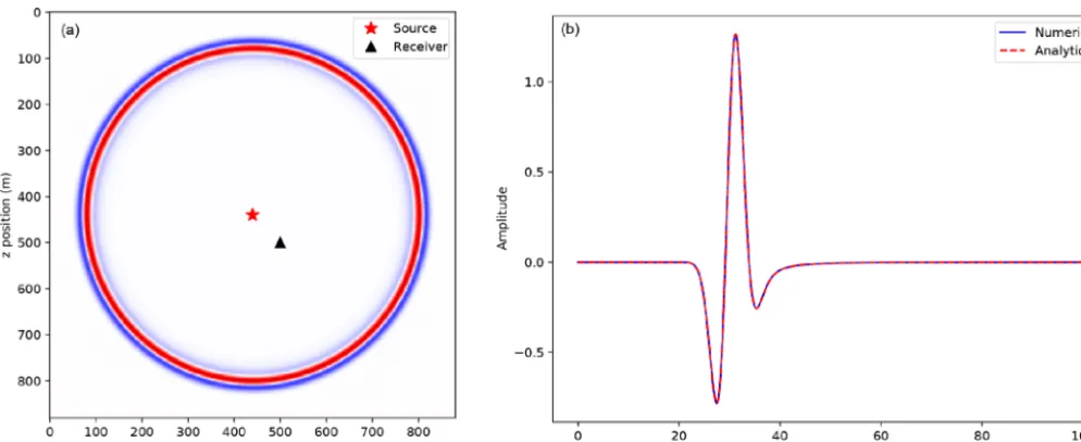
Figure 9.Numerical wave field for a constant velocity dt=0.1 ms,h=1 m and comparison with the analytical solution.

nite differences. In order to mimic an infinite domain, absorb-ing boundary conditions (ABCs) or perfectly matched layers (PMLs) are necessary (Clayton and Engquist, 1977). These two methods allow for the approximation of the wave field as it is in an infinite medium by damping and absorbing the waves within an extra layer at the limit of the domain to avoid unnatural reflections from the edge of the discrete domain.

The least computationally expensive method is the absorb-ing boundary condition that adds a sabsorb-ingle dampabsorb-ing mask in a finite layer around the physical domain. This absorbing con-dition can be included in the wave equation as

m[x, y, z]d

2_u_[_{t, x, y, z}_]

dt2 −1u[t, x, y, z]

+η[x, y, z]du[t, x, y, z]

dt =0. (5)

The η[x, y, z] parameter is equal to 0 inside the physi-cal domain and increasing from inside to outside within the damping layer. The dampening parameterηcan follow a lin-ear or exponential curve depending on the frequency band and width of the dampening layer. For methods based on more accurate modeling, for example in simulation-based ac-quisition design (Liu and Fomel, 2011; Wason et al., 2017; Naghizadeh and Sacchi, 2009; Kumar et al., 2015), a full im-plementation of the PML will be necessary to avoid weak reflections from the domain limits.

3.2.4 Sparse point interpolation

Seismic inversion relies on data-fitting algorithms, and hence we need to support sparse operations such as source injection and wave field (u[t, x, y, z]) measurement at arbitrary grid locations. Both operations occur at sparse domain points,

which do not necessarily align with the logical Cartesian grid used to compute the discrete solution u(t, x, y, z). Since such operations are not captured by the finite-difference ab-stractions for implementing PDEs, Devito implements a sec-ondary high-level representation of sparse objects (Lange et al., 2017) to create a set of SymPy expressions that per-form polynomial interpolation within the containing grid cell from predefined coefficient matrices.

The necessary expressions to perform interpolation and in-jection are automatically generated through a dedicated sym-bol type,SparseFunction, which associates a set of co-ordinates with the symbol representing a set of nonaligned points. For example, the syntaxp.interpolate(expr)

provided by aSparseFunction p will generate a sym-bolic expression that interpolates a generic expression

expr onto the sparse point locations defined byp, while

p.inject(field, expr)will evaluate and addexpr

to each enclosing point infield. The generated SymPy ex-pressions are passed to DevitoOperatorobjects alongside the main stencil expression to be incorporated into the gener-ated C kernel code. A complete setup of the acoustic wave equation with absorbing boundaries, injection of a source function, and measurement of wave fields via interpolation at receiver locations can be found in Sect. 4.2.

4 Seismic modeling and inversion

(9)

cap-M. Louboutin et al.: Devito: an embedded domain-specific language for finite differences 1173

Figure 10.Time discretization convergence analysis for a fixed grid, fixed propagation time (150 ms), and varying time step values. The result is plotted in a logarithmic scale and the numerical convergence rate (1.94 slope) shows that the numerical solution is accurate.

Figure 11.Comparison of the numerical convergence rate of the spatial finite-difference scheme with the theoretical convergence rate from the Taylor theory. The theoretical rates are the dotted line with the corresponding colors. The result is plotted in a logarithmic scale to highlight the convergence orders as linear slopes and the numerical convergence rates show that numerical solution is accurate.

tured by a set of hydrophones that can be classified as ei-ther moving receivers (cables dragged behind a source ves-sel) or static receivers (ocean bottom nodes or cables). From the acquired data, physical properties of the subsurface such as wave speed or density can be reconstructed by

minimiz-ing the misfit between the recorded measurements and the numerically modeled seismic data.

4.1 Full-waveform inversion

(10)

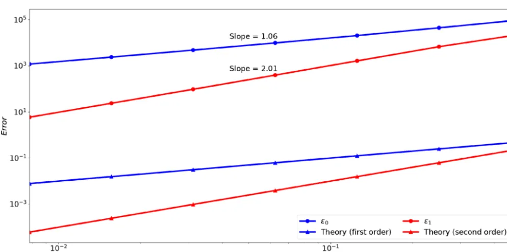
Figure 12.Gradient test for the acoustic propagator. The first-order (blue) and second-order (red) errors are displayed in logarithmic scales to highlight the slopes. The numerical convergence order (1.06 and 2.01) shows that we have a correct implementation of the FWI operators.

optimization problem called full-waveform inversion (FWI). The method aims at recovering an accurate model of the dis-crete wave velocity, c, or alternatively the square slowness of the wave, m= 1

c2 (not an overload), from a given set of measurements of the pressure wave field u. Lions (1971), Tarantola (1984), Virieux and Operto (2009), and Haber et al. (2012) show that this can be expressed as a PDE-constrained optimization problem. After elimination of the PDE con-straint, the reduced objective function is defined as

minimize

m 8s(m)=

1

2kPru−dk

2

2 with u=A(m) −1_PT

sqs, (6)

wherePris the sampling operator at the receiver locations, PT_s (T is the transpose or adjoint) is the injection operator at the source locations, A(m)is the operator representing the discretized wave-equation matrix,uis the discrete synthetic pressure wave field,q_sis the corresponding pressure source, anddis the measured data. While we consider the acoustic isotropic wave equation for simplicity here, in practice, mul-tiple implementations of the wave-equation operator A(m) are possible depending on the choice of physics. In the most advanced case,m would not only contain the square slow-ness but also anisotropic or orthorhombic parameters.

To solve this optimization problem with a gradient-based method, we use the adjoint-state method to evaluate the gra-dient (Plessix, 2006; Haber et al., 2012):

∇8s(m)= nt X

t=1

u[t]vt t[t] =JTδds, (7)

wherent is the number of computational time steps,δds= (Pru−d)is the data residual (difference between the mea-sured data and the modeled data),Jis the Jacobian operator, andv_{t t}is the second-order time derivative of the adjoint wave field that solves

AT(m)v=PT_rδds. (8)

The discretized adjoint system in Eq. (8) represents an up-per triangular matrix that is solvable by modeling wave prop-agation backwards in time (starting from the last time step). The adjoint-state method therefore requires a wave-equation solve for both the forward and adjoint wave fields to com-pute the gradient. An accurate and consistent adjoint model for the solution of the optimization problem is therefore of fundamental importance.

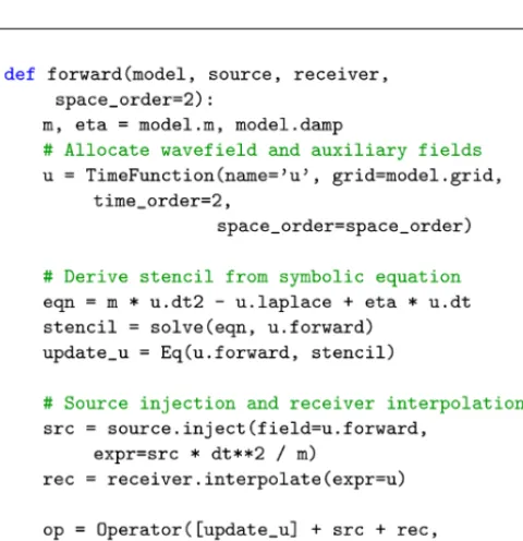
4.2 Acoustic forward modeling operator

(11)

Figure 13.FWI on the acoustic Marmousi-ii model. Panel(a)is the true velocity model, panel(b)is the initial velocity model, panel(c)is the inverted velocity at the last iteration of the iterative inversion, and panel(d)is the convergence.

locations. The shape of the computational domain is hereby provided by a utility objectmodel, while the damping term ηdu[x, y, z, t_dt ]is implemented via a utility symboletadefined as aFunctionobject. It is important to note that the dis-cretization order of the spatial derivatives is passed as an external parameter orderand carried as metadata by the wave field symbol uduring construction, allowing the user to freely change the underlying stencil order.

The main (PDE) stencil expression to update the state of the wave field is derived from the high-level wave-equation expression eqn = u.dt2 - u.laplace +

damp*u.dtusing SymPy utilities as demonstrated before in Fig. 3. Additional expressions for the injection of the wave source via the SparseFunction object src are then generated for the forward wave field, and the source time signature is discretized onto the computational grid via the symbolic expressionsrc * dt**2 / m. The weight dt2

(12)

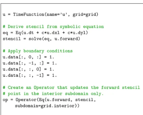
Figure 14. Convection equation in Devito. In this example, the initial Dirichlet boundary conditions are set to 1 using the API indexing feature, which allows us to assign values to the TensorFunctiondata.

The combined list of stencils, a sum in Python that adds the different expressions that update the wave field at the next time step, injects the source, interpolates at the receivers, and is then passed to theOperatorconstructor alongside a defi-nition of the spatial and temporal spacinghx, hy, hz, 1t pro-vided by themodelutility. Devito then transforms this list of stencil expressions into loops (inferred from the symbolic functions), replaces all necessary constants by their values if requested, prints the generated C code, and compiles it. The operator is finally callable in Python withop.apply().

A more detailed explanation of the seismic setup and pa-rameters such as the source and receiver terms in Fig. 4 is covered in Louboutin et al. (2017b).

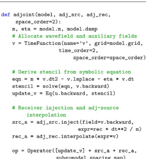
4.3 Discrete adjoint wave equation and FWI gradient

To create the adjoint that pairs with the above forward modeling propagator we can make use of the fact that the isotropic acoustic wave equation is self-adjoint. This means that for the implementation of the forward wave equation

eqn, shown in Fig. 5, only the sign of the damping term needs to be inverted, as the dampening time derivative has to be defined in the direction of propagation (_{∂n(t )}∂ ). For the PDE stencil, however, we now rearrange the stencil ex-pression to update the backward wave field from the two next time steps asv[t−1t, x, y, z] =f (v[t, x, y, z],v[t+ 1t, x, y, z]). Moreover, the role of the sparse point symbols has changed (Eq. 8) so that we now inject time-dependent data at the receiver locations (adj_src), while sampling the wave field at the original source location (adj_rec).

Based on the definition of the adjoint operator, we can now define a similar operator to update the gradient according to Eq. (7). As shown in Fig. 6, we can replace the expression

to sample the wave field at the original source location with an accumulative update of the gradient field gradvia the symbolic expressionEq(grad, grad - u * v.dt2). To compute the gradient, the forward wave field at each time step must be available, which leads to significant ory requirements. Many methods exist to tackle this mem-ory issue, but all come with their advantages and disadvan-tages. For instance, we implemented optimal checkpointing with the library Revolve (Griewank and Walther, 2000) in Devito to drastically reduce the memory cost by only saving a partial time history and recomputing the forward wave field when needed (Kukreja et al., 2018). The memory reduction comes at an extra computational cost as optimal checkpoint-ing requires log(nt)+2 extra PDE solves. Another method is boundary wave field reconstruction (McMechan, 1983; Mit-tet, 1994; Raknes and Weibull, 2016) that saves the wave field only at the boundary of the model, but still requires us to recompute the forward wave field during the back-propagation. This boundary method has a reduced memory cost but necessitates the computation of the forward wave field twice (one extra PDE solve), once to get the data and a second time from the boundary values to compute the gradi-ent.

4.4 FWI using Devito operators

At this point, we have a forward propagator to model syn-thetic data in Fig. 4, the adjoint propagator for Eq. (8), and the FWI gradient of Eq. (7) in Fig. 6. With these three op-erators, we show the implementation of the FWI objective and gradient with Devito in Fig. 8. With the forward and ad-joint and/or gradient operator defined for a given source, we only need to add a loop over all the source experiments and the reduction operation on the gradients (sum the gradient for each source experiment together). In practice, this loop over sources is where the main task-based or MPI-based par-allelization happens. The wave-equation propagator does use some parallelization with multithreading or domain decom-position, but that parallelism requires communication. The parallelism-over-source experiment is task based and does not require any communication between the separate tasks as the gradient for each source can be computed indepen-dently and reduced to obtain the full gradient. With the com-plete gradient summed over the source experiments, we date the model with a simple fixed step-length gradient up-date (Cauchy, 1847).

(13)

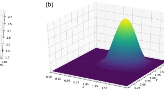
Figure 15.Initial(a)and final(b)time of the simulation of the convection equation.

Table 1.Adjoint test for different discretization orders in 2-D, com-puted on a two-layer model in double precision. The highlighted values represent the error in the values and indicate at which deci-mal the error appears.

Order <Fx,y> <x,FTy> Relative error 2nd order 7.9858×105 7.9858×105 0.0000×100 4th order 7.3044×105 7.3044×105 0.0000×100 6th order 7.2190×105 7.2190×105 4.8379×10−16 8th order 7.1960×105 7.1960×105 4.8534×10−16 10th order 7.1860×105 7.1860×105 3.2401×10−16 12th order 7.1804×105 7.1804×105 6.4852×10−16

Table 2.Adjoint test for different discretization orders in 3-D, com-puted on a two-layer model in double precision. The highlighted values indicate the error in the values and indicate at which decimal the error appears.

Order <Fx,y> <x,FTy> Relative error 2nd order 5.3840×104 5.3840×104 1.3514×10−16 4th order 4.4725×104 4.4725×104 3.2536×10−16 6th order 4.3097×104 4.3097×104 3.3766×10−16 8th order 4.2529×104 4.2529×104 3.4216×10−16 10th order 4.2254×104 4.2254×104 0.0000×100 12th order 4.2094×104 4.2094×104 1.7285×10−16

5 Verification

Given the operators defined in Sect. 3 we now verify the cor-rectness of the code generated by the Devito compiler. We first verify that the discretized wave equation satisfies the convergence properties defined by the order of discretization, and secondly we verify the correctness of the discrete adjoint and computed gradient.

5.1 Numerical accuracy

The numerical accuracies of the forward modeling operator (Fig. 4) and the runtime achieved for a given spatial dis-cretization order and grid size are compared to the analyti-cal solution of the wave equation in constant media. We de-fine two measures of the accuracy that compare the numer-ical wave field in constant velocity media to the analytnumer-ical solution:

– accuracy versus size, whereby we compare the obtained numerical accuracy as a function of the spatial sampling size (grid spacing); and

– accuracy versus time, whereby we compare the ob-tained numerical accuracy as a function of runtime for a given physical model (fixed shape in physical units, variable grid spacing).

The measure of accuracy of a numerical solution relies on a hypothesis that we satisfy for these two tests:

– the domain is large enough and the propagation time small enough to ignore boundary-related effects, i.e., the wave field never reaches the limits of the domain; and

– the source is located on the grid and is a discrete approx-imation of the Dirac to avoid spatial interpolation errors. This hypothesis guarantees the existence of the analyti-cal and numerianalyti-cal solution for any spatial discretization (Igel, 2016).

5.1.1 Convergence in time

(14)

Figure 16.Burgers’ equations in Devito. In this example, we ex-plicitly use the FD functionfirst_derivative. This function provides more flexibility and allows us to take an upwind derivative, rather than a standard centered derivative (x), to avoid odd–even coupling, which leads to chessboard artifacts in the solution.

at the center. We compare the numerical solution to the ana-lytical solution in Fig. 9.

The analytical solution is defined as (Watanabe, 2015)

us(r, t )= 1 2π

∞

Z

−∞

{−iπ H₀(2)(kr) q(ω)eiωtdω}, (9)

r= q

(x−xsrc)2+(y−ysrc)2, (10) whereH₀(2)is the Hankel function of second kind andq(ω)is the spectrum of the source function. As we can see in Fig. 10 the error decreases nearly quadratically with the size of the

time step with a time convergence rate slope of 1.94 in loga-rithmic scale that matches the theoretical expectation from a second-order temporal discretization.

5.1.2 Spatial discretization analysis

The spatial discretization analysis follows the same method as the temporal discretization analysis. We model a wave field for a fixed temporal setup with a small enough time step to ensure negligible time discretization error (dt=

0.00625 ms). We vary the grid spacing (dx) and spatial dis-cretization order and then compute the error between the numerical and analytical solution. The convergence rates should follow the theoretical rates defined in Eq. (2). In detail, for akth-order discretization in space, the error be-tween the numerical and analytical solution should decrease asO(dxk). The best way to look at the convergence results is to plot the error in logarithmic scale and verify that the error decreases linearly with slopek. We show the convergence re-sults in Fig. 11. The numerical convergence rates follow the theoretical ones for every tested orderk=2,4,6,8 with the exception of the 10th order for small grid size. This is mainly due to reaching the limits of the numerical accuracy and a value of the error on par with the temporal discretization er-ror. This behavior for high-order and small grids is, however, in accordance with the literature as in Wang et al. (2017).

The numerical slopes obtained and displayed in Fig. 11 demonstrate that the spatial finite difference follows the the-oretical errors and converges to the analytical solution at the expected rate. These two convergence results (time and space) verify the accuracy and correctness of the symbolic discretization with Devito. With this validated simulated wave field, we can now verify the implementation of the op-erators for inversion.

5.2 Propagators verification for inversion

We concentrate now on two tests, namely the adjoint test (or dot test) and the gradient test. The adjoint-state gradi-ent of the objective function defined in Eq. (7) relies on the solutions of the forward and adjoint wave equations; therefore, the first mandatory property to verify is the ex-act derivation of the discrete adjoint wave equation. The mathematical test we use is the standard adjoint property or dot test: for any random x∈span(PsA(m)−TP−rT),y∈ span(PrA(m)−1P−sT)

<PrA(m)−1P−sTx,y>−<x,PsA(m)−TP−rTy> <PrA(m)−1P−sTx,y>

=0.0. (11)

(15)

Figure 17.Initial(a)and final(b)time of the simulation of the Burgers’ equations.

of the adjoint operator for any order in both 2-D and 3-D. We observe that the discrete adjoint is accurate up to numerical precision for any order in 2-D and 3-D with an error of order 1×10−16. In combination with the previous numerical anal-ysis of the forward modeling propagator that guarantees that we solve the wave equation, this result verifies that the ad-joint propagator is the exact numerical adad-joint of the forward propagator and that it implements the adjoint wave equation. With the forward and adjoint propagators tested, we finally verify that the Devito operator that implements the gradient of the FWI objective function (Eq. 7, Fig. 6) is accurate with respect to the Taylor expansion of the FWI objective func-tion. For a given velocity model and associated squared slow-nessm, the Taylor expansion of the FWI objective function from Eq. (6) for a model perturbationdmand a perturbation scalehis

8s(m+hdm)=8s(m)+O(h)

8s(m+hdm)=8s(m)+hh∇8s(m),dmi +O(h2). (12) These two equations constitute the gradient test whereby we define a small model perturbationdmand vary the value of hbetween 10−6and 100and compute the error terms: 0=8s(m+hdm)−8s(m)

1=8s(m+hdm)−8s(m)−hh∇8s(m),dmi. (13) We plot the evolution of the error terms as a function of the perturbation scalehknowing0should be first order (linear with slope 1 in a logarithmic scale) and1should be second order (linear with slope 2 in a logarithmic scale). We exe-cuted the gradient test defined in Eq. (12) in double precision with an eighth-order spatial discretization. The test can be run for higher orders in the same manner but since it has al-ready been demonstrated that the adjoint is accurate for all orders, the same results would be obtained.

In Fig. 12, the matching slope of the error term with the theoreticalhandh2slopes from the Taylor expansion

veri-fies the accuracy of the inversion operators. With all the indi-vidual parts necessary for seismic inversion, we now validate our implementation in a simple but realistic example. 5.3 Validation: full-waveform inversion

We show a simple example of FWI in Eq. (7) on the Marmousi-ii model (Versteeg, 1994). This result was ob-tained with the Julia interface to Devito JUDI (Witte et al., 2018, 2019) that provides high-level abstraction for opti-mization and linear algebra. The model size is 4 km×16 km discretized with a 10 m grid in both directions. We use a 10 Hz Ricker wavelet with 4 s recording. The receivers are placed at the ocean bottom (210 m of depth) every 10 m. We invert for the velocity with all the sources, spaced by 50 m at 10 m of depth for a total of 300 sources. The inversion algorithm used is minConf_PQN (Schmidt et al., 2009), an l-BFGS algorithm with bound constraints (minimum and max-imum velocity value constraints). While conventional opti-mization would run the algorithm to convergence, this strat-egy is computationally not feasible for FWI. As each itera-tion requires two PDE solves per sourceqs(see adjoint state in Sect. 4), we can only affordO(10)iterations in practice (O(104)PDE solves in total). In this example, we fix the number of function evaluations to 20, which, with the line search, corresponds to 15 iterations. The result is shown in Fig. 13 and we can see that we obtain a good reconstruc-tion of the true model. More advanced algorithms and con-straints will be necessary for more complex problems such as a less accurate initial model, noisy data, or field-recorded data (Witte et al., 2018; Peters and Herrmann, 2017); how-ever, the wave propagator would not be impacted, making this example a good proof of concept for Devito.

(16)

Figure 18.Poisson equation in Devito with field swap in Python.

can implement all the required propagators and the FWI gra-dient in a few lines in a concise and mathematical manner. Second, as we obtained these results with JUDI (Witte et al., 2019), a seismic inversion framework that provides a high-level linear abstraction layer on top of Devito for seismic in-version, this example illustrates that Devito is fully compat-ible with external languages and optimization toolboxes and allows users to use our symbolic DSL for finite differences within their own inversion framework.

5.4 Computational fluid dynamics

Finally, we describe three classical computational fluid dy-namics examples to highlight the flexibility of Devito for an-other application domain. Additional CFD examples can be

Figure 19.Poisson equation in Devito with buffered dimension for automatic swap at each iteration.

found in the Devito code repository in the form of a set of Jupyter notebooks. The three examples we describe here are the convection equation, the Burgers’ equation, and the Pois-son equation. These examples are adapted from Barba and Forsyth (2018), and the example repository contains both the original Python implementation with NumPy and the imple-mentation with Devito for comparison.

5.4.1 Convection

The convection governing equation for a fielduand a speed cin two dimensions is

∂u ∂t +c

∂u ∂x+c

∂u

∂y =0. (14)

(17)

Figure 20.Right-hand side(a)and solution(b)of the Poisson equations.

Constantthat can accept any runtime value. We then dis-cretized the PDE using forward differences in time and back-ward differences in space:

un_{i, j}+1=un_{i, j}−c1t 1x(u

n i, j−u

n i−1, j)

−c1t 1y(u

n i, j−u

n

i, j−1), (15)

which is implemented in Devito as in Fig. 14.

The solution of the convection equation is displayed in Fig. 15 that shows the evolution of the fieldu, and the solu-tion is consistent with the expected result produced by Barba and Forsyth (2018).

5.4.2 Burgers’ equation

In this second example, we show the solution of the Burg-ers’ equation. This example demonstrates that Devito sup-ports coupled systems of equations and nonlinear equations easily. The Burgers’ equation in two dimensions is defined as the following coupled PDE system:

 

 ∂u ∂t +u

∂u ∂x+v

∂u ∂y =ν

∂2u ∂x2+

∂2u ∂y2

,

∂v ∂t +u

∂v ∂x+v

∂v ∂y =ν

∂2v ∂x2 +

∂2v ∂y2

, (16)

whereuandvare the two components of the solution and ν is the diffusion coefficient of the medium. The system of coupled equations is implemented in Devito in a few lines as shown in Fig. 16.

We show the initial state and the solution at the last time step of the Burgers’ equation in Fig. 17. Once again, the solution corresponds to the reference solution of Barba and Forsyth (2018).

5.4.3 Poisson

We finally show the implementation of a solver for the Pois-son equation in Devito. While the PoisPois-son equation is not time dependent, the solution is obtained with an iterative

solver and the simplest one can easily be implemented with finite differences. The Poisson equation for a fieldp and a right-hand sidebis defined as

∂2p ∂x2+

∂2p

∂y2 =b, (17)

and its solution can be computed iteratively with

pn_{i, j}+1=

(p_in+1, j+pni−1, j)1y2+(pi, jn +1+pni, j−1)1x2−bni, j1x21y2

2(1x2₊_1y2₎ , (18)

where the expression in Eq. (18) is computed until either the number of iterations is reached (our example case) or more realistically when ||p_{i, j}n+1−pn_{i, j}||< . We show two different implementations of a Poisson solver in Figs. 18 and 19. While these two implementations produce the same result, the second one takes advantage of Devito’s

BufferedDimension that allows us to iterate automat-ically alternating betweenpnandpn+1as the two different time buffers in theTimeFunction.

The solution of the Poisson equation is displayed in Fig. 20 with its right-hand sideb.

These examples demonstrate the flexibility of Devito and show that a broad range of PDEs can easily be implemented with Devito, including a nonlinear equation, a coupled PDE system, and steady-state problems.

6 Performance

(18)

Figure 21.Different spatial discretization order accuracies against runtime for a fixed physical setup (model size in m and propagation time).

6.1 Error–cost analysis

Devito’s automatic code generation lets users define the spa-tial and temporal order of FD stencils symbolically and with-out having to re-implement long stencils by hand. This al-lows users to experiment with trade-offs between discretiza-tion errors and runtime, as higher-order FD stencils provide more accurate solutions that come at increased runtime. For our error–cost analysis, we compare absolute error in L2 norm between the numerical and the reference solution to the time to solution (the numerical and reference solution are defined in Sect. 5). Figure 21 shows the runtime and numeri-cal error obtained for a fixed physinumeri-cal setup. We use the same parameter as in Sect. 5.1 with a domain of 400 m×400 m and we simulate the wave propagation for 150 ms.

The results in Fig. 21 illustrate that higher-order dis-cretizations produce a more accurate solution on a coarser grid with a shorter runtime. This result is very useful for in-verse problems, as a coarser grid requires less memory and fewer time steps. A grid size 2 times bigger implies a reduc-tion of memory usage by a factor of 24for 3-D modeling. Devito then allows users to design FD simulators for inver-sion in an optimal way, whereby the discretization order and grid size can be chosen according to the desired numerical accuracy and availability of computational resources. While a near-linear evolution of the runtime with increasing space order might be expected, we do not see such a behavior in practice. The main reason for this is that the effect of De-vito’s performance optimizations for different space orders is difficult to predict and does not necessarily follow a linear relationship. On top of these optimizations, the runtimes also

Figure 22.Roofline plots for a 512×512×512 model on a Skylake 8180 architecture. The runtimes correspond to 1000 ms of modeling for four different spatial discretization orders (4, 8, 12, 16).

include the source injection and receiver interpolation, which impact the runtime in a nonlinear way. Therefore, these re-sults are still acceptable. The order of the FD stencils also af-fects the best possible hardware usage that can theoretically be achieved and whether an algorithm is compute or memory bound, a trade-off that is described by the roofline model. 6.2 Roofline analysis

(19)

Figure 23.Roofline plots for a 768×768×768 model on a Skylake 8180 architecture. The runtimes correspond to 1000 ms of modeling for four different spatial discretization orders (4, 8, 12, 16).

Figure 24.Roofline plots for a 1024×1024×1024 model on a Sky-lake 8180 architecture. The runtimes correspond to 1000 ms of mod-eling for four different spatial discretization orders (4, 8, 12, 16).

a finite-difference scheme, this method provides an estimate of the best achievable performance on the underlying architecture, as well as an absolute measure of the hardware usage. We also show a more classical metric, namely time to solution, in addition to the roofline plots, as both are essential for a clear picture of the achieved performance. The experiments were run on an Intel Skylake 8180 ar-chitecture (28 physical cores, 38.5 MB shared L3 cache, with cores operating at 2.5 Ghz). The observed STREAM TRIAD (McCalpin, 1991–2007) was 105 GB s−1_{. The} maximum single-precision FLOP performance was calcu-lated as #cores·#avx units·#data items per vector register·

2(fused multiply-add)·core frequency=4480 GFLOPs s−1. A (more realistic) performance peak of 3285 GFLOPs s−1 was determined by running the LINPACK benchmark (Dongarra, 1988). These values are used to construct the roofline plots. In the performance results presented in this

section, the operational intensity (OI) is computed by the Devito profiler from the symbolic expression after the compiler optimization. While the theoretical OI could be used, we chose to recompute it from the final optimized symbolic stencil for a more accurate performance measure. A more detailed overview of Devito’s performance model is described in Luporini et al. (2018).

We show three different roofline plots, one plot for each domain size attempted, in Figs. 22, 23, and 24. Different space orders are represented as different data points. The time to solution in seconds is annotated next to each data point. The experiments were run with all performance opti-mizations enabled. Because auto-tuning is used at runtime to determine the optimal loop-blocking structure, timing only commences after auto-tuning has finished. The reported op-erational intensity benefits from the use of expression trans-formations, as described in Sect. 3; particularly relevant for this problem is the factorization of FD weights.

We observe that the time to solution increases nearly lin-early with the size of the domain. For example, for a 16th-order discretization, we have a 17.1 s runtime for a 512×

512×512 domain and a 162.6 s runtime for a 1024×1024×

1024 domain (a domain 8 times bigger and about 9 times slower). This is not surprising: the computation lies in the memory-bound regime and the working sets never fit in the L3 cache. We also note a drop in performance with a 16th-order discretization (relative to both the other space 16th-orders and the attainable peak), especially when using larger do-mains (Figs. 23 and 24). Our hypothesis, supported by pro-filing with Intel VTune (Intel Corporation, 2016), is that this is due to inefficient memory usage, in particular misaligned data accesses. Our plan to improve the performance in this regime consists of resorting to a specialized stencil optimizer such as YASK (see Sect. 7). These results show that we have a portable framework that achieves good performance on dif-ferent architectures. There is small room for improvements, as the machine peak is still relatively distant, but 50 %–60 % of the attainable peak is usually considered very good. Fi-nally, we remark that testing on new architectures will only require extensions to the Devito compiler, if any, while the application code remains unchanged.

7 Future work

(20)

Adding specialized back ends such as YASK – meaning that Devito can generate and compile YASK code, rather than pure C/C++ – is the key for long-term performance porta-bility, one of the goals that we are pursuing. Another mo-tivation is to enable large-scale computations and as many different types of PDEs as possible. In practice, this means that a staggered grid setup with half-node discretization and domain decomposition will be required. These two main re-quirements to extend the DSL to a broader community and to more applications are in full development and will be made available in future releases.

8 Conclusions

We have introduced a DSL for time–domain simulation for inversion and its application to a seismic inverse problem based on the finite-difference method. Using the Devito DSL, a highly optimized and parallel finite-difference solver can be implemented within just a few lines of Python code. Al-though the current application focuses on features required for seismic imaging applications, Devito can already be used in problems based on other equations; a series of CFD exam-ples is included in the code repository.

The code traditionally used to solve such problems is highly complex. The primary reason for this is that the com-plexity introduced by the mathematics is interleaved with the complexity introduced by the performance engineering of the code to make it useful for practical purposes. By in-troducing a separation of concerns, these aspects are pled and simplified. Devito successfully achieves this decou-pling while delivering good computational performance and maintaining generality, both of which shall continue to be improved in future versions.

Code availability. The asset https://doi.org/10.5281/zenodo.1038305 (Louboutin et al., 2017c) is the official DOI for the release of Devito 3.1.0. The source code, examples, and test script are avail-able on GitHub at https://github.com/opesci/devito (last access: 24 March 2019) and contain a README for installation. A more detailed overview of the project, with a list of publication and documentation for the software generated with Sphinx, is available at http://www.devitoproject.org/ (last access: 24 March 2019). To install Devito:

git clone -b v3.1.0

https://github.com/opesci/devito

cd devito

conda env create -f environment.yml

source activate devito

pip install -e .

Author contributions. MAL, MIL, NK, and FL designed and im-plemented the symbolic interface and Sympy extension in Devito.

MIL, FL, MAL, NK, and PV implemented the Devito compiler and the code generation framework.

NK and MAL implemented the checkpointing for Devito. FJH and GJG were the PIs for the project and provided design and application input so that Devito would be usable and scalable.

PAW, MAL, and MIL developed and implemented the examples presented in this paper.

Competing interests. The authors declare that they have no conflict of interest.

Acknowledgements. The development of Devito was primarily supported through the Imperial College London Intel Parallel Com-puting Centre. We would also like to acknowledge support from the SINBAD II project and support from the member organizations of the SINBAD Consortium as well as EPSRC grants EP/M011054/1 and EP/L000407/1.

Edited by: Simon Unterstrasser

Reviewed by: Jørgen Dokken and one anonymous referee

References

Alnæs, M. S., Logg, A., Ølgaard, K. B., Rognes, M. E., and Wells, G. N.: Unified Form Language: a domain-specific language for weak formulations of partial differential equations, ACM T. Math. Software, 40, 9, https://doi.org/10.1145/2566630, 2014. Andreolli, C., Thierry, P., Borges, L., Skinner, G., and Yount, C.:

Chapter 23 – Characterization and Optimization Methodology Applied to Stencil Computations, in: High Performance Paral-lelism Pearls, edited by: Reinders, J. and Jeffers, J., 377–396, Morgan Kaufmann, Boston, https://doi.org/10.1016/B978-0-12-802118-7.00023-6, 2015.

Arbona, A., Miñano, B., Rigo, A., Bona, C., Palenzuela, C., Ar-tigues, A., Bona-Casas, C., and Massó, J.: Simflowny 2: An up-graded platform for scientific modeling and simulation, arXiv preprint arXiv:1702.04715, Computer Physics Communications, 229, 170–181, 2017.

Asanovi´c, K., Bodik, R., Catanzaro, B. C., Gebis, J. J., Husbands, P., Keutzer, K., Patterson, D. A., Plishker, W. L., Shalf, J., Williams, S. W., and Yelick, K. A.: The landscape of parallel computing research: A view from berkeley, Tech. rep., Technical Report UCB/EECS-2006-183, EECS Department, University of Califor-nia, Berkeley, 2006.

Backus, J.: The history of Fortran I, II, and III, in: History of pro-gramming languages I, ACM SIGPLAN Notices, 13, 165–180, 1978.

Barba, L. A. and Forsyth, G. F.: CFD Python: the 12 steps to Navier-Stokes equations, Journal of Open Source Education, 9, 21, https://doi.org/10.21105/jose.00021, 2018.

(21)

Implemen-M. Louboutin et al.: Devito: an embedded domain-specific language for finite differences 1185

tation, PLDI 2008, 101–113, ACM, New York, NY, USA, https://doi.org/10.1145/1375581.1375595, 2008.

Cárdenas, A. F. and Karplus, W. J.: PDEL – a language for partial differential equations, Commun. ACM, 13, 184–191, 1970. Cauchy, A.-L.: Méthode générale pour la résolution des

sys-tèmes d’équations simultanées, Compte Rendu des Séances de L’Académie des Sciences XXV, Série A, 25, 536–538, 1847. Christen, M., Schenk, O., and Burkhart, H.: PATUS: A Code

Gen-eration and Autotuning Framework for Parallel Iterative Stencil Computations on Modern Microarchitectures, in: Proceedings of the 2011 IEEE International Parallel & Distributed Processing Symposium, IPDPS 2011, 676–687, IEEE Computer Society, Washington, DC, USA, https://doi.org/10.1109/IPDPS.2011.70, 2011.

Clayton, R. and Engquist, B.: Absorbing boundary conditions for acoustic and elastic wave equations, B. Seismol. Soc. Am., 67, 1529–1540, 1977.

Colella, P.: Defining Software Requirements for Scientific Comput-ing, DARPA HPCS, 2004.

Cook Jr., G. O.: ALPAL: A tool for the development of large-scale simulation codes, Tech. rep., Lawrence Livermore National Lab., CA, USA, 1988.

Dongarra, J.: The LINPACK Benchmark: An Explanation, in: Proceedings of the 1st International Conference on Super-computing, 456–474, Springer Verlag, London, UK, avail-able at: http://dl.acm.org/citation.cfm?id=647970.742568 (last access: 24 March 2019), 1988.

Farrell, P. E., Ham, D. A., Funke, S. W., and Rognes, M. E.: Au-tomated Derivation of the Adjoint of High-Level Transient Fi-nite Element Programs, SIAM J. Sci. Comput., 35, C369–C393, https://doi.org/10.1137/120873558, 2013.

Fomel, S., Sava, P., Vlad, I., Liu, Y., and Bashkardin, V.: Mada-gascar: open-source software project for multidimensional data analysis and reproducible computational experiments, Journal of Open Research Software, 1, p.e8, https://doi.org/10.5334/jors.ag, 2013.

Griewank, A. and Walther, A.: Algorithm 799: Revolve: An Im-plementation of Checkpointing for the Reverse or Adjoint Mode of Computational Differentiation, ACM Trans. Math. Softw., 26, 19–45, https://doi.org/10.1145/347837.347846, 2000.

Haber, E., Chung, M., and Herrmann, F. J.: An effective method for parameter estimation with PDE constraints with multiple right hand sides, SIAM J. Optimiz., 22, 739–757, https://doi.org/10.1137/11081126X, 2012.

Hawick, K. A. and Playne, D. P.: Simulation Software Genera-tion using a Domain-Specific Language for Partial Differential Field Equations, in: 11th International Conference on Software Engineering Research and Practice (SERP ’13), CSTN-187, p. SER3829, WorldComp, Las Vegas, USA, 2013.

Henretty, T., Veras, R., Franchetti, F., Pouchet, L.-N., Ramanu-jam, J., and Sadayappan, P.: A Stencil Compiler for Short-vector SIMD Architectures, in: Proceedings of the 27th Inter-national ACM Conference on InterInter-national Conference on Su-percomputing, ICS ’13, 13–24, ACM, New York, NY, USA, https://doi.org/10.1145/2464996.2467268, 2013.

Hopper, G. M.: The education of a computer, in: Proceedings of the 1952 ACM national meeting (Pittsburgh), 243–249, ACM, 1952. Igel, H.: Computational Seismology: A Practical In-troduction, Oxford University Press, 1. edn.,

avail-able at: https://global.oup.com/academic/product/ computational-seismology-9780198717409?cc=de&lang=en& (last access: 24 March 2019), 2016.

Intel Corporation: Intel VTune Performance Analyzer, avail-able at: https://software.intel.com/en-us/intel-vtune-amplifier-xe (last access: 24 March 2019), 2016.

Iverson, K. E.: A Programming Language, John Wiley & Sons, Inc., New York, NY, USA, 1962.

Jacobs, C. T., Jammy, S. P., and Sandham, N. D.: OpenSBLI: A framework for the automated derivation and parallel execution of finite difference solvers on a range of computer architectures, CoRR, abs/1609.01277, available at: http://arxiv.org/abs/1609. 01277 (last access: 24 March 2019), 2016.

Jones, J. L.: A survey of automatic coding techniques for digital computers, Ph.D. thesis, Massachusetts Institute of Technology, Boston, MA, USA, 1954.

Köster, M., Leißa, R., Hack, S., Membarth, R., and Slusallek, P.: Platform-Specific Optimization and Mapping of Stencil Codes through Refinement, in: Proceedings of the 1st International Workshop on High-Performance Stencil Computations, 21 Jan-uary 2014, Vienna, Austria, 1–6, 2014.

Kukreja, N., Hückelheim, J., Lange, M., Louboutin, M., Walther, A., Funke, S. W., and Gorman, G.: High-level python abstrac-tions for optimal checkpointing in inversion problems, arXiv preprint arXiv:1802.02474, 2018.

Kumar, R., Wason, H., and Herrmann, F. J.: Source separa-tion for simultaneous towed-streamer marine acquisisepara-tion – a compressed sensing approach, Geophysics, 80, WD73–WD88, https://doi.org/10.1190/geo2015-0108.1, 2015.

Lange, M., Kukreja, N., Luporini, F., Louboutin, M., Yount, C., Hückelheim, J., and Gorman, G. J.: Optimised finite difference computation from symbolic equations, in: Proceedings of the 16th Python in Science Conference (SciPy 2017), 10–16 July, Austin, Texas, edited by: Huff, K., Lippa, D., Niederhut, D., and Pacer, M., 89–96, 2017.

Lions, J. L.: Optimal control of systems governed by partial differ-ential equations, 1st edn., Springer Verlag, Berlin, Heidelberg, 1971.

Liu, Y. and Fomel, S.: Seismic data interpolation beyond aliasing using regularized nonstationary autoregression, Geophysics, 76, V69–V77, https://doi.org/10.1190/geo2010-0231.1, 2011. Logg, A., Mardal, K.-A., Wells, and Wells, G.: Automated

Solu-tion of Differential EquaSolu-tions by the Finite Element Method, The FEniCS Book, Springer, https://doi.org/10.1007/978-3-642-23099-8, 2012.

Louboutin, M., Lange, M., Herrmann, F. J., Kukreja, N., and Gor-man, G.: Performance prediction of finite-difference solvers for different computer architectures, Comput. Geosci., 105, 148– 157, https://doi.org/10.1016/j.cageo.2017.04.014, 2017a. Louboutin, M., Witte, P., Lange, M., Kukreja, N., Luporini, F.,

Gorman, G., and Herrmann, F. J.: Full-waveform inversion, Part 1: Forward modeling, The Leading Edge, 36, 1033–1036, https://doi.org/10.1190/tle36121033.1, 2017b.

Louboutin, M., Luporini, F., Lange, M., Kukreja, N., Pandolfo, V., Kazakas, P., Zhang, S., Gorman, G., Hueckelheim, J., Peng, P., Velesko, P., and McCormick, D.: opesci/devito: Devito-3.1, https://doi.org/10.5281/zenodo.1038305, 2017.