Journal of Hydraulic Structures J. Hydraul. Struct., 2016; 2(1):48-57 DOI: 10.22055/jhs.2016.12650
Slope Stability Analysis Using a Self-Adaptive Genetic
Algorithm
Amir H. Ayati1
Hossein M.V. Samani2
Ali Haghighi3
Abstract
This paper introduces a methodology for soil slope stability analysis based on optimization, limit equilibrium principles and method of slices. In this study, the slope stability analysis problem is transformed into a constrained nonlinear optimization problem. To solve that, a Self-Adaptive Genetic Algorithm (GA) is utilized. In this study, the slope stability safety factors are the objective functions, slip surface parameters are the decision variables and, the equilibrium equations are the problem constraints. The proposed model satisfies all conditions of the equilibrium completely. It is also applicable to problems with different soil layers, variable soil properties and including pore water pressure. The model is applied against a benchmark example and the results are compared with previous studies. Accordingly, it is found computationally efficient and reliable.
Keywords: Slope stability analysis, self-adaptive GA, Method of slices, Equilibrium analysis, Safety factor
Received: 13 January 2016; Accepted: 18 July 2016
1. Introduction
Slope stability analysis is of geotechnical engineering problems that has received considerable attention from researchers worldwide. Equilibrium analyses of slope stability are widely used in design of excavation and embankment slopes. There exist a lot of successful applications and experiences on the limit equilibrium methods which make it very popular
1Civil Engineering Department, Faculty of Engineering, Shahid Chamran University of Ahvaz, Ahvaz, Iran, Email: [email protected] (Corresponding author)
2Civil Engineering Department, Faculty of Engineering, Shahid Chamran University of Ahvaz, Ahvaz, Iran
through their simplicity to implement and accuracy of results as well. Indeed, the limit equilibrium methods have been the most widely used methods for slope stability analysis [1]. These methods, in general, satisfy the force and moment equilibrium; boundary conditions and the failure criterion along the slip surface. In context of the limit equilibrium methods, methods of slices are extensively used to cope with complex slope geometries, variable soil properties and the existence of pore water pressure.
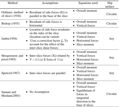
Reviewing the literature, the slope stability methods can be categorized in two major groups consisting of the numerical methods, mostly the finite element method [2-4] and analytical methods, mostly based on the methods of slices. The latter encompasses; the ordinary method (1936) [5], simplified Bishop method (1955) [6], simplified Janbu method (1956) [7], Corps of Engineers method (1967) [8], Spencer method (1967) [9], Morgenstern-Price method (1965) [10], Samani and Meidani (2003) [11]. These methods are somehow different in defining the safety factor equations. They also use different assumptions to derive the governing equations and carrying out the stability analyzes as summarized in Table 1.
There are two kinds of solutions for the problem. The first is a simplified solution where the
Table 1. Different methods of slices for slope stability analysis
Method Assumptions Equations used Slip
surface
Ordinary method of slices (1936)
Resultant of side forces (Ei) is parallel to the base of the slice
Overall moment
Circular
Bishop (1955) Resultant of side forces is horizontal
Overall moment
Vertical forces Circular
Janbu(1956)
Location of side force resultants on the sides of the slice
(location can be varied) Uses a correction factor 𝑓𝑜 To
account for the effect of the inter-slice shear forces.
Overall moment Vertical forces Horizontal forces Slice moment
Any
Morgenstern and price(1965)
Inter-slice forces (Xi) related by V = 𝜆 f (x) E form of f (x)
Overall moment Vertical forces Horizontal forces Slice moment
Any
Spencer(1967) Inter-slice forces are parallel
Overall moment Vertical forces Horizontal forces Slice moment
Any
Samani and Meidani(2003)
No Assumption
Overall moment Vertical forces Equilibrium of
forces in tangential direction to the base of slices
conditions of static equilibrium are not rigorously satisfied. In this solution, some assumptions are made to obtain the solution in a simple form. The second is a rigorous solution where the equilibrium conditions are completely satisfied [12].
In general, the main features of limit equilibrium methods can be summarized as the following [13]:
1) The sliding body above an assumed slip surface is divided into a number of vertical (or inclined) slices.
2) The strength of the slip surface is mobilized by the same factor of safety, where the cohesion component and the friction component of the strength are reduced equally.
3) Assumptions regarding inter-slice forces are employed to render the problem determinate. 4) The factor of safety is derived from the force or/and moment equilibrium equations.
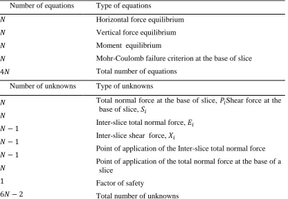
Table 2. Summary of equations and unknowns associated with limit equilibrium methods Number of equations Type of equations
𝑁
𝑁 𝑁 𝑁
4𝑁
Horizontal force equilibrium
Vertical force equilibrium
Moment equilibrium
Mohr-Coulomb failure criterion at the base of slice
Total number of equations
Number of unknowns Type of unknowns
𝑁 𝑁
𝑁 − 1 𝑁 − 1 𝑁 − 1
𝑁 1 6𝑁 − 2
Total normal force at the base of slice, 𝑃𝑖Shear force at the base of slice, 𝑆𝑖
Inter-slice total normal force, 𝐸𝑖
Inter-slice shear force, 𝑋𝑖
Point of application of the Inter-slice total normal force
Point of application of the total normal force at the base of a slice
Factor of safety
Total number of unknowns
Note: N is the number of slices, 𝑃𝑖, 𝑆𝑖, 𝐸𝑖, 𝑋𝑖 are introduced in figure 2.
introduces a self-adaptive GA to solve the system of equations of slope stability analysis. The applied procedure satisfies all conditions of equilibrium with a high degree of precision. Using the self-adaptive GA, all constraints of the problem are automatically handled into the optimization with no need for any penalty function on the objective function. For this purpose, a slope stability analyzer model is developed and coupled to the GA. The proposed model is applied against a benchmark example and the results are compared with the other conventional methods.
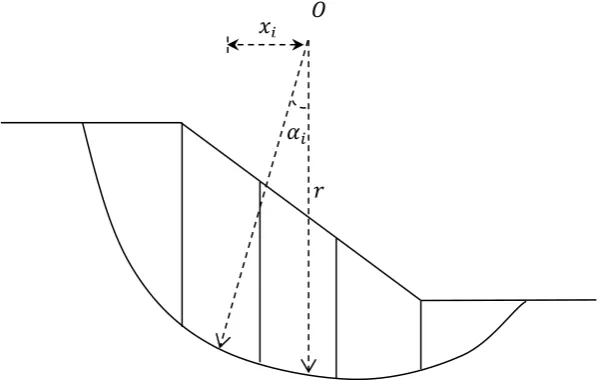
Figure 1. Sliding circular surface subdivided into vertical slices
𝑙𝑖 𝑆𝑖
𝛼𝑖
𝑋𝑖 𝑍𝑖
Pi
𝑋𝑖+1
𝑍𝑖+1
𝑊𝑖
𝐸𝑖+1
𝐸𝑖
𝑥𝑖
𝛼𝑖
Figure 2. Free body diagram of a slice
2.
Governing EquationsGeotechnical engineers frequently use the limit equilibrium methods of analysis when studying slope stability problems. For this purpose, the methods of slices are the most commonly used technique for the sake of their easiness in concept and implementation as well as ability to accommodate complex geometrics and variable soil and water pressure conditions [14].
Fig. 1 shows the potential sliding mass along a trial slip surface through a homogenous slope. The sliding mass is subdivided into a number of vertical slices. The free body diagram of a slice is illustrated in Fig. 2. The forces acting on the slice are its own weight 𝑊𝑖 , slide forces, both having shear component 𝑋𝑖, and normal component 𝐸𝑖, and shear resistance 𝑆𝑖 and the normal force 𝑃𝑖 acting on the base of slice. Equating the moment of weight of the sliding mass with the moment of external forces acting on the slip surface about the center O of the slip circular surface yields:
∑ 𝑊𝑖 . 𝑥𝑖 = ∑ 𝑆𝑖 . 𝑟 (1)
where Wi is slice weight, Si is shear forces in tangential direction to the base of the slice, and xi and r are shown in Fig. 1. The relation between the shear strength of failure and equilibrium shear stress along the slide surface can be expressed as the following:
𝜏 =𝜏𝐹𝑓 (2) in which, F is the factor of safety and τf is the soil shear strength of failure calculated based on the Mohr-Clumb equation:
𝜏𝑓 = 𝐶′+ (
𝑃𝑖
𝑙𝑖− 𝑢𝑖) . tan 𝜙
′ (3)
where C′is drained cohesion of the soil, ϕ′is drained internal friction angle, l
i is the slice base length and ui is the pore water pressure.
Combining equation 2 and 3 gives:
τ =1
𝐹[𝐶 ′+ (𝑃𝑖
𝑙𝑖 − 𝑢𝑖) . 𝑡𝑎𝑛 𝜙
′] (4)
The vertical equilibrium for the slice i gives:
Wi+ Xi− Xi+1= Pi . cosαi+ Si . sinαi (5)
Rearranging for Pi yields:
Pi= (Wi+ Xi− Xi+1) . secαi− Si . tanαi (6)
Substituting the last expression in equation 4 and simplifying the result gives:
Si=
1
F+tanαi .tanϕ′{C
′. l
i+ [(Wi+ Xi− Xi+1). secαi− ui . li]. tan ϕ′} (7)
r. ∑{C′.li+[(Wi+Xi−Xi+1).secαi−ui .li].tan ϕ′}
F+tanαi .tanϕ′ = ∑ r. Wi. sinαi (8)
The summation of the normal inter-slice forces should also be zero:
∑(Ei− Ei+1) = 0 (9)
Resolving the force acting on the slice in a tangential direction to the base of the slice results:
Si= (Ei− Ei+1). cos αi+ (Wi+ Xi− Xi+1). secαi (10)
Therefor:
∑(Ei− Ei+1) = ∑[Si. sec αi+ (Wi+ Xi− Xi+1). tanαi] (11)
Insertion of the value of Si from equation 7 into equation 11 yields:
∑{ C′.li+[(Wi+Xi−Xi+1).secαi−ui .li].tan ϕ′
F+tanαi .tanϕ′ . secαi− (Wi+ Xi− Xi+1). tanαi} = 0 (12)
Equations 8 and 12 are respectively the moment and force equilibrium equations. These equations should be solved to determine the unknowns Xi for every slice and the factor of safety F.
3. The optimization problem
The analysis of slope stability using the limit equilibrium methods is performed in two steps: First, the calculation of the factor of safety for a given slip surface and, second, a search for the critical slip surface with the minimum factor of safety of the slope. As earlier mentioned, the number of equations is less than the number of unknowns and the system of equations is thus indeterminate. Since, the process of finding the critical slip surface is linked to a technique for finding the minimum factor of safety; it could be possible to consider the process as an optimization problem. Here, equation 13 is considered as the optimization objective function. The acceptable bounds for the problem decision variables Xi, xc, yc, and r are considered as the problem constraints on the objective function. By minimizing the objective function subjected to the following inequality constraints, optimum values of the aforementioned decision variables are obtained.
Minimize F (safety factor) Subject to: (13)
Xi_l≤ Xi≤ Xi_u i = 1,2, … , N
xc_l≤ xc≤ xc_u
yc_l≤ yc≤ yc_u
rl≤ r ≤ ru
(Eq. 8)2+(Eq. 12)2≤ ε (14)
4. Self-Adaptive GA
To solve the above constrained mathematical programming model, a self-adaptive GA is developed as the following on the basis of a standard real GA:
1- An initial population with NP chromosomes is randomly generated within range [0, 1]. The chromosomes are decoded based on the upper and lower bounds of decision variables. Accordingly, each chromosome contains a set of feasible shear components (𝑋𝑖) as well as the geometric parameters of slip surface (xc, yc, r). The slope stability analyzer program is run against each chromosome and the corresponding objective function (𝐹) and the violation (𝑉) of last constraint equation 14 are evaluated.
2- The binary tournament selection method [15] is used to select the parents. Through this step, the problem constraint (equation 14) is also handled so that, for each parent, two chromosomes x and y are randomly picked up from the population. 𝑥 wins the tournament if one of the following conditions is met otherwise, 𝑦 wins.
a. Both x and y are feasible but x has a greater objective function value. b. Both x and y are infeasible but x has a smaller constraint violation. c. x is feasible but y is not.
Accordingly, there is no need to penalize the objective function when a chromosome is infeasible. By using the above simple scheme, the GA can freely search into the problem decision space and gradually approach to the feasible regions.
The number of parents is considered to be half of the population size (NP/2). After all the required parents were selected, they are transferred to the mating pool to generate new offsprings.
3- The blend crossover method (BLX- α) proposed by Eshelman and Shaffer (1993) [16], is applied to each couple in the mating pool resulting in two children. When the crossover operator is applied to all couples, the population of children with NP size is created.
4- A few genes in the new population are mutated.
5- The children population is introduced to the slope stability analyzer program and F and
V values in each new chromosome are evaluated.
6- The old and new populations are combined resulting in a population with 2NP size. The combined population is then divided into two subsets with respect to the feasibility and infeasibility of the chromosomes. The chromosomes with zero constraint violation are transferred to the feasible subset and the chromosomes with nonzero constraint violation are transferred to the infeasible subset. Let the size of feasible and infeasible subsets be respectively NF and NI so that, NF + NI = 2NP.
7- To form the new generation, we need to select the best NP chromosomes from 2NP
in each generation and the next generation is derived from both, the elitism is automatically preserved in the GA.
8- After the new generation was formed, the algorithm is repeated from step 2 until no further improvement is seen in the objective function.
5. Example
In this section, an illustrative example from the literature is adopted and analyzed using the proposed method. The geometry and soil parameters are presented in Fig 3. It is supposed that the center of the coordinate system is at point A. The factor of safety and slip surface geometric parameters are considered to be unknown.
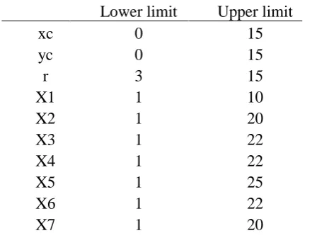
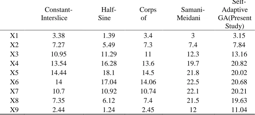
The example is solved with 10 slices. Upper and lower bounds of decision variables are shown in Table 3. To solve the problem the GA population was decided 50 and the mutation ratio is 0.05. After about 200 generations the best results of the optimization were obtained as the following; 𝐹 = 2.35; 𝑥𝑐 = 4.17 𝑚; 𝑦𝑐 = 11.67 𝑚 and 𝑟 = 9.4 𝑚. For more investigations, the safety factors evaluated study in Table 4. Also, Table 5 in the previous studies are compared to the current presents the inter-slice shear forces obtained here it is compared to the previous works. Accordingly, concluded that the model has a good agreement with the previous well-known methods. Furthermore, the maximum constraint violation of (𝐸𝑞8)2+(𝐸𝑞12)2 is obtained 7E-06 which means that, both moment and force equilibrium equations have been precisely fulfilled through the applied model.
Figure 3. Geometry and soil parameters of example
Table 3. Upper and lower bounds of unknown values
Lower limit Upper limit
xc 0 15
yc 0 15
r 3 15
X1 1 10
X2 1 20
X3 1 22
X4 1 22
X5 1 25
X6 1 22
X7 1 20
𝐴 𝑦
𝑥 3
1 𝛾𝑑
= 18 𝐾𝑁/𝑚3
𝐶′
= 12 𝐾𝑃𝑎
∅′ = 10°
X8 1 20
X9 1 10
Table 4. Factor of safety calculated by various methods
Bish op (1955)
Janb u (1956)
Morgenstern-Price (1965)
Samani-Meidani (2003)
Self-Adaptive GA (Present
study) 2.39
4
2.12
5 2.391 2.437 2.350
Table 5. Inter-slice shear force calculated by different methods
Constant-Interslice
Half-Sine
Corps of
Samani-Meidani
Self-Adaptive GA(Present
Study)
X1 3.38 1.39 3.4 3 3.15
X2 7.27 5.49 7.3 7.4 7.84
X3 10.95 11.29 11 12.3 13.16
X4 13.54 16.28 13.6 19.7 20.82
X5 14.44 18.1 14.5 21.8 20.02
X6 14 17.04 14.06 22.5 20.68
X7 10.7 10.92 10.74 22.1 20.21
X8 7.35 6.12 7.4 21.5 19.63
X9 2.44 1.24 2.45 12 11.04
6. Conclusion
References
1. Duncan, J. M. 1996, "State of the art: Limit equilibrium and finite-element analysis of slopes", Journal of Geotechnical Engineering, vol. 122, no. 7, pp. 577-596.
2. Griffiths, D.V. and Lane, P.A., 1999. Slope stability analysis by finite elements. Geotechnique, 49(3), pp.387-403.
3. Griffiths, D.V. and Fenton, G.A., 2004. Probabilistic slope stability analysis by finite elements. Journal of Geotechnical and Geoenvironmental Engineering, 130(5), pp.507-518.
4. Griffiths, D.V. and Marquez, R.M., 2007. Three-dimensional slope stability analysis by elasto-plastic finite elements. Geotechnique, 57(6), pp.537-546
5. Fellenius, W. 1936, "Calculation of the stability of earth dams", Transactions, 2nd Congress on Large Dams, Washington, pp. 445-462.
6. Bishop, A. W. 1955, "The use of the slip circle in the stability analysis of slopes", Geotechnique,vol. 5, no. 1, pp. 7-17.
7. Janbu, N., Bjerrum, L., & Kjaernsli, B. 1956, "Soil mechanics applied to some
engineering problems", Norwegian Geotechnical Institute Publication, vol. 16, pp. 1-93. 8. U.S.Army Corps of Engineers 1967, Stability of slopes and foundations, Engineering
manual,Vicksburg, Miss. Whitman, R.V., and Bailey, W.A.
9. Spencer, E. 1967, "Method of analysis of stability of embankments assuming parallel inter-slice forces", Geotechnique, vol. 17, no. 1, pp. 11-26.
10. Morgenstern, N. R. & Price, V. E. 1965, "Analysis of stability of general slip surfaces",Geotechnique, vol. 15, no. 1, pp. 79-93.
11. Samani, Hossein M. V., and Meidani, M. (2003). “Slope Stability Analysis Using A Non-linear Optimization Technique.” International Journal of Engineering, Vol. 16, No. 2. pp. 147-156.
12. Sarma, S. K. 1979, "Stability analysis of embankments and slopes", American Society of Civil Engineers, Journal of the Geotechnical Engineering Division, vol. 105, no. 12, pp. 1511-1524.
13. Zhu, D. Y., Lee, C. F., & Jiang, H. D. 2003, "Generalized framework of limit
equilibrium methods for slope stability analysis", Geotechnique, vol. 53, no. 4, pp. 377-395.
14. Terzaghi. K. and Peck. R. B. 1967.S oil mechanics i n engineering practice. (2nd ed.), John Wiley and Sons lnc. New York. N.Y.Deb,
15. K.,Pratap,A.,Agarwal.,S.,Meyarivan,T.,2002.A fast and elitist multi-objective genetic algorithm:NSGA-II.IEEETrans.Evolut.Comput. 6(2), 182–197.