Distributional Semantics Meets Multi-Label Learning

The Thirty-Third AAAI Conference on Artificial Intelligence (AAAI-19)

Distributional Semantics Meets Multi-Label Learning

Vivek Gupta,

_{Rahul Wadbude,}

_{Nagarajan Natarajan,}

Harish Karnick,

_{Prateek Jain,}

_{Piyush Rai}

1_{School of Computing, University of Utah,}2_{Computer Science Department, IIT Kanpur} 3_{Microsoft Research Lab, Bangalore}

[email protected], [email protected], [email protected], [email protected] [email protected], [email protected]

Abstract

We present a label embedding based approach to large-scale multi-label learning, drawing inspiration from ideas rooted in distributional semantics, specifically the Skip Gram Nega-tive Sampling (SGNS) approach, widely used to learn word embeddings. Besides leading to a highly scalable model for multi-label learning, our approach highlights interesting con-nections between label embedding methods commonly used for multi-label learning and paragraph embedding methods commonly used for learning representations of text data. The framework easily extends to incorporating auxiliary informa-tion such as label-label correlainforma-tions; this is crucial especially when many training instances are only partially annotated. To facilitate end-to-end learning, we develop a joint learning al-gorithm that can learn the embeddings as well as a regression model that predicts these embeddings for the new input to be annotated, via efficient gradient based methods. We demon-strate the effectiveness of our approach through an extensive set of experiments on a variety of benchmark datasets, and show that the proposed models perform favorably as compared to state-of-the-art methods for large-scale multi-label learning.

Introduction

Data generated in various domains are increasingly multi-labelin nature; images (e.g.Instagram) and documents (e.g.

Wikipedia) are often identified with multiple tags, online ad-vertisers often associate multiple search keywords with ads, and so on. Multi-label learning is the problem of learning to

annotateeach instance using a subset of labels from a po-tentially very large label vocabulary. Nowadays, multi-label learning problems can even have label vocabulary consisting of millions of labels, popularly known as extreme multi-label learning (Jain, Prabhu, and Varma 2016; Bhatia et al. 2015; Babbar and Sch¨olkopf 2017; Prabhu and Varma 2014).

The key challenges in multi-label learning, especially ex-treme multi-label learning, include: a) training instances may have a large fraction of labels missing, and b) the la-bels are often heavy-tailed (Bhatia et al. 2015; Jain, Prabhu, and Varma 2016) and predicting labels in the tail becomes significantly hard due to the lack of training data. For these reasons, and the sheer scale of data, traditional multi-label classifiers are rendered impractical. State-of-the-art ap-proaches to extreme multi-label learning fall broadly under

Copyright c2019, Association for the Advancement of Artificial Intelligence (www.aaai.org). All rights reserved.

two classes: 1) embedding based methods, e.g., LEML(Yu et al. 2014), WSABIE(Weston, Bengio, and Usunier 2010), SLEEC (Bhatia et al. 2015), PD-SPARSE (Yen et al. 2016), PPDSPARSE (Yen et al. 2017), and 2) tree-based meth-ods, e.g., FASTXML (Prabhu and Varma 2014) , PFAS

-TREXML (Jain, Prabhu, and Varma 2016), LEM (Tagami 2017b). The first class of approaches are generally scal-able and work by embedding the high-dimensional label vectors to a lower-dimensional space and learning a regres-sor in that space. In most cases, these methods rely on a key assumption that the binary label matrix is low rank and consequently the label vectors can be embedded into a lower-dimensional space. At the time of prediction, a de-compression matrix is used to retrieve the original label vector from the low-dimensional embeddings. As corrob-orated by recent empirical evidence (Bhatia et al. 2015; Jain, Prabhu, and Varma 2016), approaches based on stan-dard structural assumptions such as low-rank label matrix fail and perform poorly on the tail. The second class of meth-ods (tree-based) for multi-label learning try to move away from rigid structural assumptions (Prabhu and Varma 2014; Jain, Prabhu, and Varma 2016), and have been demonstrated to work very well especially on the tail labels.

distributional semantics approaches (Mikolov et al. 2013; Le and Mikolov 2014), widely used for learning non-linear representations of text data for NLP tasks, such as understand-ing word and document semantics, classifyunderstand-ing documents, etc. In future, we can try to generalize the method with other NLP techniques used for representing text documents such as LSTMs (Hochreiter and Schmidhuber 1997), RNNs (Jain and Medsker 1999) and skip-thought vector (Kiros et al. 2015) for embedding instance label vector. Our main contributions are summarized below.

1. We establish a connection between multi-label learning us-ing label embeddus-ing methods and the problem of learnus-ing distributional semantics in text data analysis. We leverage this connection to design a novel objective function for multi-label learning that can be solved efficiently using matrix factorization.

2. Unlike most existing multi-label learning methods, our method easily extends to leverage label co-occurrence information while learning the embeddings; this is espe-cially appealing when many training instances might have incomplete annotations.

3. Our models have much faster training times as compared to state-of-art label embedding methods for extreme multi-label learning, while being competitive in terms of la-bel prediction accuracies. We demonstrate this on several moderate-sized as well as very large-scale multi-label benchmark datasets.

4. We show improvement in performance by joint learning of embedding and regressors through a novel objective. Our jointly optimized objective is competitive with re-spect to state-of-the-art methods like ANNEXML (Tagami

2017a), DISMEC (Babbar and Sch¨olkopf 2017) and PPDSPARSE (Yen et al. 2017).

5. Our joint objective is flexible to incorporate online param-eter update using online stochastic gradient decent update algorithms. This can even help us in learning with limited labeled data. However, this is beyond the scope of this paper and is left as future work.

Problem Formulation and Background

We assume that we are given a set of training instances, e.g., documents in BoW/tf-idf representation,{x1,x2, . . . ,xn},

where xi ∈ Rd and the associated label/tag vectors {y₁,y₂, . . . ,y_n}, wherey_i ∈ {0,1}L_{. In many cases, one}

does not usually observe irrelevant labels; here yij = 1

indicates that the jth label is relevant for instance i but yij = 0 indicates that the label is missingor irrelevant.

LetY ∈ {0,1}n×L _{denote the matrix of label vectors. In}

addition, we may have access to label-label co-occurrence information, denoted byC∈_ZL×L₊ (e.g., number of times a pair of labels co-occur in some external source such as the wikipedia corpus). The goal in multi-label learning is to learn a vector-valued functionf : x 7→s, wheres ∈RL scores the labels (which can be used torankthe labels according to their relevance).

Embedding-based approaches typically modelfas a com-posite functionh(g(x))where,g:Rd→Rd

0

andh:Rd

0

→

RL. For example, assuming bothgandhas linear transfor-mations, one obtains the formulation proposed by (Yu et al. 2014). The functionsgandhcan be learnt using training instances or label vectors, or both. More recently, non-linear embedding methods have been shown to help improve multi-label prediction accuracies significantly. In this work, we follow the framework of (Bhatia et al. 2015), wheregis a linear transformation, buthis non-linear, and in particular, based onk-nearest neighbors in the embedded feature space.

In SLEEC, the functiong:_Rd_→

Rd

0

is given byg(x) =

VxwhereV ∈Rd

0

×d_{. The functionh:}

Rd

0

→RLis defined as:

h

z;{zi,yi} n i=1

= 1

|Nk| X

i∈Nk

y_i, (1)

wherezi=g(xi)andNkdenotes thek−nearest neighbor

training instances ofzin the embedded space. Our algorithm for predicting the labels of a new instance is identical to that of SLEECand is presented for convenience in Algorithm 1.

Note that, for speeding up predictions, the algorithm relies on clustering the training instancesxi; for each cluster of

instancesQτ, a different linear embeddinggτ, denoted by Vτ_{, is learnt.}

Algorithm 1Prediction Algorithm

Input: Test point: x, no. of nearest neighborsk, no. of desired labelsp.

1.Qτ: partition closest tox.

2.z←Vτ_x.

3. Nk ← k nearest neighbors ofzin the embedded

in-stances ofQτ.

4.s=h(z;{zi,yi}i∈Qτ)wherehis defined in 1

returntoppscoring labels according tos.

In this work, we focus on learning algorithms for the functions g and h, inspired by their successes in natural language processing in the context of learn-ing distributional semantics (Mikolov et al. 2013; Levy and Goldberg 2014). In particular, we use tech-niques for inferring word-vector embeddings for learning the function h using a) training label vectors y_i, and b) label-label correlationsC∈RL×L.

Word embeddings are desired in natural language process-ing in order to understand semantic relationships between words, also classifying text documents, etc. Given a text cor-pus consisting of a collection of documents, the goal is to embed each word in some space such that words appearing in similarcontexts(i.e. adjacent words in documents) should becloserin the space, than those that do not. In particular, we use theword2vecembedding approach (Mikolov et al. 2013) to learn an embedding of instances, using their label vectorsy₁,y₂, . . . ,y_n. SLEECalso uses nearest neighbors in the space of label vectorsy_iin order to learn the embed-dings. However, we show in experiments thatword2vec

missing labels. In the subsequent section, we discuss our al-gorithms for learning the embeddings and the training phase of multi-label learning.

Learning Instance and Label Embeddings

There are multiple algorithms in the literature for learning word embeddings (Mikolov et al. 2013; Pennington, Socher, and Manning 2014). In this work, we use the Skip Gram Negative Sampling (SGNS) technique, for two reasons a) it is shown to be competitive in natural language processing tasks, and more importantly, b) it presents a unique advantage in terms of scalability, which we will address shortly after discussing the technique.

Skip Gram Negative Sampling.In SGNS, the goal is to learn an embeddingz∈Rd

0

for each wordwin the vocabu-lary. To do so, words are considered in thecontextsin which they occur; contextcis typically defined as a fixed size win-dow of words around an occurrence of the word. The goal is to learnzsuch that the words in similar contexts are closer to each other in the embedded space. Letw0 ∈cdenote a word in the contextcof wordw. Then, the likelihood of observing the pair(w, w0)in the data is modeled as a sigmoid of their inner product similarity:

P(Observing(w, w0)) =σ(hzw,zw0i) =

1

1 + exp(h−zw,zw0i)

(2)

To promote dissimilar words to be further apart, negative sam-pling is used, wherein randomly sampled negative examples

(w, w00)are used. Overall objective favorszw,zw0,z_w00that

maximize the log likelihood of observing(w.w0), forw0∈c, and the log likelihood ofP(not observing(w, w00)) = 1− P(Observing(w, w00))for randomly sampled negative in-stances. Typically,n− negative examples are sampled per

observed example, and the resulting SGNS objective is given by:

arg max

z

X

w

X

w0_:(w0_,w)

log σ(hzw,zw0i)+

n−

#w

X

w00

log σ(−hzw,zw00i)

, (3)

where#wdenotes the total number of words in the vocabu-lary, and the negative instances are sampled uniformly over the vocabulary.

Embedding label vectors:We now show how an SGNS-like approach can be designed for multi-label learning. A simple model is to treat each instance as a”word”; define the”context” ask-nearest neighbors of a given instance in the space formed by the training label vectorsy_i, with cosine similarity as the metric. We then arrive at an objective identical to (3) for learning embeddingsz1,z2, . . . ,zn for

instancesx1,x2, . . . ,xnrespectively:

arg max

z1,z2,...,zn n X

i=1

X

j:Nk(yi)

log σ(hzi,zji)

+

n−

n

X

j0

log σ(−hzi,zj0i)

,

(4)

Note thatNk(yi)denotes thek-nearest neighborhood of

ith_{f instance in the space oflabel vectors}1_{or instance}

em-bedding. After learning label embeddingszi, we can learn

the functiong:x→zby regressingxontoz, as in SLEEC. Solving (4) forzi using standardword2vec

implementa-tions can be computationally expensive, as it requires training multiple-layer neural networks. Fortunately, the learning can be significantly speed up using the key observation by (Levy and Goldberg 2014).

Levy et. al. (Levy and Goldberg 2014) showed that solv-ing SGNS objective is equivalent to matrix factorization of theshifted positive point-wise mutual information(SPPMI) matrix defined as follows. LetMij =hyi,yji.

PMIij(M) = log

_M ij∗ |M| P

kM(i,k)∗PkM(k,j)

SPPMIij(M) = max(PMIij(M)−log(k),0) (5)

Here,PMIis the point-wise mutual information matrix ofM and|M|denotes the sum of all elements inM. Solving the problem (4) reduces to factorizing the shifted PPMI matrix M.

Finally, we use ADMM (Boyd et al. 2011) to learn the regressorsV over the embedding space formed byzi. Overall

training algorithm is presented in 2.

Algorithm 2 Learning embeddings via SPPMI factoriza-tion (EXMLDS1).

Input.Training data(xi,yi), i= 1,2, . . . , n.

1. Compute Mc := SPPMI(M) in (5), where Mij =

hy_i,y_ji.

2. LetU, S, V = svd(Mc), and preserve topd0 singular

values and singular vectors.

3. Compute the embedding matrix Z = U S0.5_{, where} Z ∈Rn×d

0

, whereith_{row givesz} i

4. LearnV s.t.XVT _{= Z using ADMM (Boyd et al.}

2011), whereXis the matrix withxias rows.

returnV, Z

We refer to Algorithm 2 based on fastPPMImatrix factor-ization for learning label vector embeddings as EXMLDS1. We can also optimize the objective 4 using a neural network model (Mikolov et al. 2013); we refer to this

word2vecmethod for learning embeddings in Algorithm 2 as EXMLDS2.

1

Alternately, one can consider the neighborhood in the

d-dimensional feature spacexi; however, we perform clustering

Using label correlations: In various practical natural lan-guage processing applications, superior performance is ob-tained using joint models for learning embeddings of text doc-uments as well as individual words together in a corpus (Dai, Olah, and Le 2015). For example, in PV-DBoW (Dai, Olah, and Le 2015), the objective while learning embeddings is to maximize similarity between embedded documents and words that compose the documents. Negative sampling is also included, where the objective is to minimize the similarity between the document embeddings and the embeddings of high frequency words. In multi-label learning, we want to learn the embeddings of labels as well as instances jointly. Here, we think of labels as individual words, whereas label vectors (or instances with the corresponding label vectors) as paragraphs or documents. In many real world problems, we may also have auxiliary label correlation information, such as label-label co-occurrence. We can easily incorporate such information in the joint modeling approach outlined above. To this end, we propose the following objective that incor-porates information from both label vectors as well as label correlations matrix:

arg max

z,z¯ O

z,z¯=µ1O1z¯+µ2O 2

z+µ3O

3

{z,¯z} (6)

O1z¯=

L X

i=1

X

j:Nk(C(i,:))

log σ(h¯zi,¯zji)

+n

1

−

L

X

j0

log σ(−h¯zi,¯zj0i)

,

(7)

O2z= n X

i=1

X

j:Nk(M(i,:))

log σ(hzi,zji)

+n

2

−

n

X

j0

log σ(−hzi,zj0i)

,

(8)

O3{z,z}¯ =

L X

i=1

X

j:yij=1

log σ(hzi,¯zji)

+n

3

−

L

X

j0

log σ(−hzi,¯zj0i)

(9)

Here,zi,i= 1,2, . . . , ndenote embeddings of instances

while ¯zi, i = 1,2, . . . , L denote embeddings of labels.

Nk(M(i,:)) denotes the k-nearest neighborhood of ith

instance in the space of label vectors.Nk(C(i,:))denotes

the k-nearest neighborhood of ith _{label in the space of}

labels. Here, M defines instance-instance correlation i.e. Mij =hyi,yjiandC is the label-label correlation matrix.

Clearly, (8) above is identical to (4).O¯1ztries to embed labels

¯

ziin a vector space, where correlated labels are closer;O2z

tries to embed instanceszi in such a vector space, where

correlated instances are closer; and finally, O3{z,¯z} tries to

embed labels and instances in a common space where labels occurring in theith_{instance are close to embedded instance.}

Overall the combined objectiveO{z,¯z}promotes learning

a common embedding space where correlated labels, correlated instances and observed labels for a given instance occur closely. Here µ1,µ2 and µ3 are hyper-parameters to weight the contributions from each type of correlation. n1₋ negative examples are sampled per observed label,n2₋ negative examples are sampled per observed instance in context of labels and n3₋ negative examples are sampled per observed instance in context of instances. Hence, the proposed objective efficiently utilizes label-label correlations to help improve embedding and, importantly, to cope with missing labels. The complete training procedure using

SPPMIfactorization is presented in Algorithm 3. Note that we can use the same arguments given by (Levy and Goldberg 2014) to show that the proposed combined objective (6) is solved by SPPMIfactorization of the joint matrixAgiven in Step 1 of Algorithm 3.

Algorithm 3Learning joint label and instance embeddings via SPPMI factorization (EXMLDS3).

Input.Training data(xi,yi), i= 1,2, . . . , nand C

(label-label correlation matrix) and objective weightingµ1,µ2 andµ3.

1. ComputeAb:=SPPMI(A)in (5); write

A=

µ2M µ3Y µ3YT µ1C

,

Mij=hyi,yji,Y: label matrix withyias rows.

2. Let U, S, V = svd(Ab), and preserve top d0 singular

values and singular vectors.

3. Compute the embedding matrixZ=U S0.5; write

Z =

Z1 Z2

,

where rows ofZ1∈Rn×d

0

give instance embedding and rows ofZ2∈RL×d

0

give label embedding. 4. LearnV s.t.XVT _=Z

1using ADMM, whereX is the matrix withxias rows.

returnV, Z

Algorithm 4Prediction Algorithm with Label Correlations (EXMLDS3 prediction).

Input: Test point: x, no. of nearest neighborsk, no. of desired labelsp,V, embeddingsZ1andZ2.

1. Use Algorithm 1 (Step 3) with inputZ1, k, pto get score s1.

3. Get scores2=Z2V x 4. Get final scores= s1

ks1k +

s2

ks2k.

returntoppscoring labels according tos.

embeddingsZ2along withZ1during prediction, especially when there are very few training labels to learn from. In practice, we find this prediction approach useful. Note the zicorresponds to theithrow ofZ1, and¯zj corresponds to

thejth_{row ofZ}

2. We refer the Algorithm 3 based on the combined learning objective (6) as EXMLDS3.

Joint Embedding and Regression: We extended the SGNS objective to directly learn the regression matrix (V) through gradient descent, resulting in EXMLDS4. Compared to pre-vious approaches, EXMLDS4 jointly learn the embeddings and regressors, by directly learning the matrix (V) in one step. For detail see Algorithm 5. Let,

Kij =h

zi

kzik

zj

kzjk

i= hz

T i zji

kzikkzjk

zi=Vxi,where V∈Rd

0_×d

Objective 4 forith_{instance at stept:}

Oi= X

j:Nk(y_i)

log σ(Kij)

+n−

n

X

j0

log σ(−Kij0),

(10)

Gradient of objective 4 w.r.t toV i.e.∇VOiis :

∇VOi= X

j:Nk(yi)

σ(−Kij)∇VKij

−n− n

X

j0

σ(Kij0)∇_VK_ij0

(11)

where∇VKijis given by,

∇VKij=−ab3czi(xi)T −abc3zj(xj)T

+bc(zixTj +zjxTi )

(12)

wherea=zT_i zj, b=_kz1 ik, c=

1

kzjk

Joint Learning in SLEEC SLEEC paper Section 2.1 (Op-timization) stated that the joint objective function (Equa-tion 3) is non-convex as well as non-differentiable and ex-tremely challenging to optimize. Even in the disjoint simpli-fied problem (Equation 4) is a low-rank matrix completion problem and is known to be NP-hard. The embedding learn-ing (Equation 5) is non-smooth due to L1 penalty constraint. In EXMLDS4our SGNS objective is non-convex but easily differentiable, we don’t have any L1 penalty constraint.

Experiments

We conduct experiments on commonly used benchmark datasets from the extreme multi-label classification repos-itory provided by the authors of (Prabhu and Varma 2014; Bhatia et al. 2015)2_{; these datasets are pre-processed, and}

have prescribed train-test splits. We use the standard, prac-tically relevant, precision atk(denoted by Prec@k) as the evaluation metric of the prediction performance. Prec@k denotes the number of correct labels in the topk predic-tions. We run our code and all other baselines on a Linux

2

Datasets and Benchmark :https://bit.ly/2IDtQbS

Algorithm 5Learning joint instance embeddings and regres-sion via gradient decent (EXMLDS4).

Input.Training data(xi,yi), i= 1,2, . . . , n. no. of

near-est neighborsk, Gaussian initialize regression matrixV whilet=i6=ndo

1. ComputeOi(10) and gradient∇VOi(11);

2. Perform SGD update forV,

V←V+η∇VOi

3. Updateηusing Adam. end while

returnV

machine with 40 cores and 128 GB RAM. We implemented our prediction Algorithms 1 and 4 in MATLAB. Learning Al-gorithms 2 and 3 are implemented partly in Python and partly in MATLAB. Source code will be made available to public later. We evaluate three models (a) EXMLDS1 i.e. Algorithm 2 based on fastPPMImatrix factorization for learning label embeddings as described earlier, (b) EXMLDS2 based on optimizing the objective (4) as described earlier, using neural network (Mikolov et al. 2013) (c) EXMLDS3 i.e. Algorithm 3 based on combined objective (6).

Compared methods We compare our algorithms with the following baselines. 1. SLEEC(Bhatia et al. 2015), which was shown to outperform all other embedding baselines on the benchmark datasets. 2. LEML (Yu et al. 2014), an em-bedding based method. This method also facilitates incorpo-rating label information (though not proposed in the origi-nal paper); we use the code given by the authors of LEML

which uses item. features3_{. We refer to the latter method that}

uses label correlations as LEML-IMC. 3. FASTXML (Prabhu and Varma 2014), a tree-based method. 4. PD-SPARSE(Yen et al. 2016), recently proposed embedding based method. 5. PPDSPARSE(Yen et al. 2017), parallel, and distributed fast version of PD-SPARSE (Yen et al. 2016). 6. PFAS

-TREXML (Jain, Prabhu, and Varma 2016) is an extension of FASTXML; it was shown to outperform all other tree-based

baselines on benchmark datasets. 7. DISMEC (Babbar and Sch¨olkopf 2017) is recently proposed scalable implementa-tion of the ONE-VS-ALLmethod. 8. DXML (Zhang et al. 2017) is a recent deep learning solution for multi-label learn-ing. 9. XML-CNN (Liu et al. 2017) is a recent deep learning solution for multi-label learning, specifically for text classi-fication. 10 .ANNEXML (Tagami 2017a) is recent learning solution for multi-label learning, which uses DSSM (Yih et al. 2011) as objective. 11. PLT (Jasinska et al. 2016) is recent is a tree-based classifier that directly maximizes the F-measure 12. ONE-VS-ALL(Rifkin and Klautau 2004) is traditional one vs all multi-label classifier. We report all baseline results from the extreme classification repository4_{, where they have}

been curated; note that all the baseline use the same train-test split for benchmarking.

3

Hyperparameters. We use the same embedding dimen-sionality, preserve the same number of nearest neighbors for learning embeddings as well as at prediction time, and the same number of data partitions used in SLEEC(Bhatia et al. 2015) for our method EXMLDS1and EXMLDS2. For small datasets, we fix negative sample size to 15 and number of iterations to 35 during neural network training, tuned based on a separate validation set. For large datasets, we fix negative sample size to 2 and number of iterations to 5, tuned on a validation set. In EXMLDS3, the parameters (negative sampling) are set identical to EXMLDS1. For baselines, we either report results from the respective publications or used the best hyper-parameters reported by the authors in our experiments, as needed.

Performance evaluation. The performance of the compared methods are reported in Table 2. Performances of the proposed methods EXMLDS1 and EXMLDS2 are found to be similar in our experiments, as they optimize the same objective 4; so we include only the results of EXMLDS1 in the Table. We see that the proposed methods achieve competitive prediction performance among the state-of-the-art embedding and tree-based approaches. We obtain slightly poor performance than SLEEC on some datasets because we used unweighted SVD to factorize the PPMI matrix instead of a weighted matrix factorization as suggested by (Levy and Goldberg 2014) to obtain embedding from PPMI matrix. We can further improve our performance by using a weighted SVD algorithm, however it might increase training time of algorithm significantly.

Training time.Objective 4 can be trained using a neural network, as described in (Mikolov et al. 2013). For training the neural network model, we give as input thek-nearest neighbor instance pairs for each training instancei, where the neighborhood is computed in the space of the label vectors y_i. We use the Googleword2veccode5for training. We parallelize the training on 40 cores Linux machine for speed-up. Recall that we call this method EXMLDS2. We compare the training time with our method EXMLDS1, which uses a fast matrix factorization approach for learning embeddings. Algorithm 2 involves a single SVD as opposed to iterative SVP used by SLEECand therefore it is significantly faster. We present training time measurements in Table 1. As anticipated, we observe that EXMLDS2 which uses neural networks is slower than EXMLDS1 (with 40 cores). Also, among the smaller datasets, EXMLDS1 trains 14x faster compared to SLEECon Bibtex dataset. In the large dataset, Delicious-200K, EXMLDS1 trains 5x faster than SLEEC.

Table 1: Comparing training times (in seconds) of different methods

Method Bibtex Deli Eurlex Media Deli

- - cious mill 200K

EXMLDS1 23 259 580.9 1200 1937 EXMLDS2 143.19 781.94 880.64 12000 13000

SLEEC 313 1351 4660 8912 10000

5

https://goo.gl/D8aEgF

Coping with missing labels.In many real-world scenar-ios, data is plagued with lots of missing labels. A desirable property of multi-label learning methods is to cope with miss-ing labels, and yield good prediction performance with very few training labels. In the dearth of training labels, auxiliary information such as label correlations can come in handy. Our method EXMLDS3 can also learn from additional in-formation. The benchmark datasets, however, do not come with auxiliary information. To simulate this setting, we hide 80% non-zero entries of the training label matrix, and reveal the 20% training labels to learning algorithms. As a proxy for label correlations matrixC, we simply use the label-label co-occurrence from the 100% training data, i.e.C=YT_Y

whereY denotes the full training matrix. We give higher weightµ1toO1during training in Algorithm 3. For predic-tion, We use Algorithm 4 which takes missing labels into account. We compare the performance of EXMLDS3with SLEEC, LEMLand LEML-IMCin Table 4. Note that while SLEECand LEMLmethods do not incorporate such auxiliary information, LEML-IMCdoes. In particular, we use the spec-tral embedding based features i.e. SVD of Y YT _{and take}

all the singular vectors corresponding to non-zero singular values as label features. It can be observed that on all three datasets, EXMLDS3 performs significantly better by huge margins. In particular, the lift over LEML-IMCis significant, even though both the methods use the same information. This serves to demonstrate the strength of our approach.

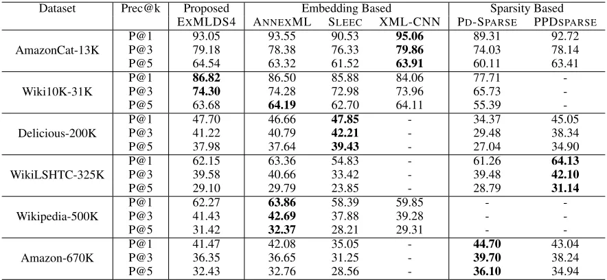
Joint Learning: Our method EXMLDS4 can jointly learn the embedding and regression. To implement joint learning, we modified the existing code of state-of-the-art embedding based extreme classification approach AnnexML (Tagami 2017a)6_{, by replacing theDSSM}7_training

objec-tive by word2vecobjective, while keeping cosine simi-larity, partitioning algorithm, and approximate nearest pre-diction algorithm same. For efficient training of rare label, we keep the coefficient ratio of negative to positive sam-ples as 20:1, while training for all datasets. We used the same hyper-parameters i.e. embedding size as 50, number of learner for each cluster as 15, number of nearest neigh-bor as 10, number of embedding and partitioning iteration both 100, gamma as 1, label normalization as true, num-ber of threads as 32. We obtain state-of-the-art result i.e. similar or better in comparison to DISMEC (Babbar and Sch¨olkopf 2017), PPDSPARSE (Yen et al. 2017) and AN

-NEXML (Tagami 2017b) and SLEEC(Bhatia et al. 2015) on all large datasets, see table 3 for details results. Our training and prediction time for EXMLDS4 was similar to that of ANNEXML.

Analysis and Discussion

Although SLEECperforms slightly better on some datasets, our EXMLDS1 model is much faster than SLEECin training on large datasets as shown in Table 1. The performance of our model EXMLDS3 in Table 4 when a significant fraction of labels missing is considerably better than SLEECand other label embedding based baselines such as LEMLand LEML

-6

Table 2: Comparing prediction performance of different methods(−mean unavailable results). Note that although SLEEC performs slightly better, our model is much faster as shown in the results in Table 1. Also note the performance of our model in Table 4 when a significant fraction of labels are missing is considerably better than SLEEC

Dataset Prec@k Propose Embedding Based Sparsity Tree Based XML Others EXMLDS1 DXML SLEEC LEML PD-SPARSE PFASTRE FAST 1-vs-All DISMEC Bibtex P@1 P@3 P@5 63.38 38.00 27.64 63.69 37.63 27.71 65.29 39.60 28.63 62.54 38.41 28.21 61.29 35.82 25.74 63.46 39.22 29.14 63.42 39.23 28.86 62.62 39.09 28.79 -Delicious P@1 P@3 P@5 67.94 61.35 56.3 67.57 61.15 56.7 68.10 61.78 57.34 65.67 60.55 56.08 51.82 44.18 38.95 67.13 62.33 58.62 69.61 64.12 59.27 65.01 58.88 53.28 -Eurlex P@1 P@3 P@5 77.55 64.18 52.51 77.13 64.21 52.31 79.52 64.27 52.32 63.40 50.35 41.28 76.43 60.37 49.72 75.45 62.70 52.51 71.36 59.90 50.39 79.89 66.01 53.80 82.40 68.50 57.70 Mediamill P@1 P@3 P@5 87.49 72.62 58.46 88.71 71.65 56.81 87.37 72.6 58.39 84.01 67.20 52.80 81.86 62.52 45.11 83.98 67.37 53.02 84.22 67.33 53.04 83.57 65.60 48.57 -Delicious-200K P@1 P@3 P@5 46.07 41.15 38.57 44.13 39.88 37.20 47.50 42.00 39.20 40.73 37.71 35.84 34.37 29.48 27.04 41.72 37.83 35.58 43.07 38.66 36.19 -45.50 38.70 35.50

Table 3: Comparing prediction performance of state-of-the-art embedding based methods (−mean unavailable results) on large dataset with joint learning

Dataset Prec@k Proposed Embedding Based Sparsity Based EXMLDS4 ANNEXML SLEEC XML-CNN PD-SPARSE PPDSPARSE

AmazonCat-13K P@1 P@3 P@5 93.05 79.18 64.54 93.55 78.38 63.32 90.53 76.33 61.52 95.06 79.86 63.91 89.31 74.03 60.11 92.72 78.14 63.41 Wiki10K-31K P@1 P@3 P@5 86.82 74.30 63.68 86.50 74.28 64.19 85.88 72.98 62.70 84.06 73.96 64.11 77.71 65.73 55.39 -Delicious-200K P@1 P@3 P@5 47.70 41.22 37.98 46.66 40.79 37.64 47.85 42.21 39.43 -34.37 29.48 27.04 45.05 38.34 34.90 WikiLSHTC-325K P@1 P@3 P@5 62.15 39.58 29.10 63.36 40.66 29.79 54.83 33.42 23.85 -61.26 39.48 28.79 64.13 42.10 31.14 Wikipedia-500K P@1 P@3 P@5 62.27 41.43 31.42 63.86 42.69 32.37 58.39 37.88 28.21 59.85 39.28 29.31 -Amazon-670K P@1 P@3 P@5 41.47 36.35 32.43 42.08 36.65 32.76 35.05 31.25 28.56 -44.70 39.70 36.10 43.04 38.24 34.94

Table 4: Evaluating competitive methods in the setting where 80%of the training labels are hidden

Data P@k Exmlds3 SLEEC LEML LEML-IMC

Bibtex P@1 P@3 P@5 48.51 28.43 20.7 30.5 14.9 9.81 35.98 21.02 15.50 41.23 25.25 18.56 Eurlex P@1 P@3 P@5 60.28 44.87 35.31 51.4 37.64 29.62 26.22 22.94 19.02 39.24 32.66 26.54 rcv1v2 P@1 P@3 P@5 81.67 52.82 37.74 41.8 17.48 10.63 64.83 42.56 31.68 73.68 48.56 34.82

Conclusions and Future Work

The this paper we establish a connection between

word2vecin NLP with multi-label learning in XML. The benefit leap by the connection is efficient and fast training, easy handling of the missing label using external auxiliary label-label correlation information and easily perform joint embedding learning and regression. Our proposed objective can be optimized efficiently by SPPMImatrix factorization and can also incorporates side information, which is effective in handling missing labels. Through comprehensive experi-ments, we showed that the proposed method is competitive compared to state-of-the-art multi-label learning methods in terms of prediction accuracies. Joint training model learning learn the regressionV which has a large number of entriesd ×L, asLis the number of labels (millions). One can use the sparsity inX (we usedV X), to design better training over the joint model.

References

Babbar, R., and Sch¨olkopf, B. 2017. Dismec: distributed sparse machines for extreme multi-label classification. In

Proceedings of the Tenth ACM International Conference on Web Search and Data Mining, 721–729. ACM.

Bhatia, K.; Jain, H.; Kar, P.; Varma, M.; and Jain, P. 2015. Sparse local embeddings for extreme multi-label classifica-tion. InNIPS, 730–738.

Boyd, S.; Parikh, N.; Chu, E.; Peleato, B.; and Eckstein, J. 2011. Distributed optimization and statistical learning via the alternating direction method of multipliers.Foundations and TrendsR in Machine Learning3(1):1–122.

Dai, A. M.; Olah, C.; and Le, Q. V. 2015. Docu-ment embedding with paragraph vectors. arXiv preprint arXiv:1507.07998.

Hochreiter, S., and Schmidhuber, J. 1997. Long short-term memory.Neural Comput.9(8):1735–1780.

Jain, L. C., and Medsker, L. R. 1999. Recurrent Neural Networks: Design and Applications. Boca Raton, FL, USA: CRC Press, Inc., 1st edition.

Jain, H.; Prabhu, Y.; and Varma, M. 2016. Extreme multi-label loss functions for recommendation, tagging, ranking & other missing label applications. In22nd ACM SIGKDD, 935–944. ACM.

Jasinska, K.; Dembczynski, K.; Busa-Fekete, R.; Pfannschmidt, K.; Klerx, T.; and Hullermeier, E. 2016. Extreme f-measure maximization using sparse probability estimates. InICML, 1435–1444.

Kiros, R.; Zhu, Y.; Salakhutdinov, R. R.; Zemel, R.; Urtasun, R.; Torralba, A.; and Fidler, S. 2015. Skip-thought vectors. InNIPS, 3294–3302.

Le, Q. V., and Mikolov, T. 2014. Distributed representations of sentences and documents. InICML, volume 14, 1188– 1196.

Levy, O., and Goldberg, Y. 2014. Neural word embedding as implicit matrix factorization. InNIPS, 2177–2185.

Liu, J.; Chang, W.-C.; Wu, Y.; and Yang, Y. 2017. Deep learning for extreme multi-label text classification. In40th

International ACM SIGIR Conference, SIGIR ’17, 115–124. New York, NY, USA: ACM.

Mikolov, T.; Sutskever, I.; Chen, K.; Corrado, G. S.; and Dean, J. 2013. Distributed representations of words and phrases and their compositionality. InNIPS, 3111–3119. Pennington, J.; Socher, R.; and Manning, C. D. 2014. Glove: Global vectors for word representation. In EMNLP, vol-ume 14, 1532–1543.

Prabhu, Y., and Varma, M. 2014. Fastxml: A fast, accurate and stable tree-classifier for extreme multi-label learning. In

Proceedings of the 20th ACM SIGKDD, 263–272. ACM. Rifkin, R., and Klautau, A. 2004. In defense of one-vs-all classification. Journal of machine learning research

5(Jan):101–141.

Tagami, Y. 2017a. Annexml: Approximate nearest neighbor search for extreme multi-label classification. InProceedings of the 23rd ACM SIGKDD, KDD ’17, 455–464. New York, NY, USA: ACM.

Tagami, Y. 2017b. Learning extreme multi-label tree-classifier via nearest neighbor graph partitioning. In26th International Conference on World Wide Web Companion, WWW ’17 Companion, 845–846.

Weston, J.; Bengio, S.; and Usunier, N. 2010. Large scale image annotation: learning to rank with joint word-image embeddings. Machine learning81(1):21–35.

Yen, I. E.-H.; Huang, X.; Ravikumar, P.; Zhong, K.; and Dhillon, I. 2016. Pd-sparse: A primal and dual sparse ap-proach to extreme multiclass and multilabel classification. In

ICML, 3069–3077.

Yen, I. E.; Huang, X.; Dai, W.; Ravikumar, P.; Dhillon, I.; and Xing, E. 2017. Ppdsparse: A parallel primal-dual sparse method for extreme classification. InProceedings of the 23rd ACM SIGKDD, KDD ’17, 545–553. New York, NY, USA: ACM.

Yih, W.-t.; Toutanova, K.; Platt, J. C.; and Meek, C. 2011. Learning discriminative projections for text similarity mea-sures. InFifteenth Conference on Computational Natural Language Learning, 247–256. Association for Computa-tional Linguistics.