The Thirty-Third AAAI Conference on Artificial Intelligence (AAAI-19)
Submodular Optimization over Streams with Inhomogeneous Decays
Junzhou Zhao,
1Shuo Shang,
2Pinghui Wang,
3John C.S. Lui,
4Xiangliang Zhang
1∗1King Abdullah University of Science and Technology, KSA
2Inception Institute of Artificial Intelligence, UAE 3Xi’an Jiaotong University, China
4The Chinese University of Hong Kong, Hong Kong
{junzhou.zhao, xiangliang.zhang}@kaust.edu.sa, [email protected], [email protected], [email protected]
Abstract
Cardinality constrained submodular function maximization, which aims to select a subset of size at mostk to maxi-mize a monotone submodular utility function, is the key in many data mining and machine learning applications such as data summarization and maximum coverage problems. When data is given as a stream,streaming submodular optimiza-tion (SSO)techniques are desired. Existing SSO techniques can only apply to insertion-only streams where each element has an infinite lifespan, and sliding-window streams where each element has a same lifespan (i.e., window size). How-ever, elements in some data streams may have arbitrary differ-ent lifespans, and this requires addressing SSO over streams withinhomogeneous-decays(SSO-ID). This work formulates the SSO-ID problem and presents three algorithms: BASIC -STREAMINGis a basic streaming algorithm that achieves an
(1/2−)approximation factor; HISTAPPROXimproves the efficiency significantly and achieves an (1/3−) approx-imation factor; HISTSTREAMING is a streaming version of HISTAPPROXand uses heuristics to further improve the effi-ciency. Experiments conducted on real data demonstrate that HISTSTREAMINGcan find high quality solutions and is up to two orders of magnitude faster than the naive GREEDY algo-rithm.
Introduction
Selecting a subset of data to maximize some utility function under a cardinality constraint is a fundamental problem fac-ing many data minfac-ing and machine learnfac-ing applications. In myriad scenarios, ranging from data summarization (Mitro-vic et al. 2018), to search results diversification (Agrawal et al. 2009), to feature selection (Brown et al. 2012), to cover-age maximization (Cormode, Karloff, and Wirth 2010), util-ity functions commonly satisfysubmodularity(Nemhauser, Wolsey, and Fisher 1978), which captures thediminishing returnsproperty. It is therefore not surprising that submod-ular optimization has attracted a lot of interests in recent years (Krause and Golovin 2014).
If data is given in advance, the GREEDYalgorithm can be applied to solve submodular optimization in abatchmode. However, today’s data could be generated continuously with
∗
Shuo Shang and Xiangliang Zhang are the corresponding au-thors.
Copyright c2019, Association for the Advancement of Artificial Intelligence (www.aaai.org). All rights reserved.
∞∞∞∞∞∞∞∞ t
∞∞∞∞∞∞∞∞∞ t+ 1
insertion-only
remaining lifespan
0 0 0 0 1 2 3 4
t
0 0 0 0 0 1 2 3 4
t+ 1
sliding-window (homogeneous decay)
remaining lifespan
0 1 3 2 0 4 1 5 t
0 0 2 1 0 3 0 4 2 t+ 1
0 0 1 0 0 2 0 3 1 3 t+ 2
inhomogeneous decay
remaining lifespan
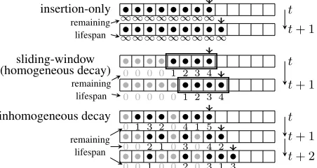
Figure 1:Insertion-only stream: each element has an infi-nite lifespan.Sliding-window stream: each element has a same initial lifespan.Our model: each element can have an arbitrary lifespan.
no ending, and in some cases, data is produced so rapidly that it cannot even be stored in computer main memory, e.g., Twitter generates more than 8,000 tweets every sec-ond (Internet Live Stats 2018). Thus, it is crucial to design
streaming algorithms where at any point of time the algo-rithm has access only to a small fraction of data. To this end,
streaming submodular optimization (SSO)techniques have been developed forinsertion-only streamswhere a subset is selected from all historical data (Badanidiyuru et al. 2014), andsliding-window streamswhere a subset is selected from the most recent data only (Epasto et al. 2017).
data or include many recent but valueless data. Can we de-sign SSO techniques with a better streaming setting?
We observe that both insertion-only stream and sliding-window stream actually can be unified by introducing the concept of datalifespan, which is the amount of time an ele-ment participating in subset selection. As time advances, an element’s remaining lifespan decreases. When an element’s lifespan becomes zero, it is discarded and no longer par-ticipates in subset selection. Specifically, in insertion-only streams, each element has an infinite lifespan and will al-ways participate in subset selection after arrival. While in sliding-window streams, each element has a same initial lifespan (i.e., the window size), and hence participates in subset selection for a same amount of time (see Fig. 1).
We observe that in some real-world scenarios, it may be inappropriate to assume that each element in a data stream has a same lifespan. Let us consider the following scenario.
Motivating Example.Consider a news aggregation website such as Hacker News (Y Combinator 2018) where news sub-mitted by users form a news stream. Interesting news may attract users to keep clicking and commenting and thus sur-vive for a long time; while boring news may only sursur-vive for one or two days (Leskovec, Backstrom, and Kleinberg 2009). In news recommendation tasks, we should select a subset of news fromcurrent alive newsrather than the most recent news.
Therefore, besides timestamp of each data element, lifes-pan of each data element should also be considered in subset selection. Other similar scenarios include hot video selection from YouTube (where each video may have its own lifes-pan), and trending hashtag selection from Twitter (where each hashtag may have a different lifespan).
Overview of Our Approach. We propose to extend the two extreme streaming settings to a more general stream-ing settstream-ing where each element is allowed to have an ar-bitrary initial lifespan and thus each element can partic-ipate in subset selection for an arbitrary amount of time (see Fig. 1). We refer to this more general decaying mech-anism asinhomogeneous decay, in contrast to the homoge-neous decayadopted in sliding-window streams. This work presents three algorithms to address SSO over streams with inhomogeneous decays (SSO-ID). We first present a sim-ple streaming algorithm, i.e., BASICSTREAMING. Then, we present HISTAPPROXto improve the efficiency significantly. Finally, we design a streaming version of HISTAPPROX, i.e., HISTSTREAMING. We theoretically show that our al-gorithms have constant approximation factors.
Our main contributions include:
• We propose a general inhomogeneous-decaying stream-ing model that allows each element to participate in subset selection for an arbitrary amount of time.
• We design three algorithms to address the SSO-ID prob-lem with constant approximation factors.
• We conduct experiments on real data, and the results demonstrate that our method finds high quality solutions and is up to two orders of magnitude faster than GREEDY.
Problem Statement
Data Stream. A data stream comprises an unbounded se-quence of elements arriving in chronological order, denoted by {v1, v2, . . .}. Each element is from set V, called the
ground set, and each elementv has a discrete timestamp tv ∈ N. It is possible that multiple data elements arriving at the same time. In addition, there may be other attributes associated with each element.
Inhomogeneous Decay. We propose an inhomogeneous-decaying data stream(IDS) model to enableinhomogeneous decays. For an elementvarrived at timetv, it is assigned an initiallifespanl(v, tv)∈Nrepresenting the maximum time span that the element will remain active. As time advances to t ≥ tv, the element’sremaining lifespan decreases to l(v, t),l(v, tv)−(t−tv). Ifl(v, t0) = 0at some timet0,vis discarded. We will assumel(v, tv)is given as an input to our algorithm. At any timet, active elements in the stream form a set, denoted bySt,{v:v∈V ∧tv≤t∧l(v, t)>0}.
IDS model is general. Ifl(v, tv) = ∞,∀v, an IDS be-comes an insertion-only stream. Ifl(v, tv) =W,∀v, an IDS becomes a sliding-window stream. Ifl(v, tv)follows a ge-ometric distribution parameterized byp, i.e.,P(l(v, tv) =
l) = (1−p)l−1p, it is equivalent of saying that an active
element is discarded with probabilitypat each time step. To simplify notations, if timetis clear from context, we will uselvto representl(v, t), i.e., the remaining lifespan (or just say “the lifespan”) of elementvat timet.
Monotone Submodular Function (Nemhauser, Wolsey, and Fisher 1978). A set functionf: 2V 7→
R≥0is submod-ular if f(S ∪ {s})−f(S) ≥ f(T ∪ {s})−f(T), for all S ⊆T ⊆V ands∈V\T.fis monotone (non-decreasing) iff(S)≤f(T)for allS ⊆T ⊆V. Without loss of gener-ality, we assumef is normalized, i.e.,f(∅) = 0.
Letδ(s|S),f(S∪{s})−f(S)denote themarginal gain
of adding elementstoS. Then monotonicity is equivalent of saying that the marginal gain of every element is always non-negative, and submodularity is equivalent of saying that marginal gainδ(s|S)of elementsnever increases as setS grows bigger, aka the diminishing returns property.
Streaming Submodular Optimization with Inhomoge-neous Decays (SSO-ID). Equipped with the above no-tations, we formulate the cardinality constrained SSO-ID problem as follows:
OPTt,max
S f(S), s.t. S⊆ St∧ |S| ≤k,
wherekis a given budget.
Algorithms
This section presents three algorithms to address the SSO-ID problem. Due to space limitation, the proofs of all theorems are included in the extended version of this paper.
Warm-up: The B
ASICS
TREAMINGAlgorithm
In the literature, SIEVESTREAMING (Badanidiyuru et al. 2014) is designed to address SSO over insertion-only streams. We leverage SIEVESTREAMING as a basic build-ing block to design a BASICSTREAMING algorithm. BA
-SICSTREAMINGis simple per se and may be inefficient, but offers opportunities for further improvement. This section assumes lifespan is upper bounded byL, i.e.,lv ≤ L,∀v. We later remove this assumption in the following sections.
SIEVESTREAMING(Badanidiyuru et al. 2014) is a thresh-old based streaming algorithm for solving cardinality con-strained SSO over insertion-only streams. The high level idea is that, for each coming element, it is selected only if its gain w.r.t. a set is no less than a threshold. In its im-plementation, SIEVESTREAMING lazily maintains a set of
log1+2k=O(−1logk)thresholds and each is associated with a candidate set initialized empty. For each coming ele-ment, its marginal gain w.r.t. each candidate set is computed; if the gain is no less than the corresponding threshold and the candidate set is not full, the element is added in the candi-date set. At any time, a candicandi-date set having the maximum utility is the current solution. SIEVESTREAMING achieves an(1/2−)approximation guarantee.
Algorithm Description.We show how SIEVESTREAMING
can be used to design a BASICSTREAMING algorithm to solve the SSO-ID problem. LetVtdenote a set of elements arrived at time t. We partition Vt into (at most) L non-overlapping subsets, i.e.,Vt =∪Ll=1V
(t)
l whereV (t) l is the subset of elements with lifespanlat timet. BASICSTREAM
-INGmaintainsLSIEVESTREAMING instances, denoted by {A(t)l }L
l=1, and alternates adata updatestep and atime
up-datestep to process the arriving elementsVt.
•Data Update.This step processes arriving dataVt. Let in-stanceA(t)l only process elements with lifespan no less than
l. In other words, elements in∪i≥lV
(t)
i are fed toA (t) l . After processingVt,A
(t)
1 outputs the current solution.
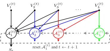
•Time Update.This step prepares for processing the up-coming data in the next time step. We reset instanceA(t)1 , i.e., empty its threshold set and each candidate set. Then we conduct acircular shiftoperation:A(t+1)1 ← A(t)2 ,A(t+1)2 ← A(t)3 , . . . ,A(t+1)L ← A(t)1 .
BASICSTREAMINGalternates the two steps and continu-ously processes data at each time step. We illustrate BASIC -STREAMINGin Fig. 2, with pseudo-code given in Alg. 1.
Analysis.BASICSTREAMING exhibits a feature that an in-stance gradually expires (and is reset) as data processed in it expires. Such a feature ensures that, at any time t, A(t)1 always processed all the data inSt. BecauseA
(t) 1 is a SIEVESTREAMINGinstance, we immediately have the fol-lowing conclusions.
A(1t) A(2t) A(3t) · · · A(Lt)
St
V1(t) V2(t) V3(t) VL(t)
· · ·
resetA(1t)andt←t+ 1
Figure 2: BASICSTREAMING. Solid lines denote data up-date, and dashed lines denote time update.
Algorithm 1:BASICSTREAMING
Input:An IDS of data elements arriving over time
Output:A subsetStat any timet
1 InitializeLSIEVESTREAMINGinstances{A(1)l }L l=1;
2 fort= 1,2, . . .do
3 forl= 1, . . . , LdoFeedA(t)l with data∪i≥lV (t) i ;
4 St←output ofA(t)1 ;
5 forl= 2, . . . , LdoA(t+1)l−1 ← A(t)l ; 6 ResetA(t)1 andA(t+1)L ← A(t)1 ;
Theorem 1. BASICSTREAMINGachieves an(1/2−) ap-proximation guarantee.
Theorem 2. BASICSTREAMING uses O(L−1logk)time to process each element, and O(Lk−1logk) memory to
store intermediate results (i.e., candidate sets).
Remark. As illustrated in Fig. 2, data with lifespanlwill be fed to{A(t)i }i≤l. Hence, elements with large lifespans will fan out to a large fraction of SIEVESTREAMINGinstances, and incur high CPU and memory usage, especially whenL is large. This is the mainbottleneckof BASICSTREAMING. On the other hand, elements with small lifespans only need to be fed to a few instances. Therefore, if data lifespans are mainly distributed over small values, e.g., power-law dis-tributed, then BASICSTREAMINGis still efficient.
H
ISTA
PPROX: Improving Efficiency
To address the bottleneck of BASICSTREAMINGwhen pro-cessing data with a large lifespan, we design HISTAPPROX
in this section. HISTAPPROXcan significantly improve the efficiency of BASICSTREAMINGbut requires active dataSt to be stored in RAM1. Strictly speaking, HISTAPPROX is not a streaming algorithm. We later remove the assumption of storingStin RAM in the next section.
Basic Idea.If at any time, only a few instances are main-tained and running in BASICSTREAMING, then both CPU time and memory usage will decrease. Our idea is hence to selectively maintain a subset of SIEVESTREAMING in-stances that can approximate the rest. Roughly speaking, this
1For example, if lifespan follows a geometric distribution, i.e.,
P(lv =l) = (1−p)pl−1, l= 1,2, . . ., and at mostMelements arrive at a time, then|St| ≤Pt
−1 a=0M p
a≤ M
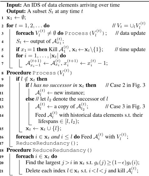
idea can be thought of as using a histogram to approximate a curve. Specifically, letgt(l)denote the value of output of A(t)l at timet. For very largeL, we can think of{gt(l)}l≥1 as a “curve” (e.g., the dashed curve in Fig. 3). Our idea is to pick a few instances asactive instances and construct a histogram to approximate this curve, as illustrated in Fig. 3.
x1 x2 x3 x4 x5
1
Case 1
Case 2 Case 3
{gt(l)}l≥1 {g
t(l)}l∈xt
Figure 3: Approximate{gt(l)}l≥1by{gt(l)}l∈xt.
The challenge is that, as new data keeps arriving, the curve is changing; hence, we need to update the histogram accord-ingly to make sure that the histogram always well approx-imates the curve. Letxt , {x(t)1 , x(t)2 , . . .} index a set of active instances at timet, where each indexx(t)i ≥1.2In the follows, we describe thextupdating method, i.e., HISTAP -PROX, and the method guarantees that the maintained his-togram satisfies our requirement.
Algorithm Description. HISTAPPROX consists of two steps: (1) updating indices; (2) removing redundant indices. •Updating Indices.The algorithm starts with an empty in-dex set, i.e., x1 = ∅. At time t, consider a set of newly arrived elementsVl(t)with lifespan l. These elements will
increase the curve beforel(because dataVl(t)will be fed to {A(t)i }i≤l, see Fig. 2). There are three cases based on the position ofl, as illustrated in Fig. 3.
Case 1. Ifl∈xt, we simply feedVl(t)to{Ai(t)}i∈xt∧i≤l.
Case 2. Ifl /∈xtandlhas no successor inxt, we create a new instanceA(t)l and feedVl(t)to{Ai(t)}i∈xt∧i≤l.
Case 3. Ifl /∈xtandlhas a successorl2∈xt. LetA (t) l be a copy ofA(t)l
2 , then we feedV (t) l to{A
(t)
i }i∈xt∧i≤l. Note
thatA(t)l needs to process all data with lifespan≥lat time
t. BecauseA(t)l
2 has processed all data with lifespan≥l2, we still need to feedA(t)l with historical data s.t. their lifespan ∈[l, l2). That is the reason we needStto be stored in RAM. Above scheme guarantees that each A(t)l , l ∈ xt pro-cessed all the data with lifespan≥lat timet. The detailed pseudo-code is given in procedureProcessof Alg. 2. •Removing Redundant Indices.Intuitively, if the outputs of two instances are close to each other, it is not necessary to keep both of them. We need the following definition to quantify redundancy.
Definition 1 (-redundancy). At time t, consider two in-stancesA(t)i andA(t)l withi < l. We sayA(t)l is-redundant if their existsj > lsuch thatgt(j)≥(1−)gt(i).
The above definition simply states that, since A(t)i and A(t)j are already close with each other, then instances
be-2
Superscripttwill be omitted if timetis clear from context.
Algorithm 2:HISTAPPROX
Input:An IDS of data elements arriving over time
Output:A subsetStat any timet
1 x1← ∅;
2 fort= 1,2, . . .do //Vt=∪lVl(t)
3 foreachVl(t)6=∅doProcess(Vl(t)); // data update
4 St←output ofA(t)x1; 5 ifx1= 1thenKillA (t)
1 ,xt←xt\{1}; // time update
6 fori= 1, . . . ,|xt|do
7 A(t+1)x
i−1 ← A (t) xi,x
(t+1)
i ←x
(t) i −1;
8 ProcedureProcess(Vl(t))
9 ifl /∈xtthen
10 iflhas no successor inxtthen // Case 2 in Fig. 3
11 A(t)l ←new instance;
12 else// letl2denote the successor ofl
13 A(t)l ←a copy ofA(t)l
2; // Case 3 in Fig. 3 14 FeedA(t)l with historical data elements s.t. their
lifespans∈[l, l2);
15 xt←xt∪ {l};
16 foreachi∈xtandi≤ldoFeedA(t)i withVl(t);
17 ReduceRedundancy();
18 ProcedureReduceRedundancy()
19 foreachi∈xtdo
20 Find the largestj > iinxts.t.gt(j)≥(1−)gt(i);
21 Delete each indexl∈xts.t.i < l < jand killA(t)l ;
tween them are redundant. In HISTAPPROX, we regularly check the output of each instance and terminate those redun-dant ones, as described inReduceRedundancyof Alg. 2.
Analysis. Notice that indicesx ∈ xt andx+ 1 ∈ xt−1 are actually the same index (if they both exist) but appear at different time. In general, we sayx0 ∈x
t0 is anancestorof
x∈xtift0 ≤tandx0 =x+t−t0. In the follows, letx0 denotex’s ancestor at timet0. First, HISTAPPROXmaintains a histogram satisfying the following property.
Lemma 1. For two consecutive indicesxi, xi+1∈xtat any timet, one of the following two cases holds:
C1 Stcontains no data with lifespan∈(xi, xi+1).
C2 gt0(x0i+1)≥(1−)gt0(x0i)at some timet0≤t, and from timet0tot, there is no data with lifespan between the two indices arrived (exclusive).
Histogram with property C2 is known as a smooth his-togram (Braverman and Ostrovsky 2007). Smooth his-togram together with the submodularity offare sufficient to ensure a constant factor approximation guarantee ofgt(x1).
Theorem 3. HISTAPPROXis(1/3−)-approximate, i.e., at any timet,gt(x1)≥(1/3−)OPTt.
Theorem 4. HISTAPPROXusesO(−2log2k)
time to pro-cess each coming element and O(k−2log2k) memory to store intermediate results and|St|memory to storeSt.
HISTAPPROXfinds solutions with quality very close to BA
-SICSTREAMINGand is much faster. The main drawback of HISTAPPROX is that active data St needs to be stored in RAM to ensure eachA(t)l ’s output is accurate. IfStis larger than RAM capacity, then HISTAPPROXis inapplicable. We address this limitation in the following section.
H
ISTS
TREAMING: A Heuristic Streaming
Algorithm
Based on HISTAPPROX, this section presents a streaming al-gorithm HISTSTREAMING, which uses heuristics to further improve the efficiency of HISTAPPROX. HISTSTREAMING
no longer requires storing active dataStin memory.
Basic Idea.If we do not need to process the historical data in HISTAPPROX(Line 14), then there is no need to store St. What ifA
(t)
l does not process historical data? Because A(t)l does not process all the data with lifespan≥ l inSt, there will be a bias between its actual outputˆgt(l)and ex-pected outputgt(l). We only need to worry about the case
ˆ
gt(l) < gt(l), as the other casegtˆ(l) ≥ gt(l) means that without processing historical data,A(t)l finds even better so-lutions (which may rarely happen in practice but indeed pos-sible). In the follows, we apply two useful heuristics to de-sign HISTSTREAMING, and show that historical data can be
ignored due to its insignificance and submodularity of ob-jective function.
Effects of historical data.Intuitively, if historical data is in-significant, then a SIEVESTREAMINGinstance may not need to process it at all, and can still output quality guaranteed solutions. We notice that, in HISTAPPROX, a newly created instanceA(t)l essentially needs to process three substreams: (1) elements arrived beforetwith lifespan≤l2(Line 13)3; (2) unprocessed historical elements with lifespan ∈ [l, l2) (Line 14); (3) newly arrived elementsVl(Line 16). Denote these three substreams byS1, S2 andS3, respectively. We state a useful lemma below.
Lemma 2. LetS1kS2kS3denote the concatenation of three
substreamsS1, S2, S3. LetA(S)denote the output value of applying SIEVESTREAMING algorithmA on streamS. If
A(S1) ≥ αA(S1kS2)for 0 < α < 1, then A(S1kS3) ≥
(1/4−)αOPTwhereOPTis the value of an optimal so-lution in streamS1kS2kS3.
Lemma 2 states that, if historical dataS2is insignificant, i.e., A(S1) ≥ αA(S1kS2) for 0 < α < 1 (the closer α is to1, the less significantS2is), then an instance does not need to processS2and still finds quality guaranteed solu-tions. This will further ensure that HISTAPPROXfinds qual-ity guaranteed solutions (more explanation on this point can be found in the extended version of this paper). Although it is intractable to theoretically show that historical dataS2 is indeed insignificant, intuitively, as unprocessed histori-cal dataS2is caused by the deletion of redundant instances (consider the example given in Fig. 4). These instances are
3This substream is actually processed byA(t)
l ’s successorA (t) l2,
and note thatA(t)l is copied fromA(t)l2.
redundant becauseA(S1||S2)does not increase much upon A(S1). Hence, it makes sense to assume that historical data S2is insignificant, and by Lemma 2,S2can be ignored.
l01 l 0
0 l02 l1 l l0 l2
t0 t
Figure 4: At timet0, data with lifespanl0
0arrives and forms a redundant instance, which is removed. At time t > t0, data with lifespanl arrives and A(t)l is created. Data atl0 becomes the unprocessed historical data. We thus say that unprocessed historical data is caused by the deletion of re-dundant instance at previous time.
Protecting non-redundant instances.To further ensure the solution quality of HISTSTREAMING, we introduce another heuristic to protect non-redundant instances.
Because gt(l)is unknown, to avoid removing instances that are actually not redundant, we give each instanceA(t)l an amount of value, denoted by δl, as compensation for not processing historical data, i.e.,gt(l)may be as large as
ˆ
gt(l) +δl. This allows us to representgt(l)by an interval
[gt(l), gt(l)]wheregt(l) , ˆgt(l)andgt(l) , gtˆ(l) +δl. As g
t(j) ≥ (1 −)gt(i) implies gt(j) ≥ (1−)gt(i), the condition in Line 20 of HISTAPPROX is replaced by gt(j)≥(1−)gt(i).
We wantδlto be related to the amount of historical data thatA(t)l does not process. Recall the example in Fig. 4. Un-processed historical data is always fed tol’s predecessor stance whenever redundant instances are removed in the in-tervallbelonging to. Also notice thatgt0(l02)≥(1−)gt0(l10)
holds after the removal of redundant instances. Hence, the contribution of unprocessed historical data can be estimated to be at mostgt0(l01). In general, if some redundant indices
are removed in interval(i, j)at timet, we setδl = gt(i) for indexlthat is later created in the interval(i, j).
Algorithm Description. We only need to slightly modify ProcessandReduceRedundancy(see Alg. 3).
Remark. HISTSTREAMING uses heuristics to further im-prove the efficiency of HISTAPPROX, and no longer needs to storeStin memory. In experiments, we observe that HIST -STREAMINGcan find high quality solutions.
Experiments
In this section, we construct several maximum coverage problems to evaluate the performance of our methods. We use real world and public available datasets. Note that the optimization problems defined on these datasets may seem to be simplistic, as our main purpose is to validate the perfor-mance of proposed algorithms, and hence we want to keep the problem settings as simple and clear as possible.
Datasets
Algorithm 3:HISTSTREAMING
1 ProcedureProcess(Vl(t))
2 ifl /∈xtthen
3 δl←0;
4 · · ·
// Iflhas a successorl2
5 A(t)l ←a copy ofA(t)l 2;
6 Findi, j∈xts.t.l∈(i, j)andδijis recorded, then letδl←δij;
7 · · ·
8 ProcedureReduceRedundancy() 9 foreachi∈xtdo
10 Find the largestj > iinxts.t.g
t(j)≥(1−)gt(i);
11 Delete each indexl∈xts.t.i < l < jand killA(t)l ; // Record the amount of unprocessed data in(i, j) 12 δij←gt(i);
meta information of about3 million papers, including 1.8
million authors and5,079conferences from 1936 to 2018. We say that an author represents a conference if the author published papers in the conference. Our goal is to maintain a small set ofkauthors that jointly represent the maximum number of distinct conferences at any time. We filter out au-thors that published less than10papers and sort the remain-ing188,383 authors by their first publication date to form an author stream. On this dataset, an author’s lifespan could be defined as the time period between its first and last publi-cation dates.
StackExchange. We construct a hot question selection
problem on the math.stackexchange.com website (Stack Exchange 2018). The dataset records about 1.3 million questions with152 thousand commenters from 7/2010to
6/2018. We say a question is hot if it attracts many com-menters to comment. Our goal is select a small set of k questions that jointly attract the maximum number of dis-tinct commenters at any time. The questions are ordered by the post date, and the lifespan of a question can be defined as the time interval length between its post time and last com-ment time.
Settings
Benchmarks. We consider the following two methods as benchmarks.
• GREEDY. We re-run GREEDY on the active data St at each time t, and apply the lazy evaluation trick (Mi-noux 1978) to further improve its efficiency. GREEDYwill serve as an upper bound.
• RANDOM. We randomly pickkelements from active data Stat each timet. RANDOMwill serve as a lower bound.
Efficiency Measure.When evaluating algorithm efficiency, we follow the previous work (Badanidiyuru et al. 2014) and record the number of utility function evaluations, i.e., the number oforacle calls. The advantage of this measure is that it is independent of the concrete algorithm implementation and platform.
Lifespan Generating.In order to test the algorithm perfor-mance under different lifespan distributions, we also con-sider generating data lifespans by sampling from a geomet-ric distribution, i.e.,P(le =l) = (1−p)l−1p, l= 1,2, . . .. Here0< p <1controls the skewness of geometric distribu-tion, i.e., largerpimplies that a data element is more likely to have a small lifespan.
Results
Analyzing BASICSTREAMING.Before comparing the per-formance of our algorithms with benchmarks, let us first study the properties of BASICSTREAMING, as it is the ba-sis of HISTAPPROXand HISTSTREAMING. We mainly
an-alyze how lifespan distribution affects the performance of BASICSTREAMING. To this end, we generate lifespans from
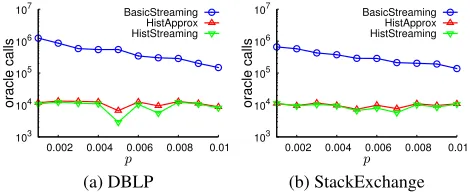
Geo(p) with varyingp, and truncate the lifespan at L = 1,000. We run the three proposed algorithms for100time steps and maintain a set with cardinality k = 10at every time step. We set= 0.1. The solution value and number of oracle calls (at timet = 100) are depicted in Figs. 5 and 6, respectively.
100 200 300 400 500 600
0.002 0.004 0.006 0.008 0.01
value
p BasicStreaming
HistApprox HistStreaming
(a) DBLP
50 60 70 80 90 100 110 120 130
0.002 0.004 0.006 0.008 0.01
value
p BasicStreaming
HistApprox HistStreaming
(b) StackExchange
Figure 5: Solution value comparison (higher is better)
103
104
105
106
107
0.002 0.004 0.006 0.008 0.01
oracle calls
p BasicStreaming
HistApprox HistStreaming
(a) DBLP
103
104
105
106
107
0.002 0.004 0.006 0.008 0.01
oracle calls
p
BasicStreaming HistApprox HistStreaming
(b) StackExchange
Figure 6: Oracle calls comparison (lower is better)
Figure 5 states that the outputs of the three methods are always close with each other under different lifespan dis-tributions, i.e., they always output similar quality solutions. Fig. 6 states that BASICSTREAMING requires much more oracle calls than the other two methods, indicating that BA
most data elements have small lifespans. We also observe that HISTAPPROXand HISTSTREAMINGare not quite sen-sitive to lifetime distribution, and they are much more effi-cient than BASICSTREAMING. In addition, we observe that HISTSTREAMINGis slightly faster than HISTAPPROXeven though HISTSTREAMINGuses smaller RAM.
This experiment demonstrates that BASICSTREAMING, HISTAPPROX, and HISTSTREAMING find solutions with similar quality, but HISTAPPROXand HISTSTREAMINGare much more efficient than BASICSTREAMING.
Performance Over Time. In the next experiment, we fo-cus on analyzing the performance of HISTSTREAMING. We fix the lifespan distribution to be Geo(0.001) with L = 10,000, and run each method for5,000time steps to main-tain a set with cardinality k = 10. Figs. 7 and 8 depict the solution value and ratio of the number of oracle calls (w.r.t. GREEDY), respectively.
0 200 400 600 800 1000 1200
0 1000 2000 3000 4000 5000
value
time Greedy
HistStreaming (ε=0.1) HistStreaming (ε=0.2) Random
(a) DBLP
0 50 100 150 200
0 1000 2000 3000 4000 5000
value
time Greedy
HistStreaming (ε=0.1) HistStreaming (ε=0.2) Random
(b) StackExchange
Figure 7: Solution value over time (higher is better)
0 0.2 0.4 0.6 0.8 1
0 1000 2000 3000 4000 5000
oracle calls ratio
time HistStreaming (ε=0.1) HistStreaming (ε=0.2)
(a) DBLP
0 0.2 0.4 0.6 0.8 1
0 1000 2000 3000 4000 5000
oracle calls ratio
time HistStreaming (ε=0.1) HistStreaming (ε=0.2)
(b) StackExchange
Figure 8: Oracle calls ratio over time (lower is better)
Figure 7 shows that GREEDYand RANDOMalways find the best and worst solutions, respectively, which is expected. HISTSTREAMINGfinds solutions that are close to GREEDY. Smallcan further improve the solution quality. In Fig. 8, we show the ratio of cumulative number of oracle calls be-tween HISTSTREAMINGand GREEDY. It is clear to see that HISTSTREAMINGuses quite a small number of oracle calls comparing with GREEDY. Larger further improves effi-ciency, and for = 0.2the speedup of HISTSTREAMING
could be up to two orders of magnitude faster than GREEDY. This experiment demonstrates that HISTSTREAMING
finds solutions with quality close to GREEDY and is much more efficient than GREEDY.can trade off between solu-tion quality and computasolu-tional efficiency.
Performance under Different Budget k. Finally, we conduct experiments to study the performance of HIST -STREAMINGunder different budgetk. Here, we choose the lifespan distribution as the same as the previous experiment, and set = 0.2. We run HISTSTREAMING and GREEDY
for1000time steps and compute the ratios of solution value and number of oracle calls between HISTSTREAMINGand GREEDY. The results are depicted in Fig. 9.
0 0.2 0.4 0.6 0.8 1
20 40 60 80 100
ratio
k value oracle calls
(a) DBLP
0 0.2 0.4 0.6 0.8 1
20 40 60 80 100
ratio
k value oracle calls
(b) StackExchange
Figure 9: Ratios under different budgetk
In general, using different budgets, HISTSTREAMING al-ways finds solutions that are close to GREEDY, i.e., larger than80%; but uses very few oracle calls, i.e., less than10%. Hence, we conclude that HISTSTREAMINGfinds solutions with similar quality to GREEDY, but is much efficient than GREEDY, under different budgets.
Related Work
Cardinality Constrained Submodular Function Maxi-mization.Submodular optimization lies at the core of many data mining and machine learning applications. Because the objectives in many optimization problems have a di-minishing returns property, which can be captured by sub-modularity. In the past few years, submodular optimization has been applied to a wide variety of scenarios, including sensor placement (Krause, Singh, and Guestrin 2008), out-break detection (Leskovec et al. 2007), search result diver-sification (Agrawal et al. 2009), feature selection (Brown et al. 2012), data summarization (Mirzasoleiman et al. 2015; Mitrovic et al. 2018), influence maximization (Kempe, Kleinberg, and Tardos 2003), just name a few. The GREEDY
algorithm (Nemhauser, Wolsey, and Fisher 1978) plays as a silver bullet in solving the cardinality constrained sub-modular maximization problem. Improving the efficiency of GREEDY algorithm has also gained a lot of interests, such as lazy evaluation (Minoux 1978), disk-based opti-mization (Cormode, Karloff, and Wirth 2010), distributed computation (Epasto, Mirrokni, and Zadimoghaddam 2017; Kumar et al. 2013), sampling (Mirzasoleiman et al. 2015), etc.
few rounds which is suitable for the MapReduce framework. Badanidiyuru et al. (2014) then design the SIEVESTREAM
-ING algorithm which is the first one round streaming al-gorithm for insertion-only streams. SIEVESTREAMING is adopted as the basic building block in our algorithms. SSO over sliding-window streams has recently been studied by Chen et al. (2016) and Epasto et al. (2017) respectively, that both leverage smooth histograms (Braverman and Ostrovsky 2007). Our algorithms actually can be viewed as a general-ization of these existing methods, and our SSO techniques apply for streams with inhomogeneous decays.
Streaming Models. The sliding-window streaming model is proposed by Datar et al. (2002). Cohen et al. (2006) later extend the sliding-window model to general time-decaying model for the purpose of approximating summation aggre-gates in data streams (e.g., count the number of1’s in a01
stream). Cormode et al. (2009) consider the similar estima-tion problem by designing time-decaying sketches. These studies have inspired us to propose the IDS model.
Conclusion
When a data stream consists of elements with different lifespans, existing SSO techniques become inapplicable. This work formulates the SSO-ID problem, and presents three new SSO techniques to address the SSO-ID problem. BASICSTREAMING is simple and achieves an (1/2 −)
approximation factor, but it may be inefficient. HISTAP
-PROX improves the efficiency of BASICSTREAMING sig-nificantly and achieves an (1/3 −) approximation fac-tor, but it requires additional memory to store active data. HISTSTREAMINGuses heuristics to further improve the ef-ficiency of HISTAPPROX, and no longer requires storing ac-tive data in memory. In practice, if memory is not a prob-lem, we suggest using HISTAPPROXas it has a provable ap-proximation guarantee; otherwise, HISTSTREAMINGis also a good choice.
Acknowledgment
We would like to thank the anonymous reviewers for their valuable comments and suggestions to help us improve this paper. This work is financially supported by the King Abdul-lah University of Science and Technology (KAUST) Sensor Initiative, Saudi Arabia. The work of John C.S. Lui was sup-ported in part by the GRF Funding 14208816.
References
Agrawal, R.; Gollapudi, S.; Halverson, A.; and Ieong, S. 2009. Diversifying search results. InWSDM, WSDM. Badanidiyuru, A.; Mirzasoleiman, B.; Karbasi, A.; and Krause, A. 2014. Streaming submodular maximization: Massive data summarization on the fly. InKDD.
Braverman, V., and Ostrovsky, R. 2007. Smooth histograms for sliding windows. InFOCS.
Brown, G.; Pocock, A.; Zhao, M.-J.; and Luj´an, M. 2012. Conditional likelihood maximisation: A unifying framework for information theoretic feature selection.JMLR13:27–66.
Chen, J.; Nguyen, H. L.; and Zhang, Q. 2016. Submodular maximization over sliding windows. InarXiv:1611.00129. Cohen, E., and Strauss, M. J. 2006. Maintaining time-decaying stream aggregates. Journal of Algorithms59:19– 36.
Cormode, G.; Karloff, H.; and Wirth, A. 2010. Set cover algorithms for very large datasets. InCIKM.
Cormode, G.; Tirthapura, S.; and Xu, B. 2009. Time-decaying sketches for robust aggregation of sensor data.
SIAM Journal on Computing39(4):1309–1339.
Datar, M.; Gionis, A.; Indyk, P.; and Motwani, R. 2002. Maintaining stream statistics over sliding windows. SIAM Journal on Computing31(6):1794–1813.
DBLP. 2018. Computer science bibliography. http://dblp. dagstuhl.de/.
Epasto, A.; Lattanzi, S.; Vassilvitskii, S.; and Zadimoghad-dam, M. 2017. Submodular optimization over sliding win-dows. InWWW.
Epasto, A.; Mirrokni, V.; and Zadimoghaddam, M. 2017. Bicriteria distributed submodular maximization in a few rounds. InSPAA.
Internet Live Stats. 2018. Tweets per second. http://www. internetlivestats.com/one-second.
Kempe, D.; Kleinberg, J.; and Tardos, E. 2003. Maximizing the spread of influence through a social network. InKDD. Krause, A., and Golovin, D. 2014. Submodular func-tion maximizafunc-tion. In Tractability: Practical Approaches to Hard Problems. Cambridge University Press.
Krause, A.; Singh, A.; and Guestrin, C. 2008. Near-optimal sensor placements in Gaussian processes: Theory, efficient algorithms and empirical studies. JMLR9:235–284. Kumar, R.; Moseley, B.; Vassilvitskii, S.; and Vattani, A. 2013. Fast greedy algorithms in MapReduce and streaming. InSPAA.
Leskovec, J.; Backstrom, L.; and Kleinberg, J. 2009. Meme-tracking and the dynamics of the news cycle. InKDD. Leskovec, J.; Krause, A.; Guestrin, C.; Faloutsos, C.; Van-Briesen, J.; and Glance, N. 2007. Cost-effective outbreak detection in networks. InKDD.
Minoux, M. 1978. Accelerated greedy algorithms for max-imizing submodular set functions. Optimization Techniques
7:234–243.
Mirzasoleiman, B.; Badanidiyuru, A.; Karbasi, A.; Vondrak, J.; and Krause, A. 2015. Lazier than lazy greedy. InAAAI. Mitrovic, M.; Kazemi, E.; Zadimoghaddam, M.; and Kar-basi, A. 2018. Data summarization at scale: A two-stage submodular approach. InICML.
Nemhauser, G.; Wolsey, L.; and Fisher, M. 1978. An analy-sis of approximations for maximizing submodular set func-tions - I. Mathematical Programming14:265–294.
Stack Exchange. 2018. Stack Exchange data dump. https: //archive.org/details/stackexchange.