Study the Dynamics and Variability of River Indus Flow





This article is published under the terms of the Creative Commons Attribution License 4.0 Author(s) retain the copyright of this article. Publication rights with Alkhaer Publications. Published at: http://www.ijsciences.com/pub/issue/2019-05/

DOI: 10.18483/ijSci.2072; Online ISSN: 2305-3925; Print ISSN: 2410-4477

Study the Dynamics and Variability of River

Indus Flow

Ambreen Javed

, Syed Ahmad Hassan



1

Department of Mathematics Jinnah University for Women, Karachi

2

Department of Mathematics, University of Karachi, Karachi-75270, Pakistan

Abstract: The impact of climate on water, environment and biodiversity is a conventional fact and can be observed throughout the world, especially each south Asian region like Pakistan. The Indus River region of Pakistan is going through phenomenal changes due to climate variations: persistent heat waves, recurring sultry cyclones, frequent floods and prolonged droughts. Floods are one of the important reasons for the life loss, damages of the globe. Pakistan faces large amounts of catastrophic flooding from the past 30 or 35 years, due to the influences of their variability, the dynamics and uncertainty owing to monsoon rainfalls and snow/glacier melts or combination of both. To study the impact of the dynamics and variability a profound mathematical analysis of local temperature and rainfall change projections, in unexpected variations of river flow is essential. This paper provides the realistic approaches by utilizing trend analysis using the techniques of least square estimation and nonparametric Mann-Kendall test and also incorporates multiple linear regression technique (MLR) based on step-wise method. Trend analysis is an important tool used to enumerate and elucidate the dynamics of the hydroclimatic stochastic system. MLR is a mathematical modelling method, used to explain the interrelations of the phenomena and explore their variation relative to the other dependent variable. These methods employed twenty-seven year data of Indus River flows (seven stations), precipitation (four cites) and temperature (three cites). The results show decline of rainfall and rising trend of temperature found in most of the cities, whereas, good explanation of the river flow establishes with MLR in upper stations. The results of this paper may help to understand the space-time dynamics and variability of river flow phenomena. Moreover, It will be useful for agriculture, hydropower generation and water management sectors in planning the future scenarios and forecasting of leading catastrophic occasions.

Keywords: Indus River, Trend, Dynamics, Temperature, Rainfall, MLR

1 Introduction

Withdrawing water from the Himalaya-Karakoram-Hindukush is crucial for hydropower generation agriculture production system, industries and also for domestic use in Pakistan [1]. The impact of climate on water, environment and biodiversity is a conventional fact and can be observed throughout the world. The whole region of the Indus River, Pakistan, is going through phenomenal changes due to climate, which includes persistent heat waves, recurring sultry cyclones, frequent floods and prolonged droughts. Floods are one of the important reasons for the life loss, damages on the globe. This behaviour is similar and is found in nearly each south Asian region [2]. The frequency and magnitude of the catastrophic floods is increased, over the past 30 to 35 years, due to the influences of their variability, the dynamics and uncertainty [3, 4]. Major causes of variability of water circulation in the rivers are the unpredictable climatic behaviour and the natural variability of monsoon rainfall and temperature [2]. Chronological variations and trend evaluation in these river flows in the context of climatic parameters are usually complex. This is because of the nonlinear, cyclical and other temporary instable behaviour and the deficiency and inaccuracy in the river flow data

values. For example, due to the modifications in instruments and observing techniques and most importantly due to the change in location of the meteorological stations and river gauge stations [5]. Therefore, a complete assessment of the significant hydroclimatic variables in the normal state is usually missing [1, 6].

Study the Dynamics and Variability of River Indus Flow

http://www.ijSciences.com

Volume 8 – May 2019 (05)

31

dynamics and variability of Indus River that helped to take possible action to reduce the damages of the flood environmental management, a wide scope covering various interlinked policies. Moreover, it also reviews the role played by different factors in the dynamics and variability of Indus River flow and will contribute in understandings of their future projections. Regression analysis and trend detection of a phenomena based on climate has involved the attention of masses for a long period of time. This paper will discuss in detail the simple methods of trend detection using the techniques of least square estimation and Mann-Kendall test and also incorporates multiple linear regression technique. Trend analysis is an important tool used for determining the behaviour (generally increasing or decreasing) of statistical variations of a random variable. It can be demarcated as the procedure to enumerate and elucidate the changes in any stochastic system for the given epoch of time scale. Regression is a mathematical modelling method, used to explain the interrelations of the phenomena. The two step regression method (step-wise and general regression) have been utilised in this paper. Twenty seven years of mean monthly data of the seven stations of Indus River flow have been used to explore their connection with the, mean monthly temperature of the three cities and the four cities of sum of monthly precipitation. The results of this paper may help to understand the physical phenomena based on the statistical variation with respect to time and space in the river flow. Moreover, It will be useful for agriculture, hydropower generation and water management sectors in planning the future scenarios.

2 Data and Methodology

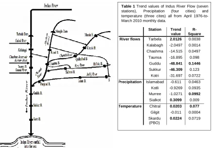
This paper utilizes, the mean monthly river flow data from April 1976 to March 2010 (27 years), for seven different stations, Tarbela, Kalabagh, Chashma, Taunsa, Guddu, Sukkur and Kotri along the Indus River (Fig. 1) are taken from Pakistan Water and Development Authority (WAPDA). The same epoch of local climate (Mean monthly temperature and sum of monthly precipitation) data are being used of three temperature (Chitral, Gilgit & Skardu) and four

precipitation (Islamabad, Kotli, Murree & Sialkot) cities, in the coordination of Pakistan Meteorological Department (PMD). Twenty seven years of mean monthly data of the same seven stations of Indus River flow have been used to explore their connection with the, mean monthly temperature of the three cities and the four cities of sum of monthly precipitation.

A common trend of vulnerability in the context of river flow that can be seen at both the stations (Kalabagh and Guddu) along the Indus River [1]. This is because a western tributary of Kabul River meets Indus before Kalabagh station and the four eastern Rivers (Sutlej, Chenab, Ravi & Jhelum) merges in the Indus at Mithankot (before Guddu). Several studies have been conducted in the past to investigate the trend of mean monthly river flow of the Indus Basin. This study extends to the river flow data of seven stations along the lower Indus Basin for evaluation of trend. The aim is to identify the movements and other seasonal patterns of changes in both timings and magnitude of river flow runoff. Trends in the annual river flow were investigated for stations at Tarbela, Kalabagh, Chashma, Taunsa, Guddu, Sukkur and Kotri of the Indus River. Along this sum of annual precipitation data of Islamabad, Kotli, Murree and Sialkot and mean monthly temperature data of the three cities (Chitral, Gilgit and Skardu) are analysed. The trend analysis has been performed by fitting a least square linear trend line to the annual seasonal pattern assessing the significance of the trend using the R-Squared estimate.

Study the Dynamics and Variability of River Indus Flow

http://www.ijSciences.com

Volume 8 – May 2019 (05)

32

Figure 1 Schematic diagram of different Stations along the Indus River flow and its tributaries

2.1 Parametric Trend analysis

Trend analysis of a river flow in the context of magnitude and timings provides a frame work on trends and variability of climate and glacier outflow [7]. It can be demarcated as the procedure to enumerate and elucidate the changes in any stochastic system for the given epoch of time scale. Trend analysis is an important tool used for determining the behaviour (generally increasing or decreasing) of statistical variations of a random variable. Chronological variations and trend evaluation in the

context of hydro-climatic parameters are usually complex. This is because of the nonlinear, cyclical and other temporary instable behaviour and the deficiency and inaccuracy in the river flow data values. For example due to the modifications in instruments and observation techniques and most importantly because of the change in the location of the meteorological stations and river gauge stations [5]. Therefore, a complete assessment of the significant hydro-climatic variables in the normal state is usually missing [1].

Table 1 Trend values of Indus River Flow (seven stations), Precipitation (four cities) and temperature (three cites) all from April 1976-to-March 2010 monthly data.

Station Trend

value R- Square

River flows Tarbela 2.0126 0.0038

Kalabagh -2.0497 0.0014

Chashma -14.515 0.0497

Taunsa -16.895 0.098

Guddu -48.841 0.1446

Sukkur -46.309 0.123

Kotri -31.697 0.0722

Precipitation Islamabad -0.611 0.0463

Kotli -0.9269 0.0935

Murree -1.0271 0.0992

Sialkot 0.3099 0.009

Temperature Chitral 0.0203 0.077

Gilgit -0.011 0.0004

Skardu (PBO)

Study the Dynamics and Variability of River Indus Flow

http://www.ijSciences.com

Volume 8 – May 2019 (05)

33

Figure 2 Trend analysis of (a) Tarbela (b)Kalabagh (c) Chashma (d) Taunsa (e)Guddu (f) Sukkur (g) Kotri station along the Indus River for 1976-2003.

At least 5C rise in temperature is expected to observe in the temperature of the Indus Channel by the end of the 21st Century (based on observation from last three decades) [8]. Consequently, the water requirements for domestic, and crop production will rise 1.5 times above the present need. Therefore, the consistent decreasing trend (as proceeding downwards stations along the Indus River) in annual flow has been found (Fig.2b – g, Table 1) at all stations except at Tarbela (Fig. 2a, Table 1). The

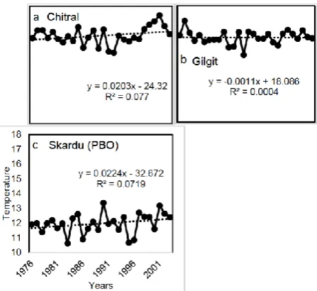
same trend of decreasing behaviour found in three cities of annual rainfall (Fig. 3a-c, Table 1) with the exception of Sialkot (Fig. 3d, Table 1). The Chitral and Skardu has an increasing behaviour with almost same trend values, while the Gilgit city have relatively low value of trend (Fig. 4, Table 1). All these trend behaviours effect directly on the declining behaviour of Indus River flow trend as the increase in temperature may lower down the trend of river flow because of the phenomena of evaporation.

Study the Dynamics and Variability of River Indus Flow

http://www.ijSciences.com

Volume 8 – May 2019 (05)

34

Figure 4 Analysis of trend of Temperature of (a)

Chitral (b) Gilgit (c) Skardu for the years 1976-2003.

2.2 Nonparametric Mann-Kendall test

Trend analysis of hydrological data can be conducted using various methods. They include the techniques of parametric (discussed above) along with non-parametric test (Mann-Kendall). The aim to use the Mann-Kendall test is to statistically investigate the presence of monotonic behaviour of trend on the given data set. If there is an upward trend found, then it implies that the data points are continuously increasing over time and vice versa. The Mann-Kendall test generally notifies the significant variation and their quantification. It has the advantages like no requirement of normally distributed data and no restriction for trend to be linear [9].

The Mann-Kendall test and its magnitude is calculated using the Sen’s approach by utilizes the ‘MAKESENS’ software. The test statistics S used in the Mann-Kendall test is defined as:

S = ∑

∑ ( )

Sign ( ) = {

( )

( )

( )

The statistics S represents the direction of trend. Positive value denotes the increasing trend behaviour of data and vice versa. Mann-Kendall test also states that if the time series has 10 or more data points then the S statistics is approximated by normally distribution with variance defined as:

Var(S) [( ( ) )] ∑ ( )( )

Here m represents the number of classes under consideration and is the size of the ith class. Test statistics Z is calculated as:

Z=

{

_{√ ( )}

√ ( )

In MAKESENS software, the presence of significant trend is computed using the Z statistics. This test value is used to check the null hypothesis (Ho) i.e.; no

trend is present. Positive value of Z indicates the existence of an increasing trend, while the decreasing trend is shown by the negative value of the test statistics Z. The different values at which the significance level has been tested are 0.001, 0.01, 0.05 and 0.1. The slope of the trend Qi recorded using

Mann-Kendall technique is now estimated using the Sen’s slope method as:

Qi =

Here a > b, the long term trends of the seven stations of the Indus River flow (Table 2) reveals that the river flow runoff is in general declining in almost all the stations with a significant decrease in bottom three stations (Kotri, Sukkur and Guddu). But an exceptionally increasing trend observed at Tarbela Station, outflow of the Upper Indus Basin, probably because of the increasing trend in temperature dependent melting of snow glacier of Himalaya-Karakorum-Hindukush Ranges and Monsoon precipitation.

Table 2 Mann-Kendall Trend Statistics of seven stations of Indus River (April 1976-to-March 2010)

Station Test Z

Level of Significance

Q- Slope

B- Intercept

Tarbela 0.18 >0.1 1.622 2302.71

Kalabagh

-0.26 >0.1 -2.545 3200.57

Chashma

-0.53 >0.1 -6.993 3206.98

Taunsa

-1.09 >0.1

-18.412 2974.74

Guddu

-1.84 =0.1

-48.498 3589.77

Sukkur

-1.68 =0.1

-42.989 2431.84

Kotri

-1.53 >0.1

-33.811 1494092

Study the Dynamics and Variability of River Indus Flow

http://www.ijSciences.com

Volume 8 – May 2019 (05)

35

the flood which is a main cause of damage to infrastructure, human being and crops. Therefore, it is required to understand and analyse the river flow runoff system and its relationship with the climatic factors to forecast the future projections of river flow [10]. This paper also investigates the interrelationship of river flow with precipitation and temperature for

different hydrological stations of Indus River as seen from the correlation Table 3 and their seasonal graph Fig. 5. It includes the technique of the general regression method, followed by suggesting the models using step-wise regression analysis. This method may help to identify the possible relationship of climatic parameters and river flow.

Table 3 Correlation of precipitation and temperature cities with seven stations of the Indus River flow (April 1976-to-March 2010).

Stations Rainfall Cities Temperature Cities Islamabad Kotli Murree Sialkot Chitral Gilgit Skardu(PBO)

Tarbela 0.685 0.607 0.558 0.668 0.834 0.807 0.810

Kalabagh 0.689 0.614 0.581 0.675 0.858 0.835 0.836

Chashma 0.700 0.625 0.592 0.686 0.850 0.829 0.830

Taunsa 0.720 0.648 0.608 0.710 0.812 0.7912 0.792

Guddu 0.672 0.628 0.571 0.707 0.652 0.644 0.644

Sukkur 0.644 0.601 0.542 0.689 0.585 0.579 0.579

Kotri 0.571 0.482 0.428 0.593 0.478 0.481 0.480

2.3 Multiple Regression (MLR) Step-wise method

Step-wise regression is an iterative method and an automated tool used in the exploratory stages of building linear regression model from a subset of different independent variables. It helps to identify the useful and optimised subset of predictors. The method works by systematic addition of the most significant variable or removal of the least significant variable during each step. The step-wise regression outputs the most significant models using R-squared (Square of correlation between observed data and model equation) and Adjusted R-squared criterion. Standard step-wise regression both adds and removes predictors as needed for each step. The only requirements of this method are that the data is normally distributed (or rather, that the residuals are), and that there is no correlation between the independent variables (known as collinearity).

Consequently, River flow regression models are produced using step-wise

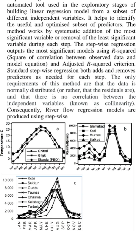
Fig. 5 Seasonal behaviour from Jan 1976-Dec2003. (a) Sum of monthly temperature of three cities and (b) Mean monthly rainfall of four cities (c) Indus River flow seven stations (Tarbela, Kalabagh, Chashma, Taunsa, Guddu, Sukkur, Kotri) in m3/sec..

regression scheme to the monthly river flow data along with the temperature and precipitation components.. This method is used to obtain the optimal regression model for seasonal flow Q in all the seven stations of Indus River.

Q t = Q(ti) +  Ps +  Tr (1)

Here Qt represents the average river flow at each

station, P and S represents the amount of precipitation and temperature accumulated over the given period of time respectively, of the optimal suggested model. The subscripts s and t representing the name of the cities’ precipitation and temperature respectively. If any particular variable has higher p -value (area beyond t-value) , it is eliminated from the model. This p-value of each variable depends on the t-test value which determines whether any variable should be added or eliminated from the suggested model. The resulting optimal estimated regression models are enlisted in Table 4. After the selection of the appropriate model the MLR scheme is applied.

In the MLR method, the case where the dependent variable (River flow) Yn depends upon two or more

independent variables (X1, X2, X3 …etc.) represented

as:

Ŷn =βo + β1 X1 + β2 X2 + β3 X3 +…+ βq Xq (2)

Where β0 is the intercept and β1, β2, β3 are the

Study the Dynamics and Variability of River Indus Flow

http://www.ijSciences.com

Volume 8 – May 2019 (05)

36

equations must be formed with q unknowns.

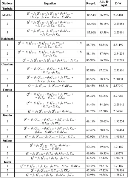
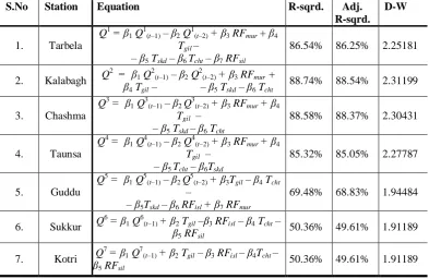
Table 4 Step-wise regression analysis of Indus River flow (April 1976-to-March 2003) based on R -squared, adjusted R-squared and Durban Watson

(DW) criteria. Where RFmur, RFisl , RFsil are the

monthly sum of rainfall at Murree, Islamabad, and Sialkot respectively and Tgil, Tcht and Tskdrepresents

the mean monthly temperature of Gilgit, Chitral and

Skardu respectively

Stations Equation R-sqrd. Adj.

R-sqrd. D-W Tarbela

Model-1 Q

1

= β1 Q1(t–1) – β2 Q1(t–2) + β3 RFmur +

+ β4 Tgil – β5 Tskd – β6Tcht – β7 RFsil

86.54% 86.25% 2.25181

2 Q

1

= β1 Q1(t–1) – β2 Q1(t–2) + β3 RFmur +

+ β4 Tgil – β5 Tskd – β6Tcht

86.40% 86.15% 2.29484

3 Q

1

= β1 Q1(t–1) – β2 Q1(t–2) + β3 RFmur +

+ β4 Tgil – β5 Tskd

85.80% 85.58% 2.23691

Kalabagh

1 Q

2

= β1 Q2(t–1) – β2 Q2(t–2) + β3 RFmur+ + β4

Tgil – β5 Tskd – β6 Tcht

88.74% 88.54% 2.31199

2 Q

2

= β1 Q2(t–1) – β2 Q2(t–2) + β3 RFmur+ + β4

Tgil – β5 Tskd 88.14% 87.96% 2.34234

3 Q2 = β1 Q2(t–1) – β2 Q2(t–2) + β3 RFmur + β4 Tgil 86.92% 86.76% 2.37218

Chashma

1 Q

3

= β1 Q3(t–1) – β2Q3(t–2) + β3 RFmur +

+ β4 Tgil - β5 Tskd 87.81% 87.62% 2.33801

2 Q

3

= β1 Q3(t–1) – β2Q3(t–2) + β3 RFmur +

+ β4 Tgil – β5 Tskd – β6 Tcht 88.58% 88.37% 2.30431

3 Q3 = β1 Q3(t–1) – β2Q3(t–2) + β3 RFmur 86.43% 86.31% 2.37940

Taunsa

1 Q

4

= β1 Q4(t–1) – β2 Q4(t–2) + β3 RFmur +

+ β4 Tgil – β5Tcht – β6Tskd

85.32% 85.05% 2.27787

2

Q4 = β1 Q4(t–1) – β2 Q4(t–2) + β3 RFmur +

+ β4 Tgil – β5Tcht 84.49% 84.26% 2.29142

3 Q4 = β1 Q4(t–1) – β2 Q4(t–2) + β3 RFmur 82.75% 82.60% 2.34368

Guddu

1 Q

5

= β1 Q5(t–1) – β2Q5(t–2) + β3Tgil – β4 Tcht –

– β5Tskd – β6 RFisl

69.19% 68.62% 1.92254

2 Q

5

= β1 Q5(t–1) – β2Q5(t–2) + β3Tgil – β4 Tcht –

– β5Tskd – β6 RFisl + β7 RFmur

69.48% 68.83% 1.94484

3 Q5 = β1 Q5(t–1) – β2Q5(t–2) + β3Tgil – β4 Tcht 67.92% 67.54% 1.95415

Sukkur

1 Q

6

= β1 Q6(t–1) + β2 Tgil –β3 RFisl –

– β4 Tcht – β5 RFsil

50.36% 49.61% 1.91189

2 Q6 = β1 Q6(t–1) + β2 Tgil –β3 RFisl – β4 Tcht 49.95% 49.35% 1.88274

3 Q6 = β1 Q6(t–1) + β2 Tgil –β3 RFisl 47.59% 47.12% 1.88274

Kotri

1 Q7 = β1 Q7(t–1) + β2 Tgil – β3 RFisl – β4Tcht – β5 RFisl 50.36% 49.61% 1.91189

2 Q7 = β1 Q7(t–1) + β2 Tgil – β3 RFisl 47.59% 47.12% 1.78308

Study the Dynamics and Variability of River Indus Flow

http://www.ijSciences.com

Volume 8 – May 2019 (05)

37

climatic parameters and previous river flow runoff Minitab 16 software has been used. The resultant regression models of each stations (Table 5) expresses a very strong impact of the climatic parameters on the Indus River flow. Models of the upstream stations shows strong relation between the variables explaining almost 90% (R-squared and adjusted-R squared values) of the real river flow data. These results show an established relationship between the river flow and climatic parameters and can be used as a tool for estimation of the whole network river flow. These regression models (Table 5), provide suitable information to forecast the future values by considering the climatic factors as independent variables.

However, as move downstream stations along the Indus River, the appropriate regression model

explaining river flow gradually getting weaker, possessing low R-squared values as compared to the upstream stations. This is because of entrance of four eastern Rivers (Jhelum, Chenab, Ravi & Punjand) into the Indus River before Guddu station (Fig. 1). These eastern rivers have seasonal rising time are lagging as compared to the main Indus River, which may weaken the regression relationship of the lower Indus stations.

Table 5 Best selected MLR models of each seven station of Indus River (April 1976-to-March 2003) from Table 4, based on R-squared, adjusted R -squared and Durbin-Watson (D-W) values. Where RFmur, RFisl, RFsil are the monthly sum of rainfall at

Murree, Islamabad, and Sialkot respectively and Tgil,

Tcht and Tskdrepresents the mean monthly temperature

of Gilgit, Chitral and Skardu respectively.

S.No Station Equation R-sqrd. Adj. R-sqrd.

D-W

1. Tarbela

Q1 = β1 Q1(t–1) – β2 Q1(t–2) + β3 RFmur+ β4

Tgil –

– β5 Tskd – β6Tcht – β7 RFsil

86.54% 86.25% 2.25181

2. Kalabagh Q

2

= β1 Q2(t–1) – β2 Q2(t–2) + β3 RFmur +

β4 Tgil – – β5 Tskd – β6 Tcht

88.74% 88.54% 2.31199

3. Chashma

Q3 = β1 Q3(t–1) – β2Q3(t–2) + β3 RFmur + β4

Tgil –

– β5 Tskd – β6 Tcht

88.58% 88.37% 2.30431

4. Taunsa

Q4 = β1 Q4(t–1) – β2 Q4(t–2) + β3 RFmur + β4

Tgil –

– β5Tcht – β6Tskd

85.32% 85.05% 2.27787

5. Guddu

Q5 = β1 Q5(t–1) – β2Q5(t–2) + β3Tgil – β4 Tcht

–

– β5Tskd – β6 RFisl + β7 RFmur

69.48% 68.83% 1.94484

6. Sukkur Q

6

= β1 Q6(t–1) + β2 Tgil –β3 RFisl – β4 Tcht –

β5 RFsil 50.36% 49.61% 1.91189

7. Kotri Q

7

= β1 Q7(t–1) + β2 Tgil – β3 RFisl – β4Tcht –

β5 RFsil 50.36% 49.61% 1.91189

3 Results and Discussion

The trend analysis of hydroclimatic data has been perform by fitting a least square linear trend line to the monthly time series data. The examining graphical behaviour of trend (slope) and R-squared value, as well as it utilizes the non-parametric Mann-Kendall test which investigates the monotonic behaviour of trend for only river flow data. The river flow analysis shows that only Tarbela (2.0126) station shows some increasing trend and all its downstream stations Kalabagh 2.049), Chashma (-14.515), Taunsa (-16.895), Guddu (-48.841), Sukkur (-46.309), Kotri (-31.697) displays consistent growth of decreasing trend (Fig. 2, Table 1). The rising trend of Tarbela may be due to overall increasing trend of temperature (Fig. 4, Table 1) which provide more

Study the Dynamics and Variability of River Indus Flow

http://www.ijSciences.com

Volume 8 – May 2019 (05)

38

consequence of the dependence of climate. The upward three cities (Fig. 3, Table 1) of precipitation, Islamabad (0.611), Kotli (0.926), and Murree (1.027) have considerably negative trend. However, the fourth station Sialkot precipitation has an increasing trend of 0.309. At most of the time, the Sialkot and its neighbouring region are the gateway of low pressure monsoon track to Pakistan after passing Indian region, that originated from the Bay of Bengal. This means that the number of arrivals of the monsoon events is increasing, but due to the non-favourable local climatic conditions for the monsoon in Pakistan region, these depressions unfortunately do not penetrate to the required extent of regular annual monsoon precipitations. The temperature trends show differently as Chitral (0.0203) and Skardu (0.0224) shows increasing, whereas Gilgit city (-0.011) shows relatively decreasing behaviour (Fig. 4, Table 1) . These increasing temperature trends shows more snow-glacier melt runoff and phenomena of evaporation. However, the decreasing trend of Gilgit has relatively low impact of reducing snow-glacier melts runoff and growth of snow-glacier volume. The overall temperature impact shows as the increasing trend of the river flow at Tarbela station. However, the behaviour of temperature trends is quite different in each city. The Chitral and Skardu has an increasing behaviour with almost same trend values, while the Gilgit city has relatively low value of trend (Fig. 4, Table 1). All these trends behaviours effect directly on the declining behaviour of Indus River flow trend as the increase in temperature may lower down the trend of river flow because of the phenomena of evaporation.

To quantify the magnitudes of trends over the given interval of time, consider non-parametric Mann-Kendall test. This method is applied as an exploratory tool for the examination of the monotonic behaviour of the river flow. The Indus River flow shows an overall decreasing trend except a rising found at Tarbela station (Fig. 2a). This is according to the result obtained using trend statistics calculated using Mann-Kendall technique (Table 2). In both of its statistics Z and Q shows that only Tarbela has increasing trend with 0.18 and 1.622 values respectively. Moreover, other downstream stations were decreasing trend and it is more declining in last three stations Guddu, Sukkur, and Kotri.

The requirement to understand the dynamics of the hydrological system of the Indus River and their relationship with the climatic parameters as good correlation values shows in Table 3 and seasonal plot in Fig. 5. This paper utilises multiple regression method followed by step-wise regression analysis. It has been found that the river flow data at each station are in very good relationship with the regional temperature and precipitation (Table 3 & 4). The linkage between climatic variables and the upward

stations (Tarbela, Kalabagh, Chashma) shows very strong relations (Table 4). On the other hand, moving downward along the Indus River, the regression relationship is getting weaker possessing a low R -square value (Table 4). Table 4 consists of three most suitable models of each of seven river flow station of Indus River. Among each of three models consider one the best on the basis of R-squared, adjusted R -squared and Durban Watson (DW) criteria values (Table 5). The models finally represented in Table 5, shows a significant role of temperature plays in the upper Indus stations, whereas precipitation is influential in lower and somewhere middle stations on the Indus River (see the annual seasonal behaviour of climatic variables Fig. 5). The last two stations have same models and indicator values because these stations are very near to each other. These results can be used as a tool for improving Indus river flow forecast, it is also accommodating strong seasonal behaviour in the dynamics of monthly river flow.

4 Conclusion

The analysis of river flow variation based on the regional climate factors concluded that the temperature and rainfall induce some significant spatial as well as seasonal variations in the dynamics and variability of Indus River flow. The MLR models may provide efficient forecasting results which are very helpful for long term forecasting, power generation, agriculture sector and water management issues of Pakistan. This paper provides a wide scope covering various interlinked policies and realistic approaches to the water management about the dynamics, and variability of the Indus River. Moreover, this paper reviews the role played by different climatic factors in the dynamics and variability of Indus River Flow and to contribute in understandings of their future projections. Furthermore, it will help to identify the problem that will ultimately control the uncertainties regarding unexpected seasonal and annual flows. This is to argue that this approach can bridge the gap between simple hydrological rules and more comprehensive environmental flow assessments and experimental flow restoration projects.

Acknowledgments

It is to acknowledge the Irrigation Department, government of Sindh and WAPDA Pakistan for the data used in this paper. The contents of this paper form part of the first author’s M. Phil thesis from 1

Department of Mathematics Jinnah University for Women, Karachi, Pakistan.

References

1. Hassan SA, Ansari MR. Nonlinear analysis of seasonality and stochasticity of the Indus River. Hydrological Sciences Journal–Journal des Sciences Hydrologiques. 2010 Mar 29;55(2):250-65.

Study the Dynamics and Variability of River Indus Flow

http://www.ijSciences.com

Volume 8 – May 2019 (05)

39

changing climatic and socio economic conditions. Hydrology and Earth System Sciences. 2010 Aug 27;14(8):1669-80. 3. Siddiqui MJ, Haider S, Gabriel HF, Shahzad A. Rainfall–

runoff, flood inundation and sensitivity analysis of the 2014 Pakistan flood in the Jhelum and Chenab river basin. Hydrological Sciences Journal. 2018 Oct 26;63(13-14):1976-97.

4. Ahmad I, Fawad M, Mahmood I. At-Site Flood Frequency Analysis of Annual Maximum Stream Flows in Pakistan Using Robust Estimation Methods. Polish Journal of Environmental Studies. 2015 Nov 1;24(6).

5. Inam A, Clift PD, Giosan L, Tabrez AR, Tahir M, Rabbani MM, Danish M. The geographic, geological and oceanographic setting of the Indus River. Large rivers: geomorphology and management. 2007 Dec 21:333-45. 6. Hassan SA, Ansari MR. Hydro-climatic aspects of Indus

River flow propagation. Arabian Journal of Geosciences. 2015 Dec 1;8(12):10977-82.

7. Sharif M, Archer DR, Fowler HJ, Forsythe N. Trends in timing and magnitude of flow in the Upper Indus Basin. Hydrology and Earth System Sciences. 2013 Apr 19;17(4):1503-16.

8. Rasul G, Mahmood A, Sadiq A, Khan SI. Vulnerability of the Indus delta to climate change in Pakistan. Pakistan journal of meteorology. 2012 Jan;8(16).

9. Hirsch RM, Slack JR, Smith RA. Techniques of trend analysis for monthly water quality data. Water resources research. 1982 Feb;18(1):107-21.