StNet: Local and Global Spatial-Temporal Modeling for Action Recognition

The Thirty-Third AAAI Conference on Artificial Intelligence (AAAI-19)

StNet: Local and Global Spatial-Temporal Modeling for Action Recognition

Dongliang He,

_{Zhichao Zhou,}

_{Chuang Gan,}

_{Fu Li}

MIT-IBM Watson AI Lab2_{, University of Central Florida}3

State Key Lab for Novel Software Technology, Nanjing University, China4 {hedongliang01, zhouzhichao01, lifu, liuxiao12, wenshilei}@baidu.com [email protected], [email protected], [email protected]

Abstract

Despite the success of deep learning for static image under-standing, it remains unclear what are the most effective net-work architectures for spatial-temporal modeling in videos. In this paper, in contrast to the existing CNN+RNN or pure 3D convolution based approaches, we explore a novel spatial-temporal network (StNet) architecture for both local and global modeling in videos. Particularly, StNet stacksN suc-cessive video frames into asuper-imagewhich has3N chan-nels and applies 2D convolution on super-images to capture local temporal relationship. To model global spatial-temporal structure, we apply spatial-temporal convolution on the lo-cal spatial-temporal feature maps. Specifilo-cally, a novel tem-poral Xception block is proposed in StNet, which employs a separate channel-wise and temporal-wise convolution over the feature sequence of a video. Extensive experiments on the Kinetics dataset demonstrate that our framework outperforms several state-of-the-art approaches in action recognition and can strike a satisfying trade-off between recognition accuracy and model complexity. We further demonstrate the general-ization performance of the leaned video representations on the UCF101 dataset.

1

Introduction

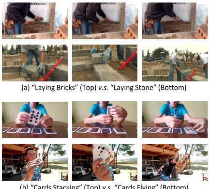
Action recognition in videos has received significant re-search attention in the computer vision and machine learning community (Karpathy et al. 2014; Wang and Schmid 2013; Wang, Qiao, and Tang 2016; Simonyan and Zisserman 2014; Fernando et al. 2015; Wang et al. 2016; Qiu, Yao, and Mei 2017; Carreira and Zisserman 2017; Shi et al. 2017; Zhang et al. 2016). The increasing ubiquity of recording de-vices has created videos far surpassing what we can man-ually handle. It is therefore desirable to develop automatic video understanding algorithms for various applications, such as video recommendation, human behavior analysis, video surveillance and so on. Both local and global infor-mation is important for this task, as shown in Fig.1. For ex-ample, to recognize “Laying Bricks” and “Laying Stones”, local spatial information is critical to distinguish bricks and stones; and to classify “Cards Stacking” and “Cards Flying”, global spatial-temporal clues are the key evidence.

Copyright c2019, Association for the Advancement of Artificial Intelligence (www.aaai.org). All rights reserved.

(a) “Laying Bricks” (Top) v.s. “Laying Stone” (Bottom)

(b) “Cards Stacking” (Top) v.s. “Cards Flying” (Bottom)

Figure 1: Local information is sufficient to distinguish “Laying Bricks” and “Laying Stones” while global spatial-temporal clue is necessary to tell “Cards Stacking” and “Cards Flying”.

Motivated by the promising results of deep networks (Ioffe and Szegedy 2015; He et al. 2016; Szegedy et al. 2017) on image understanding tasks, deep learning is ap-plied to the problem of video understanding. Two major re-search directions are explored specifically for action recog-nition, i.e., employing CNN+RNN architectures for video sequence modeling (Donahue et al. 2015; Yue-Hei Ng et al. 2015) and purely deploying ConvNet-based architectures for video recognition (Simonyan and Zisserman 2014; Feicht-enhofer, Pinz, and Wildes 2016; 2017; Wang et al. 2016; Tran et al. 2015; Carreira and Zisserman 2017; Qiu, Yao, and Mei 2017).

the feed-forward CNN part is used for spatial modeling, while the temporal modeling part, i.e., LSTM (Hochreiter and Schmidhuber 1997) or GRU (Cho et al. 2014), makes end-to-end optimization very difficult due to its recurrent ar-chitecture. Nevertheless, separately training CNN and RNN parts is not optimal for integrated spatial-temporal represen-tation learning.

ConvNets for action recognition can be generally cate-gorized into 2D ConvNet and 3D ConvNet. 2D convolu-tion architectures (Simonyan and Zisserman 2014; Wang et al. 2016) extract appearance features from sampled RGB frames, which only exploit local spatial information rather than local spatial-temporal information. As for the tempo-ral dynamics, they simply fuse the classification scores ob-tained from several snippets. Although averaging classifi-cation scores of several snippets is straightforward and ef-ficient, it is probably less effective for capturing spatio-temporal information. C3D (Tran et al. 2015) and I3D (Car-reira and Zisserman 2017) are typical 3D convolution based methods which simultaneously model spatial and temporal structure and achieve satisfying recognition performance. As we know, compared to deeper network, shallow network exhibits inferior capacity on learning representation from large scale datasets. When it comes to large scale human action recognition, on one hand, inflating shallow 2D Con-vNets to their 3D counterparts may be not capable enough of generating discriminative video descriptors; on the other hand, 3D versions of deep 2D ConvNets will result in too big model as well as too heavy computation cost both in training and inference phases.

Given the aforementioned concerns, we propose our novel spatial-temporal network (StNet) to tackle the large scale ac-tion recogniac-tion problem. First, we consider local spatial-temporal relationship by applying 2D convolution on 3N-channel super-image, which is composed of N successive video frames. Thus local spatial-temporal information can be more efficiently encoded compared to 3D convolution on N images. Second, StNet inserts temporal convolutions upon feature maps of super-images to capture temporal relation-ship among them. Local spatial-temporal modeling followed by temporal convolution can progressively builds global spatial-temporal relationship and is lightweight and com-putational friendly. Third, in StNet, the temporal dynamics are further encoded with our proposed temporal Xception block (TXB) instead of averaging scores of several snip-pets. Inspired by separable depth-wise convolution (Chol-let 2017), TXB encodes temporal dynamics in a separate channel-wise and temporal-wise 1D convolution manner for smaller model size and higher computation efficiency. Fi-nally, TXB is convolution based rather than recurrent archi-tecture, it is easily to be optimized via stochastic gradient decent (SGD) in an end-to-end manner.

We evaluate the proposed StNet framework over the newly released large scale action recognition dataset Kinet-ics (Kay et al. 2017). Experiment results show that StNet outperforms several state-of-the-art 2D and 3D convolution based solutions, meanwhile our StNet attains better effi-ciency from the perspective of the number of FLOPs and higher effectiveness in terms of recognition accuracy than

its 3D CNN counterparts. Besides, the learned representa-tion of StNet is transferred to the UCF101 (Soomro, Zamir, and Shah 2012) dataset to verify its generalization capabil-ity.

2

Related Work

In the literature, video-based action recognition solutions can be divided into two categories: action recognition with hand-crafted features and action recognition with deep Con-vNet. To develop effective spatial-temporal representations, researchers have proposed many hand-crafted features such as HOG3D (Klaser, Marszałek, and Schmid 2008), SIFT3D (Scovanner, Ali, and Shah 2007), MBH (Dalal, Triggs, and Schmid 2006). Currently, improved dense trajectory (Wang and Schmid 2013) is the state-of-the-art among the crafted features. Despite its good performance, such hand-crafted feature is designed for local spatial-temporal descrip-tion and is hard to capture semantic level concepts. Thanks to the big progress made by introducing deep convolution neural network, ConvNet based action recognition meth-ods have achieved superior accuracy to conventional hand-crafted methods. As for utilizing CNN for video-based ac-tion recogniac-tion, there exist the following two research di-rections:

Encoding CNN Features:CNN is usually used to extract spatial features from video frames, and the extracted feature sequence is then modelled with recurrent neural networks or feature encoding methods. In LRCN (Donahue et al. 2015), CNN features of video frames are fed into LSTM network for action classification. ShuttleNet (Shi et al. 2017) intro-duced biologically-inspired feedback connections to model long-term dependencies of spatial CNN descriptors. TLE (Diba, Sharma, and Van Gool 2017) proposed temporal lin-ear encoding that captures the interactions between video segments, and encoded the interactions into a compact rep-resentations. Similarly, VLAD (Arandjelovic et al. 2016; Girdhar et al. 2017) and AttentionClusters (Long et al. 2018) have been proposed for local feature integration.

ConvNet as Recognizer: the first attempt to use deep convolution network for action recognition was made by Karpathy et.al, (Karpathy et al. 2014). While strong results for action recognition have been achieved by (Karpathy et al. 2014), two stream ConvNet (Simonyan and Zisserman 2014) that merges the predicted scores from a RGB based spatial stream and an optical flow based temporal stream obtained performance improvements in a large margin. ST-ResNet (Feichtenhofer, Pinz, and Wildes 2016) introduced residual connections between the two streams of (Simonyan and Zisserman 2014) and showed great advantage in results. To model the long-range temporal structure of videos, Tem-poral Segment Network (TSN) (Wang et al. 2016) was pro-posed to enable efficient video-level supervision by sparse temporal sampling strategy and further boosted the perfor-mance of ConvNet based action recognizer.

R

es2

C

onv1

R

es3

R

es4

Re

s5

C

onv_3d

(

, (3,

1,

1),

1)

B

N_3d

R

esha

pe

R

esha

pe

A

vg

P

ool

T

em

pora

l

M

od

ell

in

g

B

lock

T

em

p

or

al

M

odellin

g

B

lock

R

eL

U

…

…

…

…

T

em

p

or

al

Xc

ep

tion

B

lock

R

esha

pe

FC

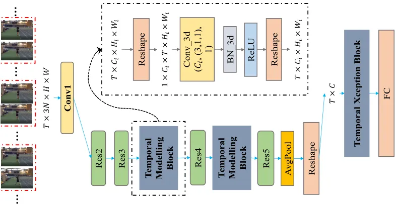
Figure 2: Illustration of constructing StNet based on ResNet (He et al. 2016) backbone. The input to StNet is aT×3N×H×W

tensor. Local spatial-temporal patterns are modelled via 2D Convolution. 3D convolutions are inserted right after the Res3 and Res4 blocks for long term temporal dynamics modelling. The setting of 3D convolution (# Output Channel, (temporal kernel size, height kernel size, width kernel size), # groups) is (Ci, (3,1,1), 1).

to learn spatial-temporal features. Compared to 2D Con-vNets, C3D has more parameters and is much more dif-ficult to obtain good convergence. To overcome this diffi-culty, T-ResNet (Feichtenhofer, Pinz, and Wildes 2017) in-jects temporal shortcut connections between the layers of spatial ConvNets to get rid of 3D convolution. I3D (Carreira and Zisserman 2017) simultaneously learns spatial-temporal representation from video by inflating conventional 2D Con-vNet architecture into 3D ConCon-vNet. P3D (Qiu, Yao, and Mei 2017) decouples a 3D convolution filter to a 2D spatial con-volution filter followed by a 1D temporal concon-volution fil-ter. Recently, there are many frameworks proposed to im-prove 3D convolution (Zolfaghari, Singh, and Brox 2018; Wang et al. 2018a; Xie et al. 2018; Tran et al. 2018; Wang et al. 2018b; Chen et al. 2018). Our work is different in that spatial-temporal relationship is progressively mod-eled via temporal convolution upon local spatial-temporal feature maps.

3

Proposed Approach

The proposed StNet can be constructed from the existing state-of-the-art 2D ConvNet frameworks, such as ResNet (He et al. 2016), InceptionResnet (Szegedy et al. 2017) and so on. Taking ResNet as an example, Fig.2 illustrates how we can build StNet from the existing 2D ConvNet. It is sim-ilar to build StNet from other 2D ConvNet frameworks such as InceptionResnetV2 (Szegedy et al. 2017), ResNeXt (Xie et al. 2017) and SENet (Hu, Shen, and Sun 2018). Therefore, we do not elaborate all such details here.

Super-Image: Inspired by TSN (Wang et al. 2016), we choose to model long range temporal dynamics by sampling temporal snippets rather than inputting the whole video

se-quence. One of the differences from TSN is that we sam-pleT temporal segments each of which consists ofN con-secutive RGB frames rather than a single frame. TheseN

frames are stacked in the channel dimension to form a su-per image, so the input to the network is a tensor of size

T×3N×H×W. Super-Image contains not only local spa-tial appearance information represented by individual frame but also local temporal dependency among these successive video frames. In order to jointly modeling the local spatial-temporal relationship therein and as well as to save model weights and computation costs, we leverage 2D convolution (whose input channel size is 3N) on each of theT super-images. Specifically, the local spatial-temporal correlation is modeled by 2D convolutional kernels inside the Conv1, Res2, and Res3 blocks of ResNet as shown in Fig.2. In our current setting,N is set to 5. In the training phase, 2D con-volution blocks can be initialized directly with weights from the ImageNet pre-trained backbone 2D convolution model except the first convolution layer. Weights of Conv1 can be initialized following what the authors have done in I3D (Car-reira and Zisserman 2017).

Temporal Modeling Block: 2D convolution on the T

BN _1 d Co nv _1 d (C in ,3 ,1 ,C in ) Co nv _1 d (C ou t ,1 ,0 ,1 ) BN _1 d R eL U Co nv _1 d (C ou t ,3 ,1 ,C ou t ) Co nv _1 d (C ou t ,1 ,0 ,1 ) Co nv _1 d (C ou t ,1 ,0 ,1 ) BN _1 d R eL U T×Cin M ax P oo lin g 1×Cout

(a) Temporal Xception block configuration

Channel: Ci

Te

mp

or

al:

T

Conv_1d(Ci,3,1,Ci) Conv_1d(Co,1,0,1)

Ci

T

Co

T

CK1 CKCi

Apply kernel CKj on the j-th Channel

Apply kernel TKj

on each temporal feature TK1 TKCo Fe atu re s K er ne ls CKj TKj

(b) Channel- and temporal-wise convolution

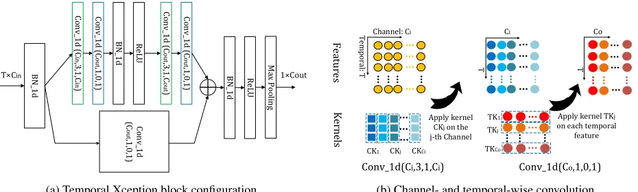
Figure 3: Temporal Xception block (TXB). The detailed configuration of our proposed temporal Xception block is shown in (a). The parameters in the bracket denotes (#kernel, kernel size, padding, #groups) configuration of 1D convolution. Blocks in green denote channel-wise 1D convolutions and blocks in blue denote temporal-wise 1D convolutions. (b) depicts the channel-wise and temporal-wise 1D convolution. Input to TXB is feature sequence of a video, which is denoted as aT ×Cintensor. Every

kernel of channel-wise 1D convolution is applied along the temporal dimension within only one channel. Temporal-wise 1D convolution kernel convolves across all the channels along every temporal step.

so we set both spatial kernel size of a 3D convolution as 1 to save computation cost while the temporal kernel size is empirically set to be 3. Applying 2 temporal convolutions on theT local spatial-temporal feature maps after Res3 and Res4 blocks introduces very limited extra computation cost but is effective to capture global spatial-temporal correlation progressively. In the temporal modeling blocks, weights of Conv3d layers are initially set to1/(3×Ci), whereCi

de-notes input channel size, and biases are set to 0. BN3d is initialized to be an identity mapping.

Temporal Xception Block: Our temporal Xception block is designed for efficient temporal modeling among feature sequence and easy optimization in an end-to-end manner. We choose temporal convolution to capture temporal rela-tions instead of recurrent architectures mainly for the end-to-end training purpose. Unlike ordinary 1D convolution which captures the channel-wise and temporal-wise information jointly, we decouple channel-wise and temporal-wise calcu-lation for computational efficiency.

The temporal Xception architecture is shown in Fig.3(a). The feature sequence is viewed as aT×Cintensor, which is

obtained by globally average pooling from the feature maps ofTsuper-images. Then, 1D batch normalization (Ioffe and Szegedy 2015) along the channel dimension is applied to such an input to handle the well-known co-variance shift is-sue, the output signal isV,

vi =u

i_−m

√

var ∗α+β (1)

wherevi andui denote theithrow of the output and in-put signals, respectively;αandβ are trainable parameters,

mandvar are accumulated running mean and variance of input mini-batches. To model temporal relation, convolu-tions along the temporal dimension are applied toV. We de-couple temporal convolution into separate channel-wise and temporal-wise 1D convolutions. Technically, for channel-wise 1D convolution, the temporal kernel size is set to 3,

and the number of kernels and the group number are set to be the same with the input channel number. In this sense, ev-ery kernel convolves over temporal dimension within a sin-gle channel. For temporal-wise 1D convolution, we set both the kernel size and the group number to 1, so that temporal-wise convolution kernels operate across all elements along the channel dimension at each time step. Formally, channel-wise and temporal-channel-wise convolution can be described with Eq.2 and Eq.3, respectively,

yi,j=

2 X

k=0

xk+i−1,j∗W

(c)

j,k,0+b

(c)

j , (2)

yi,j =

Ci

X

k=0

xi,k∗W

(t)

j,0,k+b

(t)

j , (3)

wherex ∈ RT×Ci _{is the inputC}

i-Dimfeature sequence

of length T,y ∈ RT×Co _{denotes output feature sequence} and yi,j is the value of the jth channel of the ith

fea-ture, ∗ denotes multiplication. In Eq.2,W(c) _{∈ R}Co×3×1 denotes the channel-wise Conv kernel of (#kernel, kernel size, #groups) = (Co,3,Ci). In Eq.3,W(t)∈RCo×1×Ci

de-notes the temporal-wise Conv kernel of (#kernel, kernel size, #groups) = (Co,1,1).bdenotes bias. In this paper,Cois set

to 1024. An intuitive illustration of separate channel- and temporal-wise convolution can be found in Fig.3(b).

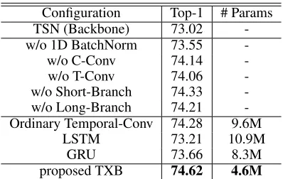
Configuration Top-1 # Params TSN (Backbone) 73.02 -w/o 1D BatchNorm 73.55

-w/o C-Conv 74.14

-w/o T-Conv 74.06

-w/o Short-Branch 74.33 -w/o Long-Branch 74.21 -Ordinary Temporal-Conv 74.28 9.6M

LSTM 73.21 10.9M

GRU 73.66 8.3M

proposed TXB 74.62 4.6M

Table 1: Ablation study of TXN on Kinetics400. C-Conv and T-Conv denote channel-wise and temporal-wise 1D Conv, respectively. Prec@1 and number of model parameters are reported in the table.

the temporal Xception block is fed into a 1D max-pooling layer along the temporal dimension, and the pooled output is used as the spatial-temporal aggregated descriptor for clas-sification.

4

Experiments

4.1

Datasets and Evaluation Metric

To evaluate the performance of our proposed StNet frame-work for large scale video-based action recognition, we per-form extensive experiments on the recent large scale action recognition dataset named Kinetics (Kay et al. 2017). The first version of this dataset (denoted as Kinetics400) has 400 human action classes, with more than 400 clips for each class. The validation set of Kinetics400 consists of about 20K video clips. The second version of Kinetics (denoted as Kinetics600) contains 600 action categories and there are about 400K trimmed video clips in its training set and 30K clips in the validation set. Due to unavailability of ground truth annotations for testing set, the results on the Kinetics dataset in this paper are evaluated on its validation set.

To validate that the effectiveness of StNet could be trans-ferred to other datasets, we conduct transfer learning exper-iments on the UCF101 (Soomro, Zamir, and Shah 2012), which is much smaller than Kinetics. It contains 101 hu-man action categories and 13,320 labeled video clips in total. The labeled video clips are divided into three training/testing splits for evaluation. In this paper, the evaluation metric for recognition effectiveness is average class accuracy, we also report total number of model parameters as well as FLOPs (total number of float-point multiplications executed in the inference phase) to depict model complexity.

4.2

Ablation Study

Temporal Xception Block: We conduct ablation experi-ments on our proposed temporal Xception block. To show the contribution of each component in TXB, we disable each of them one by one, and then train and test the models on the RGB feature sequence, which is extracted from the GlobalAvgPool layer of InceptionResnet-V2-TSN (Wang et

Configurations

Top-1 Super-Image TM Blocks TXB

× (N=1) × × 72.2

√

(N=5) × × 74.2

√

(N=5) √ × 76.0

√

(N=5) √ √ 76.3

Table 2: Results evaluated on Kinetics600 validation set with different network configurations andT = 7.

al. 2016) model trained on the Kinetics400 dataset. Be-sides, we also implemented an ordinary 2-layered tempo-ral Conv model (denoted as Ordinary Tempotempo-ral-Conv) and RNN-based models (LSTM (Hochreiter and Schmidhuber 1997) and GRU (Cho et al. 2014)) for comparison. In Ordi-nary Temporal-Conv model, we replace the temporal Xcep-tion module by two 1D convoluXcep-tion layers, whose kernel size is 3 and output channel number is 1024, to temporally model the input feature sequence. In this experiment, the hidden units of LSTM and GRU is set to 1024. The final classifi-cation results are predicted by a fully connected layer with output size of 400. For each video, features of 25 frames are evenly sampled from the whole feature sequence to train and test all the models. The evaluation results and number of parameters of these models are reported in Table.1

From the top lines of Table.1, we can see that each com-ponent contributes to the proposed TXB framework. Batch normalization handles the co-variance shift issue and it brings 1.07% absolute top-1 accuracy improvement for RGB stream. Separate channel-wise and temporal-wise convolu-tion layers is helpful for modeling temporal relaconvolu-tions, and recognition performance drops without either of them. The results also demonstrate that our design of long-branch plus short-branch is useful by mixing multiple temporal receptive field encodings. Comparing the results listed in the middle lines with that of our TXB, it is clear that TXB achieves the best top-1 accuracy among these models and the model is the smallest (with only 4.6 million parameters in total), es-pecially, the gain over backbone TSN is up to 1.6 percent.

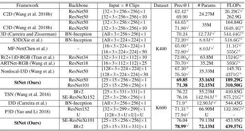
Framework Backbone Input×# Clips Dataset Prec@1 # Params FLOPs

C2D (Wang et al. 2018b) ResNet50 [32×3×256×256]×1

K400

62.42×

24.27M 26.29G √

ResNet50 [32×3×256×256]×10 69.90 262.9G

C3D (Wang et al. 2018b)

ResNet50 [32×3×256×256]×1 64.65×

35M 164.84G ResNet50 [32×3×256×256]×10 71.86√ 1648.4G×

I3D (Carreira and Zisserman) BN-Inception [All×3×256×256]×1 70.24 12.7M√ 544.44G×

S3D(Xie et al.) BN-Inception [All×3×224×224]×1 72.20√ 8.8M√ 518.6G×

MF-Net(Chen et al.) - [16×3×224×224]×1 65.00

×

8.0M

√ _11.1G√

[16×3×224×224]×50 72.80√ 555G×

R(2+1)D-RGB (Tran et al.) ResNet34 [32×3×112×112]×10 72.00√ 63.8M 1524G×

ARTNet-RGB (Wang et al.) ResNet18 [16×3×112×112]×25 70.70√ 35.2M 593G×

Nonlocal-I3D (Wang et al.) ResNet50 [128×3×224×224]×1 67.30 ×

35.33M 145.7G

[128×3×224×224]×30 76.50√ 4371G×

StNet (Ours) ResNet50 [25×15×256×256]×1 69.85 33.16M 189.29G ResNet101 [25×15×256×256]×1 71.38 52.15M 310.50G

TSN (Wang et al. 2016) IRv2 [25×3×331×331]×1

K600

76.22 55.23M 410.85G SE-ResNeXt152 [25×3×256×256]×1 76.16 142.94M× 875.21G×

I3D (Carreira et al.) BN-Inception [All×3×256×256]×1 71.9× 12.90M√ 544.45G

P3D (Yao and Li 2018) ResNet152 [32×3×299×299]×1 71.31

× _{66.90M 132.38G}√

U [128×3×U×U]×U 77.94√ U

-StNet (Ours) SE-ResNeXt101 [25×15×256×256]×1 76.04 79.13M 453.95G

IRv2 [25×15×331×331]×1 78.99

√

72.13M 439.57G

Table 3: Comparison of StNet and several state-of-the-art 2D/3D convolution based solutions. The results are reported on validation set of Kinetics400 and Kinetics600, with RGB modality only. We investigate both Prec@1 and model efficiency w.r.t. total number of model parameters and FLOPs in inference. Here, “IRv2” denotes InceptionResNet-V2, “K400” is short for Kinetics400 and so is the case for “K600”. U denotes unknown. “All” means using all frames in a video.

Experiment results are reported in Table.2. When the three components are all disabled, the model degrades to be TSN (Wang et al. 2016), which achieves top-1 precision of 72.2% on Kinetics600 validation set. By enabling super-image, the recognition performance is improved by 2.0% and the gain comes from introducing local spatial-temporal modelling. When the two temporal modelling blocks are inserted, the Prec@1 is further boosted to 76.0%, it evidences the fact that modeling global spatial-temporal interactions among the feature maps of super-images is necessary for perfor-mance improvement, because it can well represent high-level video features. The final performance is 76.3% when all the components are integrated and this shows that us-ing TXB to capture long-term temporal dynamics is still a plus even if local and global spatial-temporal relationship is modeled by enabling super-images and temporal modeling blocks.

4.3

Comparison with Other Methods

We evaluate the proposed framework against the recent state-of-the-art 2D/3D convolution based solutions. Exten-sive experiments are conducted on the datasets of Kinet-ics400 and Kinetics600 to make comparisons among these models in terms of their effectiveness (i.e., top-1 accuracy) and efficiency (reflected by total number of model param-eters and FLOPs needed in the inference phase). To make thorough comparison, we evaluated different methods with several relatively small backbone networks and a few very

deep backbones on Kinetics400 and Kinetics600, respec-tively. Results are summarized in Table.3. Numbers with

√

mean that the results are pleasing and numbers with× repre-sent unsatisfying ones. From the evaluation results, we can draw the following conclusions:

StNet outperforms 2D-Conv based solution:(1) C2D-ResNet50 is cheap in FLOPs, but its top-1 recognition preci-sion is very poor (62.42%) if only 1 clip is tested. When 10 clips are tested, the performance is boosted to 69.9% at the cost of 262.9G FLOPs. StNet-ResNet50 achieves Prec@1 of 69.85% and only 189.29G FLOPs are needed. (2) When large backbone models are used, StNet still outperforms 2D-Conv based solution, this can be concluded from the fact that StNet-IRv2 significantly boosts the performance of TSN-IRv2 (which is 76.22%) to 78.99% while the total number of FLOPs is slightly increased from 410.85G to 439.57G. Besides, StNet-SE-ResNeXt101 performs comparable with TSN-SE-ResNeXt152, but the model size and FLOPs are significantly saved (from 875.21G to 453.95G).

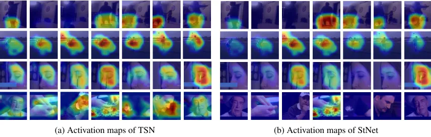
P3D-(a) Activation maps of TSN (b) Activation maps of StNet

Figure 4: Visualizing action-specific activation maps with the CAM (Zhou et al. 2016). Four action classes, i.e., hoverboarding, golf driving ,filling eyebrows and playing poker, are shown from top to the bottom. It is clear that StNet can well capture temporal dynamics in video and focuses on the spatial-temporal regions which really corresponds to the action class.

ResNet152, StNet-IRv2 outperforms by a large margin (78.99% v.s. 71.31) with acceptable FLOPs increase (from 132.38G to 439.57G). Besides, Single clip test performance of StNet-IRv2 still outperforms P3D by 1.05%, which is used for the Kinetics600 challenge with 128 frames input and no further details about its backbone, input size as well as number of testing clips. (3) Compared with S3D (Xie et al. 2018), R(2+1)D(Tran et al. 2018), MF-Net (Chen et al. 2018) and Nonlocal-I3d (Wang et al. 2018b), the proposed StNet can still strike good performance-FLOPs trade-off.

4.4

Transfer Learning on UCF101

We transfer RGB models of StNet pre-trained on Kinetics to the much smaller dataset of UCF101 (Soomro, Zamir, and Shah 2012) to show that the learned representation can be well generalized to other dataset. The results included in Ta-ble 4 are the mean class accuracy from three training/testing splits. It is clear that our Kinetics pre-trained StNet models with ResNet50, ResNet101 and the large InceptionResNet-V2 backbone demonstrate very powerful transfer learning capability, and mean class accuracy is up to 93.5%, 94.3% and 95.7%, respectively. Specifically, the transferred StNet-IRv2 RGB model achieves the state-of-the-art performance while its FLOPs is 123G.

Model Pre-Train FLOPs Accuracy

C3D+Res18 K400 - 89.8

I3D+BNInception K400 544G× _95.6 TSN+BNInception K400 - 91.1 TSN+IRv2 (T=25) K400 411G 92.7 StNet-Res50 (T=7) K400 53G

√

93.5 StNet+Res101 (T=7) K400 87G 94.3 StNet+IRv2 (T=7) K600 123G 95.7

√

Table 4: Mean class accuracy of different models transferred on UCF101. RGB frames of UCF101 are used for training and testing. The mean class accuracy averaged over the three splits of UCF101 is reported.

4.5

Visualization in StNet

To help us better understand how StNet learns discriminative spatial-temporal descriptors for action recognition, we visu-alize the class-specific activation maps of our model with the CAM (Zhou et al. 2016) approach. In this experiment, we setT to 7 and the 7 snippets are evenly sampled from video sequences in the Kinetics600 validation set to obtain their class-specific activation map. As a comparison, we also visualize the activation maps of TSN model, which exploits local spatial information and then fusesT snippets by aver-aging classification score rather than jointly modeling local and global spatial-temporal information. As an illustration, Fig. 4 lists activation maps of four action classes (hover-boarding, golf driving, filling eyebrows and playing poker) of both models.

These maps shows that, compared to TSN which fails to jointly model local and global spatial-temporal dynamics in videos, our StNet can capture the temporal interactions in-side video frames. It focuses on the spatial-temporal regions which are closely related to the groundtruth action. For ex-ample, it pays more attention to faces with eyebrow pencil in the nearby while regions with only faces are not so ac-tivated. Particularly, in the “play poker” example, StNet is significantly activated only by the hands and casino tokens. Nevertheless, TSN is activated by many regions of faces.

5

Conclusion

scale dataset and boosting the final action recognition accu-racy. Extensive experiments on large scale action recogni-tion benchmark Kinetics have verified the effectiveness of StNet. In addition, StNet trained on Kinetics exhibits pretty good transfer learning ability on the UCF101 dataset.

References

Arandjelovic, R.; Gronat, P.; Torii, A.; Pajdla, T.; and Sivic, J. 2016. Netvlad: Cnn architecture for weakly supervised place recognition. InCVPR, 5297–5307.

Carreira, J., and Zisserman, A. 2017. Quo vadis, action recogni-tion? a new model and the kinetics dataset. InCVPR, 4724–4733. Carreira, J.; Noland, E.; Banki-Horvath, A.; Hillier, C.; and Zisser-man, A. 2018. A short note about kinetics-600. arXiv preprint arXiv:1808.01340.

Chen, Y.; Kalantidis, Y.; Li, J.; Yan, S.; and Feng, J. 2018. Multi-fiber networks for video recognition. InECCV, 352–367. Cho, K.; Van Merri¨enboer, B.; Bahdanau, D.; and Bengio, Y. 2014. On the properties of neural machine translation: Encoder-decoder approaches.arXiv preprint arXiv:1409.1259.

Chollet, F. 2017. Xception: Deep learning with depthwise separa-ble convolutions. InCVPR, 1800–1807.

Dalal, N.; Triggs, B.; and Schmid, C. 2006. Human detection using oriented histograms of flow and appearance. InECCV, 428–441. Springer.

Diba, A.; Sharma, V.; and Van Gool, L. 2017. Deep temporal linear encoding networks. InCVPR, 1541–1550.

Donahue, J.; Anne Hendricks, L.; Guadarrama, S.; Rohrbach, M.; Venugopalan, S.; Saenko, K.; and Darrell, T. 2015. Long-term re-current convolutional networks for visual recognition and descrip-tion. InCVPR, 2625–2634.

Feichtenhofer, C.; Pinz, A.; and Wildes, R. 2016. Spatiotemporal residual networks for video action recognition. InNIPS, 3468– 3476.

Feichtenhofer, C.; Pinz, A.; and Wildes, R. P. 2017. Temporal residual networks for dynamic scene recognition. InCVPR, 4728– 4737.

Fernando, B.; Gavves, E.; Oramas, J. M.; Ghodrati, A.; and Tuyte-laars, T. 2015. Modeling video evolution for action recognition. In

CVPR, 5378–5387.

Girdhar, R.; Ramanan, D.; Gupta, A.; Sivic, J.; and Russell, B. 2017. Actionvlad: Learning spatio-temporal aggregation for action classification. InCVPR, 3165–3174.

He, K.; Zhang, X.; Ren, S.; and Sun, J. 2016. Deep residual learn-ing for image recognition. InCVPR, 770–778.

Hochreiter, S., and Schmidhuber, J. 1997. Long short-term mem-ory.Neural computation9(8):1735–1780.

Hu, J.; Shen, L.; and Sun, G. 2018. Squeeze-and-excitation net-works. InCVPR, 7132–7141.

Ioffe, S., and Szegedy, C. 2015. Batch normalization: Accelerat-ing deep network trainAccelerat-ing by reducAccelerat-ing internal covariate shift. In

ICML, 448–456.

Karpathy, A.; Toderici, G.; Shetty, S.; Leung, T.; Sukthankar, R.; and Fei-Fei, L. 2014. Large-scale video classification with convo-lutional neural networks. InCVPR, 1725–1732.

Kay, W.; Carreira, J.; Simonyan, K.; Zhang, B.; Hillier, C.; Vijaya-narasimhan, S.; Viola, F.; Green, T.; Back, T.; Natsev, P.; et al. 2017. The kinetics human action video dataset. arXiv preprint arXiv:1705.06950.

Klaser, A.; Marszałek, M.; and Schmid, C. 2008. A spatio-temporal descriptor based on 3d-gradients. InBMVC, 1–10. Long, X.; Gan, C.; de Melo, G.; Wu, J.; Liu, X.; and Wen, S. 2018. Attention clusters: Purely attention based local feature integration for video classification. InCVPR, 7834–7843.

Qiu, Z.; Yao, T.; and Mei, T. 2017. Learning spatio-temporal repre-sentation with pseudo-3d residual networks. InICCV, 5534–5542. IEEE.

Scovanner, P.; Ali, S.; and Shah, M. 2007. A 3-dimensional sift descriptor and its application to action recognition. InACM MM, 357–360.

Shi, Y.; Tian, Y.; Wang, Y.; Zeng, W.; and Huang, T. 2017. Learning long-term dependencies for action recognition with a biologically-inspired deep network. InICCV, 716–725.

Simonyan, K., and Zisserman, A. 2014. Two-stream convolutional networks for action recognition in videos. InNIPS, 568–576. Soomro, K.; Zamir, A. R.; and Shah, M. 2012. Ucf101: A dataset of 101 human actions classes from videos in the wild.arXiv preprint arXiv:1212.0402.

Szegedy, C.; Ioffe, S.; Vanhoucke, V.; and Alemi, A. A. 2017. Inception-v4, inception-resnet and the impact of residual connec-tions on learning. InAAAI, 4278–4284.

Tran, D.; Bourdev, L.; Fergus, R.; Torresani, L.; and Paluri, M. 2015. Learning spatiotemporal features with 3d convolutional net-works. InICCV, 4489–4497.

Tran, D.; Wang, H.; Torresani, L.; Ray, J.; LeCun, Y.; and Paluri, M. 2018. A closer look at spatiotemporal convolutions for action recognition. InCVPR, 6450–6459.

Wang, H., and Schmid, C. 2013. Action recognition with improved trajectories. InICCV, 3551–3558.

Wang, L.; Xiong, Y.; Wang, Z.; Qiao, Y.; Lin, D.; Tang, X.; and Van Gool, L. 2016. Temporal segment networks: Towards good practices for deep action recognition. InECCV, 20–36.

Wang, L.; Li, W.; Li, W.; and Van Gool, L. 2018a. Appearance-and-relation networks for video classification. InCVPR, 1430–1439. Wang, X.; Girshick, R.; Gupta, A.; and He, K. 2018b. Non-local neural networks. InCVPR, 7794–7803.

Wang, L.; Qiao, Y.; and Tang, X. 2016. MoFAP: A multi-level rep-resentation for action recognition. International Journal of Com-puter Vision119(3):254–271.

Xie, S.; Girshick, R.; Doll´ar, P.; Tu, Z.; and He, K. 2017. Aggre-gated residual transformations for deep neural networks. InCVPR, 5987–5995.

Xie, S.; Sun, C.; Huang, J.; Tu, Z.; and Murphy, K. 2018. Rethink-ing spatiotemporal feature learnRethink-ing: Speed-accuracy trade-offs in video classification. InECCV, 305–321.

Yao, T., and Li, X. 2018. Yh technologies at activitynet challenge 2018.arXiv preprint arXiv:1807.00686.

Yue-Hei Ng, J.; Hausknecht, M.; Vijayanarasimhan, S.; Vinyals, O.; Monga, R.; and Toderici, G. 2015. Beyond short snippets: Deep networks for video classification. InCVPR, 4694–4702. Zhang, B.; Wang, L.; Wang, Z.; Qiao, Y.; and Wang, H. 2016. Real-time action recognition with enhanced motion vector CNNs. InCVPR, 2718–2726.

Zhou, B.; Khosla, A.; Lapedriza, A.; Oliva, A.; and Torralba, A. 2016. Learning deep features for discriminative localization. In

CVPR, 2921–2929.