DOI: 10.1534/genetics.105.042978
Modeling Haplotype Block Variation Using Markov Chains
G. Greenspan
1and D. Geiger
Computer Science Department, Technion, Haifa 32000, Israel Manuscript received March 7, 2005
Accepted for publication November 23, 2005
ABSTRACT
Models of background variation in genomic regions form the basis of linkage disequilibrium mapping methods. In this work we analyze a background model that groups SNPs into haplotype blocks and represents the dependencies between blocks by a Markov chain. We develop an error measure to compare the perfor-mance of this model against the common model that assumes that blocks are independent. By examining data from the International Haplotype Mapping project, we show how the Markov model over haplotype blocks is most accurate when representing blocks in strong linkage disequilibrium. This contrasts with the independent model, which is rendered less accurate by linkage disequilibrium. We provide a theoretical explanation for this surprising property of the Markov model and relate its behavior to allele diversity.
G
ENETIC mapping studies based on linkagedis-equilibrium (LD) require a model of the back-ground variation in the region being examined. The studies look for markers at which the norms of this model are violated by a set of diseased individuals, in-ferring that any such markers are likely to be close to a disease-causing allele. While many LD mapping meth-ods do not explicitly refer to such a background model, it exists nonetheless as an underlying assumption. For
example, ax2-correlation test between disease status and
the allele frequencies at individual SNPs assumes that the alleles at each SNP are distributed independently. Recent work on human genomic variation suggests that it is fruitful to group SNP markers together into
hap-lotype blocks (Dalyet al.2001; Goldstein2001; Patil
et al.2001; Gabrielet al.2002; Walland Pritchard 2003). These blocks are thought to be delineated by recombination hotspots, small areas in which the prob-ability of recombination is far higher than that in
the surrounding regions ( Jeffreys et al. 2000, 2001;
Templetonet al.2000; Wanget al.2002; Arnheimet al.
2003; Phillipset al.2003; Twellset al.2003). The low
probability of recombination inside each block means that the alleles at the SNPs within are passed together from one generation to the next. Therefore, each hap-lotype block can be considered as a single marker, with the set of alleles at the SNPs in the block constituting
its allele (Cardon and Abecasis2003; Tishkoff and
Verrelli 2003). It is hoped that haplotype blocks will enable fewer SNP markers to be genotyped during LD mapping studies, since a small number of haplotype-tagging SNPs (htSNPs) can be used to identify the
common alleles of each block ( Johnson et al. 2001;
Zhanget al.2002; Sebastianiet al.2003). The Interna-tional Haplotype Mapping Project (HapMap) is currently producing a high-density haplotype map of the human genome for several target populations, to enable the
efficient selection of htSNPs (International HapMap
Consortium2003).
It is not practical or desirable to represent the back-ground variation over SNP or block markers in a large chromosomal region using a full joint distribution. A model must also infer something about the structure of the distribution, so that it is sufficiently robust to deal with additional individuals or a future generation. Since models of background variation are generally inferred from a small sample of haplotypes, many haplotypes present in the population will not appear in the sample obtained.
The most obvious approximation of the full joint distribution is a model that assumes that all markers are
independent,i.e., that the probability of a haplotype is
the product of the frequencies of each allele within. This type of model is common and constitutes an im-plicit assumption in many LD mapping studies. The independent model has the advantage of requiring a small number of parameters, namely the frequencies for each allele. However, this model breaks down when rep-resenting the variation over short distances, since mark-ers that are close together tend to exhibit a high degree of linkage disequilibrium that cannot be captured by an independent approximation.
In this article, we focus on a different model, namely the Markov chain. In the Markov model, the probability of each allele at a marker is conditional on the allele present at the previous marker. This model is able to represent some of the correlations that exist in a ge-nomic region, while still keeping to a linear number of 1Corresponding author: Computer Science Department, Technion,
Technion City, Haifa 32000, Israel. E-mail: [email protected]
parameters. For example, when modeling block markers with four possible alleles, the Markov model will require four times as many parameters as the independent model. Many of the existing methods for partitioning regions into haplotype blocks include a Markov chain in their
models (Dalyet al.2001; Andersonand Novembre2003;
Greenspan and Geiger 2004a; Kimmel and Shamir 2004). Several published approaches to LD mapping also use a Markov chain to represent the background
variation over blocks or individual SNPs (McPeekand
Strahs1999; Morriset al.2000; Liuet al.2001; Morris et al.2002; Greenspanand Geiger2004b).
For any given joint distribution, a Markov approxima-tion will clearly be more accurate than an independent approximation, since it has more parameters available for optimization. However, we describe in this article an important additional property of the Markov approx-imation that we consider surprising. When used to model haplotype blocks, the Markov approximation is most accurate in the presence of high levels of linkage disequilibrium. Consequently, the Markov model is more accurate for blocks that are close together than for those that are far apart. We also show that when modeling individual SNPs instead of haplotype blocks, this property of the Markov model is not exhibited. In other words, a Markov model over haplotype blocks provides a uniquely accurate way to represent back-ground genomic distributions at high resolution. This result justifies previous work that uses a Markov model over haplotype blocks for both haplotype resolution and
LD mapping (Greenspanand Geiger2004a,b).
MATERIALS AND METHODS
Independent and Markov approximations: Consider a genomic region that contains l markers, placed at physical locationsz1,. . .,zlalong the chromosome (measured in base
pairs). Each markerj¼1,. . .,lhasrjalleles, labeled 1,. . .,rj.
We consider a population in Hardy–Weinberg equilibrium, so the background variation for the region is given in terms of a joint distribution over haplotype frequencies (Hardy1908). LetP(x1,. . .,xl) be the frequency of haplotypex1,. . .,xlin
the population, where eachxjtakes the values 1,. . .,rj.
Under the independent model, each marker is assumed to be independent. The maximum-likelihood independent ap-proximationT(x1,. . .,xl) of the joint distributionPis
Tðx1;. . .;xlÞ ¼ Yl
i¼1
PðxiÞ;
where
PðxiÞ ¼
X
x1;...;xi1;xi11;...;xl
Pðx1;. . .;xlÞ:
Under the Markov model, the distribution for each marker is dependent on the allele present at the preceding marker. The maximum-likelihood Markov approximationQ(x1,. . .,xl)
of the joint distribution is
Qðx1;. . .;xlÞ ¼Pðx1Þ Y l1
i¼1
Pðxi11jxiÞ;
where
Pðxi11jxiÞ ¼ P
x1;...;xi1;xi12;...;xlPðx1;. . .;xlÞ
P
x1;...;xi1;xi11;...;xlPðx1;. . .;xlÞ
:
Error measures:Given a distancedand a numbern$3 of markers, we generate statisticsYd,nand Zd,nto quantify the
average error of the independent and Markov approxima-tions, respectively, over a chromosome or large genomic re-gion. We set a minimum ofn¼3 since a Markov model can represent any joint distribution over one or two loci perfectly, rendering our measure meaningless.
The statisticsYd,nand Zd,nfor a genomic region are
gen-erated by averaging the respective sets of statisticsYd,n(j) and
Zd,n(j) over all valid start markersjwithin that region. Every
value ofYd,nandZd,nin our results was calculated by averaging
hundreds or thousands of these individual measurements. Each statisticYd,n(j) orZd,n(j) measures the error of the
inde-pendent or Markov approximation overnmarkers, where the first markerj1¼jand the other markersj2,. . .,jnare chosen
to be spread approximately evenly over total distanced. Each markerjiis selected to minimizejzjizj1d ði1Þ=ðn1Þj. If any two of the marker indexes j1,. . .,jn are identical,
we conclude that there is insufficient marker density forn,d, andj. In this case,jis not a valid start marker and we omit Yd,n(j) andZd,n(j) from their respective averages.
We setYd;nðjÞ ¼ kPðxj1;. . .;xjnÞ Tðxj1;. . .;xjnÞk, the
var-iation distance between the observed joint distributionPand the independent approximation T for markers j1,. . .,jn.
Similarly, we setZd;nðjÞ ¼ kPðxj1;. . .;xjnÞ Qðxj1;. . .;xjnÞk,
the variation distance betweenPand the Markov approxima-tion Q. The variation distance between two distributions is defined as follows:
kAðz1;. . .;znÞ Bðz1;. . .;znÞk
¼1 2
X
z1;...;zn
jAðz1;. . .;znÞ Bðz1;. . .;znÞj:
This measure is also known as the total variational distance, Kolmogorov distance, orL1distance. It has an intuitive defini-tion as the total amount of probability mass that must be moved to make one distribution equal to the other. For example,kP Tkis the percentage of the population distributed asPthat is misrepresented by the independent approximationT.
The variation distance between the joint distributionPand its independent approximationTis closely related to the D measure of linkage disequilibrium for two biallelic markers. Consider two markers A and B, each with two allelesa1,a2,b1, andb2at frequenciesp1,p2,q1, andq2, respectively. Letp11,p12, p21, andp22be the respective frequencies of the four gametes a1b1,a1b2,a2b1, anda2b2. The linkage disequilibrium measure Dis defined asD¼p11p1q1¼p1q2p12¼p2q1p21¼p22 p2q2(Devlinand Risch1995). For example, if A and B are in perfect linkage equilibrium, thenp11¼p1q1,p12¼p1q2,p21¼ p2q1, andp22¼p2q2, and soD¼0. By comparison, the variation distance betweenPandTis
kPTk ¼1
2ðjp11p1q1j1jp12p1q2j1jp21p2q1j1jp22p2q2jÞ
¼1
2ðjDj1jDj1jDj1jDjÞ ¼2jDj:
HapMap analysis: We used the October 2004 data release of HapMap to profile the error rates of the independent and Markov approximations for the human genome (InternationalHapMap Consortium 2003). We inferred the transmitted and untransmitted haplotypes from both parents in the 30 CEPH trios, so that 120 haplotypes were examined for each of the 22 autosomes. Haplotype alleles that could not be determined were left as unknown. This occurred at sites for which (a) a genotype was absent, (b) a Mendelian error was detected, or (c) all three members of the trio were heterozygous.
We examined the HapMap data using three different ap-proaches: (a) treating each SNP as an individual marker, (b) grouping the SNPs into haplotype blocks according to various criteria, and (c) grouping fixed numbers of adjacent SNPs into arbitrary blocks.
For the first approach, each SNP marker hadrj¼2 alleles,
since all SNP markers genotyped in the HapMap are biallelic. Trivially,zjwas set to the physical location of each SNP.
For the second approach, we used two programs, Haplo-Block and HaploHaplo-BlockFinder, to partition the SNP data for each chromosome intolblocks (Zhangand Jin2003; Greenspan and Geiger2004b). Each block inferred was considered as a marker and the variants of that block as the marker’s alleles. The physical locationzjof each blockjwas set to the midpoint
of the chromosomal section containing the SNPs within. HaploBlock uses a statistical model-fitting criterion to in-fer the most suitable block partition for a genomic region (Greenspanand Geiger2004b). When inferring blocks with HaploBlock, we removed the dependencies between adjacent ancestor variables in the statistical model, to prevent a poten-tial bias in favor of the Markov approximation. We inferred three full HaploBlock models from the HapMap data, with a maximum of four, six, and eight ancestral haplotypes per block, respectively. The HaploBlock statistical model also allows for recent mutations, so some of the haplotypes ob-served in a block might differ slightly from their inferred ancestors.
HaploBlockFinder offers a number of different criteria for inferring block paritions (Zhangand Jin2003). We chose the commonly used chromosomal coverage criterion. This crite-rion defines a block as a region in which a certain percentage of the chromosomes can be covered by four haplotypes, with no additional mutations. We inferred three full HaploBlock-Finder partitions from the HapMap data, with percentage thresholds of 70, 80, and 90%, respectively. As this percentage threshold increases, more of the haplotypes within each block must be covered by four common variants, so less variation is permitted overall.
For the third approach, we grouped sets of up to six ad-jacent SNPs into block markers, without using any additional criterion. The alleles of each marker were defined by the observed combinations of alleles at the SNPs within. The goal of this approach was to determine whether the results ob-served for haplotype blocks are specific to the criteria used or whether similar results are observed for such groupings of SNPs.
Recall that we omit valuesYd,n(j) andZd,n(j) from the
aver-agesYd,nandZd,nifnmarkers are not available with roughly
equal spacing over distance dstarting at markerj. We also omitted the statisticsYd,n(j) andZd,n(j) if less than half of the
120 haplotypes could be used for sites j1,. . .,jn, due to
missing genotypes or haplotype uncertainty. For the SNP ana-lyses, a haplotype could not be used if one of the alleles at sites j1,. . .,jnwas not known. For the block-based analyses, a
hap-lotype could not be used if one of the sets of block alleles could not be assigned to a specific block variant with.50% certainty.
RESULTS
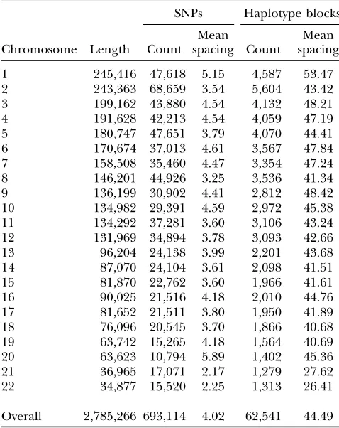
Summary of models: Table 1 summarizes the SNP loci examined for each chromosome, as well as the characteristics of the HaploBlock statistical models inferred with up to four variants per block. Table 1 shows that the average SNP spacing over all 22 chromo-somes is 4.02 kb, whereas the average spacing between the blocks is 44.49 kb. These values provide a rough
lower bound on the distances d and n that can be
examined usefully for the respective models, since n
markers spread over distancedmust be spaced at least
d/(n1) apart to be included in the averagesYd,nand
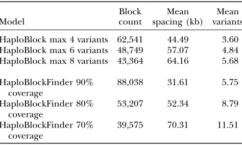
Zd,n. Table 2 compares the average values over all 22
chromosomes for the six HaploBlock and HaploBlock-Finder models. Table 2 also shows the average number of variants inferred per block for each model.
Distance profiles: We assessed how the error rates of the independent and Markov approximations varied
over different distancesd. The distance profiles were
gen-erated by calculating average values ofYd,nandZd,nover
the entire autosome for values of 3#n#5.
We first examine the results for the HaploBlock model with up to four variants per block. Figure 1 shows
the error measuresZd,nfor the Markov approximation
for this model over different distances d. Values are
TABLE 1
Summary for each chromosome of SNPs and the HaploBlock model with up to four variants
SNPs Haplotype blocks
Chromosome Length Count Mean
spacing Count
Mean spacing
1 245,416 47,618 5.15 4,587 53.47
2 243,363 68,659 3.54 5,604 43.42
3 199,162 43,880 4.54 4,132 48.21
4 191,628 42,213 4.54 4,059 47.19
5 180,747 47,651 3.79 4,070 44.41
6 170,674 37,013 4.61 3,567 47.84
7 158,508 35,460 4.47 3,354 47.24
8 146,201 44,926 3.25 3,536 41.34
9 136,199 30,902 4.41 2,812 48.42
10 134,982 29,391 4.59 2,972 45.38
11 134,292 37,281 3.60 3,106 43.24
12 131,969 34,894 3.78 3,093 42.66
13 96,204 24,138 3.99 2,201 43.68
14 87,070 24,104 3.61 2,098 41.51
15 81,870 22,762 3.60 1,966 41.61
16 90,025 21,516 4.18 2,010 44.76
17 81,652 21,511 3.80 1,950 41.89
18 76,096 20,545 3.70 1,866 40.68
19 63,742 15,265 4.18 1,564 40.69
20 63,623 10,794 5.89 1,402 45.36
21 36,965 17,071 2.17 1,279 27.62
22 34,877 15,520 2.25 1,313 26.41
Overall 2,785,266 693,114 4.02 62,541 44.49
shown relative toZd,n at long distances, where linkage disequilibrium is minimal. These baseline error
mea-suresZd,nare 0.135, 0.310, and 0.515 forn¼3, 4, and 5,
respectively. To avoid a bias at short distances toward genomic regions with particularly high levels of varia-tion, the graph in Figure 1 shows only the average for
distancesd$100 kb for which at least 75% of the values
Zd,n(j) could be generated.
The graph in Figure 1 highlights our core observa-tion—that the Markov approximation performs best for haplotype blocks that are close together and between which there are high levels of linkage disequilibrium.
For example, forn¼4 blocks spread overd¼350 kb,
the Markov approximation shows an 8% improvement compared to 4 blocks spread over the longest distance.
Forn¼5 blocks, the improvement is 15%. Figure 1 also
shows that the relationship between distance and ac-curacy is not monotonic—at intermediate distances, the approximation performs worse than at both shorter and longer distances. This phenomenon can be seen most
clearly forn¼3 blocks, where the average accuracy of
the Markov approximation atd¼350 kb is equal to that
at long distances, but is less accurate at distances in between.
Figure 2 shows the corresponding error measures
Yd,nfor the independent approximation over different
distances d. In contrast to Figure 1, this graph shows
a monotonic decrease in the independent approxima-tion’s error with physical distance. This reflects the fact that the accuracy of the independent approximation improves as the linkage disequilibrium between blocks decreases. One would naturally expect the Markov ap-proximation to behave similarly, yet the results in Figure 1 show otherwise. The values in Figure 2 are shown
rela-tive to baseline error measuresYd,nat long distances of
0.194, 0.366, and 0.565 forn¼3, 4, and 5, respectively.
The baseline increases with the numbern of markers
due to the increase in the cardinality of distribution P(x), which represents 4ndifferent haplotypes for blocks
with four alleles.
We now compare the results from this HaploBlock model with the approach where each SNP is treated as an individual marker with two alleles. Figure 3 compares the distance profiles of both the Markov and
indepen-dent approximations for the two approaches, usingn¼
4 in all cases. This graph shows that, when modeling individual SNPs, both the independent and the Markov
approximations perform best over longer distances,i.e.,
where there is less linkage disequilibrium between the TABLE 2
Summary over all chromosomes of different haplotype block models
Model
Block count
Mean spacing (kb)
Mean variants
HaploBlock max 4 variants 62,541 44.49 3.60 HaploBlock max 6 variants 48,749 57.07 4.84 HaploBlock max 8 variants 43,364 64.16 5.68
HaploBlockFinder 90% coverage
88,038 31.61 5.75
HaploBlockFinder 80% coverage
53,207 52.34 8.79
HaploBlockFinder 70% coverage
39,575 70.31 11.51
Figure1.—Distance profile of Markov approximation for HaploBlock blocks.
Figure2.—Distance profile of independent approximation for HaploBlock blocks.
markers modeled. In other words, the Markov model performs best at short distances only when used with haplotype blocks. As explained later, this difference in behavior between blocks and SNPs is related to the difference in allele diversity.
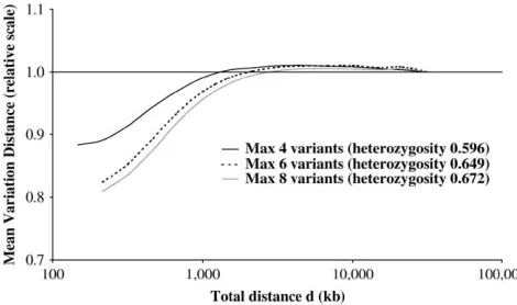
Figure 4 compares the Markov approximation pro-files for the three HaploBlock models with up to four, six, and eight variants per block. Figure 4 shows that, as the number of variants per block is allowed to increase, the improvement in the Markov approximation at short distances becomes more pronounced. In other words, as the allele diversity of the blocks increases, the be-havior of the Markov approximation becomes even less like that for individual SNPs. The values in Figure 4 are
relative to baseline Yd,n measures of 0.310, 0.442, and
0.506 for four, six, and eight variants, respectively. Figure 5 compares the Markov approximation pro-files for the three HaploBlockFinder partitions. Recall that the threshold specifies the percentage of the vari-ation within each block that can be covered by four com-mon variants. Figure 5 shows that, as the threshold is relaxed to allow more variation within each block, there is more improvement in the Markov approximation at short distances. Once again, this shows the effect of al-lele diversity. The values in Figure 5 are relative to
base-line measures of 0.397, 0.550, and 0.631 for coverage thresholds of 70, 80, and 90%, respectively.
Finally, Figure 6 compares the Markov approxima-tion profiles for blocks based on arbitrary groupings of SNPs. Figure 6 shows the effect of increasing the number of SNPs per group on the performance of the Markov approximation. Whereas groups of one or two SNPs perform worse at short distances than at long distances, this relationship is reversed for groups of four SNPs or more. The values in Figure 6 are relative to baselines of 0.051, 0.123, 0.184, and 0.294 for one, two, four, and six SNPs, respectively.
The curves in Figures 4–6 are labeled with the aver-age heterozygosity of their respective inferred markers. Each set of curves shows a clear correlation between increased marker heterozygosity and the increased ac-curacy of the Markov approximation at short distances. As explained later, this relationship stems from the effects of marker heterozygosity on the dynamics of the Markov approximation in a recombining population. Furthermore, Figures 1 and 4–6 all show that the per-formance of the Markov approximation is worse at inter-mediate distances than at both short and long distances. These results are explained in the next section by reference to two contrasting processes of mixing and perturbation.
For all measures, the baseline error measures do not converge to zero at large genomic distances, as would be the case in the absence of linkage disequilibrium. The main reason for this is that our sample size is small—-even if a pair of markers is in perfect linkage equilibrium in a population, a small sample from that population will contain some LD due to sampling error. A second reason is that some long-range LD may be present in the pop-ulation, due, for example, to admixing or preferential mating.
Position profiles: We now assess how the accuracy of the independent and Markov approximations varies along each chromosome in comparison with local
re-combination rates. Statistics Yd,n and Zd,n and average
recombination rates were calculated for a sliding win-dow of 20 Mb across each chromosome. We used fixed
Figure 4.—Comparison of Markov distance profiles for HaploBlock models.
Figure 5.—Comparison of Markov distance profiles for HaploBlockFinder models.
values ofd¼500 kb andn¼4 for all the analyses. Local recombination rates were taken from the deCODE map and aligned against the genome build for our HapMap data, using the University of California Santa Cruz Table
Browser (Konget al.2002; Karolchiket al.2004).
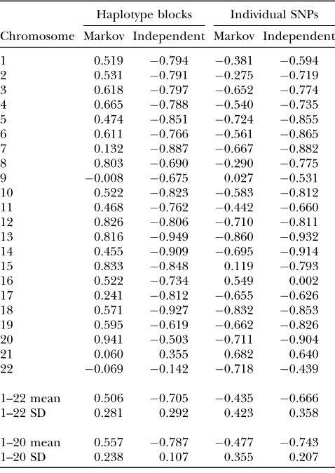
We correlated the error measures and the recombi-nation rates over the window positions for each chro-mosome. Table 3 shows the correlation coefficients for the HaploBlock model with up to four variants per block and for individual SNPs. Windows with low SNP density due to their proximity to a centromere were excluded from these calculations. As can be seen in Table 3, the Markov approximation for the HaploBlock model shows a positive correlation between recombination rates and approximation error, with an average coefficient over
the chromosomes of 0.50660.281. This contrasts with
the independent approximation for the HaploBlock
model, with an average coefficient of0.70560.292.
When considering SNPs individually, a different pic-ture emerges. The error rates of both the independent and Markov approximations are lower in regions of high
recombination, just as in the independent approxima-tion for the HaploBlock model. For the Markov approx-imation over individual SNPs, the average coefficient of
correlation over the chromosomes is 0.435 6 0.423.
The performance of the independent approximation over individual SNPs is similar to that for the
Haplo-Block model, with an average coefficient of0.6666
0.358.
The correlation coefficients for chromosomes 21 and 22 in Table 3 differ significantly from the mean values in many cases. This is because the HapMap data cover just 37 Mb of chromosome 21 and 35 Mb of chromosome 22, so that a sliding window of 20 Mb produces a weak sig-nal. Table 3 also shows the results obtained if these chro-mosomes are removed from the sample, by averaging those for chromosomes 1–20. In all cases, this reduces the standard deviation of the values and strengthens the average correlation.
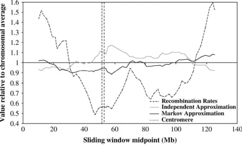
It is instructive to look at one chromosome in more depth, to see an example of how the error measures vary in comparison to local recombination rates. We exam-ine here chromosome 11, since its correlation coeffi-cients as shown in Table 3 are close to the averages over all of the chromosomes. Figure 7 shows how the in-dividual SNP approximation errors vary with recombi-nation rates over the chromosome. As can be seen, the error rates of the two approximations follow each other closely and are strongly anticorrelated with recombi-nation rates. At the ends of the chromosome where recombination rates are highest, both approximations perform well. At the centromere, where recombination rates are generally lower, the opposite effect is seen. In particular, recombination rates near the centromere are
50% of the average, while the Markov and
indepen-dent approximation error is 20–30% higher than the average.
Figure 8 shows the equivalent relationship for the HaploBlock model with up to four variants. The in-dependent approximation performs best at the chro-mosome ends where recombination rates are highest and worst near the centromere where they are low. The TABLE 3
Correlation between recombination rates and error measures for sliding window over individual chromosomes
Haplotype blocks Individual SNPs
Chromosome Markov Independent Markov Independent
1 0.519 0.794 0.381 0.594
2 0.531 0.791 0.275 0.719
3 0.618 0.797 0.652 0.774
4 0.665 0.788 0.540 0.735
5 0.474 0.851 0.724 0.855
6 0.611 0.766 0.561 0.865
7 0.132 0.887 0.667 0.882
8 0.803 0.690 0.290 0.775
9 0.008 0.675 0.027 0.531
10 0.522 0.823 0.583 0.812
11 0.468 0.762 0.442 0.660
12 0.826 0.806 0.710 0.811
13 0.816 0.949 0.860 0.932
14 0.455 0.909 0.695 0.914
15 0.833 0.848 0.119 0.793
16 0.522 0.734 0.549 0.002
17 0.241 0.812 0.655 0.626
18 0.571 0.927 0.832 0.853
19 0.595 0.619 0.662 0.826
20 0.941 0.503 0.711 0.904
21 0.060 0.355 0.682 0.640
22 0.069 0.142 0.718 0.439
1–22 mean 0.506 0.705 0.435 0.666
1–22 SD 0.281 0.292 0.423 0.358
1–20 mean 0.557 0.787 0.477 0.743
1–20 SD 0.238 0.107 0.355 0.207
The haplotype block column refers to the HaploBlock model with up to four variants.
behavior is very similar to that presented in Figure 7 for individual SNPs. By contrast, the Markov approximation for blocks performs worst at the ends of the chro-mosome and best near the centromere. Consequently, unlike the SNP approximations shown in Figure 7, the independent and Markov approximations for haplotype blocks are significantly out of phase.
Figure 9 summarizes the behavior of the Markov posi-tion profiles for all the different models examined. Each point compares the average marker heterozygosity for a particular model against the average gradient for that model of the best-fit line between the Markov error
mea-sure and recombination rates. This gradientDZ/DcM/Mb
measures the strength of the effect of local recombi-nation rates on the local performance of the Markov model. Figure 9 shows that for each set of related mod-els, this strength rises monotonically with the average heterozygosity. In the section that follows, we provide a theoretical explanation for this three-way relationship between heterozygosity, recombination, and the accuracy of the Markov approximation.
ON THE MARKOV MODEL
Mixing and perturbation: We define mixing as the progressive reduction in linkage disequilibrium between the markers on a chromosome, as a result of recombi-nation. In a theoretical closed population with random mating, all markers on a chromosome will converge on
perfect linkage equilibrium (Geiringer 1944).
How-ever, the speed of the mixing process depends on two key factors: (a) mixing is faster between more distant mark-ers due to the higher probability of recombination, and (b) mixing is faster between markers with fewer alleles (e.g., SNPs) since each recombination is more likely to bring the marker distribution closer to equilibrium (Rabaniet al.1998; Ardlieet al.2002; Variloet al.2003). Since the independent approximation error stems from linkage disequilibrium, the speed of mixing also deter-mines the accuracy of this approximation at different distances. An independent model is a special case of a Markov model, so the mixing process also contributes to the accuracy of the Markov approximation.
We introduce here a second process related to recom-bination called perturbation, which affects only the Markov approximation. Perturbation is defined as the introduc-tion of new long-range correlaintroduc-tions between markers on a chromosome, as a result of double recombinations. These long-range correlations contribute to inaccuracy in the Markov model. Let us assume that two parent haplotypes are completely distinct from each other. The joint distribution over any set of markers in the parent haplotypes can be represented perfectly by a Markov model, since the allele at each variable site completely determines that at the next site. However, offspring hap-lotypes produced by double recombination from these parents receive two disjoint sections from one parent, separated by a section from the other parent, as shown in Figure 10. In these cases, the correlation between the disjoint sections cannot be expressed in terms of the intermediate region. Since the Markov model represents only dependencies between immediately adjacent mark-ers, these double recombinations introduce inaccuracy in the Markov approximation for the offspring that was not present in the parents. As with the mixing process, this perturbation effect is strongest where the probabil-ity of recombination is higher, since this also means a higher probability of double recombinations.
Figure 8.—Position profiles for haplotype block models over chromosome 11.
Figure9.—Effect of heterozygosity on average best-fit gra-dient between Markov error and recombination rates.
The perturbation process constitutes a key difference between the dynamics of the independent and Markov models. In an infinite population, the accuracy of the independent approximation for a set of markers in-creases monotonically from one generation to the next. By contrast, the accuracy of the Markov approximation can increase or decrease, depending on the relative in-tensity of the mixing and perturbation processes. As we show later, the perturbation process can be stronger for markers with a larger number of alleles, rendering it more visible for multiallelic haplotype blocks than for biallelic SNP markers. This explains why we see a positive correlation between recombination rates and Markov approximation error for blocks, where perturbation is pronounced, but do not see this effect when modeling individual SNPs where perturbation is weaker.
The complex relationship shown in Figures 1 and 4– 6 between physical distance and the accuracy of the Markov approximation for haplotype blocks is also ex-plained by the balance between mixing and perturba-tion. At short distances, the Markov approximation over blocks is accurate due to the low probability of double recombination and the consequent lack of perturba-tion. At long distances, the Markov approximation over blocks is accurate due to the high probability of recom-bination and the consequent strong mixing. At inter-mediate distances, some perturbation takes place but mixing is weak, so the performance of the Markov ap-proximation over haplotype blocks is at its worst.
Intermixing: For meiotic recombination under ran-dom mating, an offspring haplotype is generated from two parent haplotypes by the process depicted in Figure 10. Two parent haplotypes are selected independently from the source population. The offspring haplotype is generated from these parents by a reading process that crosses over from one parent to the other with
proba-bility uj between markers j and j11, where uj is the
recombination fraction between the markers. As a re-sult, the offspring haplotype can contain alternating stretches of genetic material from the two parents.
Our proof makes use of a different process called intermixing. Figure 11 depicts the intermixing process
with the same crossover points as the meiosis in Figure 10. In intermixing, a large number of parent haplotypes are selected independently from the source population. The offspring haplotype is generated from these
par-ents by a reading process that moves to a newparent
with probability uj between markers j and j11. An
offspring haplotype generated by intermixing with x
crossovers will contain genetic material fromx11
in-dependently selected parents. In contrast to normal meiosis, the theoretical intermixing process cannot in-troduce new long-range dependencies, since the read-ing process never returns to a parent previously used.
The key point for our purposes is that if the first two intermixing parents are the same as those for meiosis, the results of meiosis and intermixing are identical if no more than one crossover took place. With less than two crossovers, intermixing uses only the first two parent haplotypes, producing the same offspring haplotype as meiosis. Differences arise only due to double crossovers, after which meiosis returns to the first parent haplotype whereas intermixing selects a new parent. The proof that follows is based on this similarity between the two processes and the fact that intermixing preserves the Markov properties of a population regardless of how many crossovers take place.
Theorem: Consider a population of infinite size in Hardy–Weinberg equilibrium. This population under-goes random mating and meiotic recombination with-out interference in a series of discrete generations.
Consider a set ofn markers numbered 1,. . .,n, with
recombination fractionujbetween each pair of adjacent
markersjandj11.
Define Pu(x1,. . .,xn) as the haplotype distribution
over sites 1,. . .,nin generationuandQuðx1;. . .;xnÞ ¼ Puðx1ÞQn
1
i¼1 Puðxi11jxiÞ as its Markov approximation.
Similarly,Pu11is the haplotype distribution that emerges
in generationu11 andQu11is its Markov approximation.
We define Zu¼ kPuQuk as the variation distance
between distributions Pu and Qu, and Zu11¼ kPu11
Qu11k. LetDuðjÞ ¼1 P
xjðPuðxjÞÞ
2
be the
heterozygos-ity of sitejin generationu, defined by the probability
that two haplotypes chosen randomly from distribution
Pudiffer at sitej. Our theorem states that forn#5
Zu11#Zu1
1 2
X n1
i¼1
ui
!2
min 1;X
n
j¼3 DuðjÞ
!
: ð1Þ
Thus, the errorZu11of the Markov approximation in
generationu 11 is bounded by the errorZuin
genera-tion u, plus an additional term that depends on two factors. The first factor is the square of the total of the intermarker recombination fractions. The second
fac-tor is the sum of the heterozygosities of sites 3,. . .,n,
bounded to be no more than 1.
A full proof of Equation 1 forn#5 is provided in the
appendix. The outline is as follows. Let P9u11 be the
distribution that emerges from performing intermixing
on generationuandQ9u11be its Markov approximation.
We useP9u11andQ9u11to prove the bound onZu11¼
kPu11Qu11kby applying the triangular inequality
kPu11Qu11k#kPu11Pu911k1kPu911Qu911k1kQu911Qu11k:
The first step is to prove an upper bound onkPu11
P9u11k, the variation distance between the haplotype
dis-tributions generated by meiosis and intermixing. This distance is bounded by12 Pni¼11ui
2
minð1;Pnj¼3DuðjÞÞ. The intuition here is that the results of meiosis and intermixing differ only if there was a double
recom-bination, the probability of which is bounded byPn
1 i¼1 ui
2
. If a double recombination did occur, the probability that the offspring haplotype will differ be-tween meiosis and intermixing is bounded by the sum
of the heterozygositiesDu(j) for sitesj¼3,. . .,n, since
j¼3 is the first site that can be affected by a double
recombination.
The second step is to bound kP9u11 Q9u11k, the
variation distance between the distribution resulting from intermixing and its Markov approximation. We
prove that for n # 5, this distance is no greater than
kPuQuk ¼Zu. This result arises because each crossover
event in intermixing selects a new parent haplotype at random, so no new long-range dependencies are
in-troduced. A proof of this bound forn#5 is provided
in the appendix. We also conjecture that this bound
holds true for all values ofn, as suggested by extensive
simulation.
The final step is to prove thatkQ9u11Qu11k ¼ 0,
namely that the Markov approximations of the dis-tributions arising from meiosis and intermixing are identical. The intuition here is that the Markov approx-imation is entirely determined by the joint distribution over each pair of adjacent sites, and this joint distribu-tion is identical for both intermixing and meiosis.
These results are combined under the triangular in-equality to yield Equation 1:
kPu11Qu11k#kPu11P9u11k1kP9u11Q9u11k1kQ9u11Qu11k
#1
2
Xn1
i¼1
ui
!2
min 1;X
n
j¼3
DuðjÞ
!
1Zu:
The average heterozygosity for individual SNPs in the HapMap data is 0.267. By contrast, all of the HaploBlock and HaploBlockFinder block models have an average heterozygosity of 0.586 or more, more than double that for individual SNPs (see Figure 9). Equation 1 suggests that increased heterozygosity leads to a stronger pertur-bation process, which in turn explains the difference in behavior of the Markov approximation for different types of marker. Nonetheless, since Equation 1 provides only an upper bound, it does not provide a complete explanation of this relationship. More theoretical work is required to identify a lower bound, as well as addi-tional factors that affect the perturbation process.
DISCUSSION
In this work, we assessed the accuracy of the inde-pendent and Markov approximations for representing background variation in the human genome. Using data taken from HapMap, we showed how the approx-imation error varies for different physical distances and along each autosome, when modeling both individual SNPs and haplotype blocks of various models. Our core observation is that the Markov model over haplotype blocks is particularly accurate at representing markers in strong linkage disequilibrium. By reference to the perturbation process, we explained why the Markov ap-proximation exhibits this behavior only when modeling multiallelic haplotype blocks, rather than biallelic in-dividual SNPs.
Our motivation for this work was to assess whether it is important to use a Markov chain to represent haplotype block variation or whether an independent model suf-fices. Clearly, a Markov approximation can represent the variation for a set of markers more accurately than an independent approximation, due to the larger num-ber of parameters available. However, our results show an important additional benefit of the Markov model—that when used with haplotype blocks, it is uniquely suited for modeling genomic variation at high density. Models of background variation combining haplotype blocks and a Markov chain have been used by ourselves and
others (Dalyet al.2001; Andersonand Novembre2003;
Greenspan and Geiger 2004a; Kimmel and Shamir 2004).
The error measure we employed is based on the variation distance between a joint distribution and its maximum-likelihood approximation. We used this mea-sure because it permits direct comparison between the independent and Markov approximations and has an intuitive interpretation in terms of the proportion of a distribution misrepresented by its approximation. How-ever, this measure is not ideal, since it is biased by the
allele frequencies at individual markers, just like thejDj
measure of linkage disequilibrium to which it is related.
It would be fruitful to develop an equivalent of theD9
linkage disequilibrium measure for the Markov model, to overcome this disadvantage. Nonetheless, since our empirical observations were based on averages over large numbers of sites, this shortcoming does not affect the overall patterns observed.
other advantages over arbitrary groups of SNPs in terms of model simplicity and the selection of htSNPs.
We referred above to the dependency of the Markov model on the balance between the mixing and pertur-bation processes. Beyond our initial observations, there is work to be done in understanding how these two pro-cesses interact and in developing more precise criteria for determining when each one plays a more dominant role. It is also desirable to ascertain whether a pop-ulation must contain highly distinct haplotypes for the perturbation effect to be seen. On this point, recent re-search has found an abundance of common haplotypes that differ at almost every site in human populations (Zhanget al.2003). Finally, it would be valuable to gen-eralize our proof to a population of finite size and to
extend it to more thann¼5 sites.
LITERATURE CITED
Anderson, E., and J. Novembre, 2003 Finding haplotype block
boundaries by using the minimum-description-length principle. Am. J. Hum. Genet.73:336–354.
Ardlie, K. G., L. Kruglyakand M. Seielstad, 2002 Patterns of
linkage disequilibrium in the human genome. Nat. Rev. Genet.
3:299–309.
Arnheim, N., P. Calabreseand M. Nordborg, 2003 Hot and cold
spots of recombination in the human genome: the reason we should find them and how this can be achieved. Am. J. Hum. Genet.73:5–16.
Cardon, L., and G. Abecasis, 2003 Using haplotype blocks to map
human complex trait loci. Trends Genet.19:135–140. Daly, M., J. Rioux, S. Schaffner, T. Hudson and E. Lander,
2001 High-resolution haplotype structure in the human ge-nome. Nat. Genet.29:229–232.
Devlin, B., and N. Risch, 1995 A comparison of linkage
disequilib-rium measures for fine-scale mapping. Genomics29:311–322. Gabriel, S. B., S. F. Schaffner, H. Nguyen, J. M. Moore, J. Royet al.,
2002 The structure of haplotype blocks in the human genome. Science296:2225–2229.
Geiringer, H., 1944 On the probability theory of linkage in
Men-delian heredity. Ann. Math. Stat.15:25–37.
Goldstein, D., 2001 Islands of linkage disequilibrium. Nat. Genet.
29:109–111.
Greenspan, G., and D. Geiger, 2004a Model-based inference of
haplotype block variation. J. Comp. Biol.11:493–504.
Greenspan, G., and D. Geiger, 2004b High density linkage
dis-equilibrium mapping using models of haplotype block variation. Bioinformatics20(Suppl. 1): I137–I144.
Hardy, G. H., 1908 Mendelian proportions in a mixed population.
Science18:49–50.
International HapMap Consortium, 2003 The International
HapMap Project. Nature426:789–796.
Jeffreys, A., A. Ritchieand R. Neumann, 2000 High resolution
analysis of haplotype diversity and meiotic crossover in the human TAP2 recombination hotspot. Hum. Mol. Genet.9:725–733.
Jeffreys, A., L. Kauppiand R. Neumann, 2001 Intensely punctate
meiotic recombination in the class II region of the major histo-compatibility complex. Nat. Genet.29:217–222.
Johnson, G. C., L. Esposito, B. J. Barratt, A. N. Smith, J. Heward
et al., 2001 Haplotype tagging for the identification of common disease genes. Nat. Genet.29:233–237.
Karolchik, D., A. S. Hinrichs, T. S. Furey, K. M. Roskin, C. W.
Sugnetet al., 2004 The UCSC Table Browser data retrieval tool.
Nucleic Acids Res.32:D493–D496.
Kimmel, G., and R. Shamir, 2004 Maximum likelihood resolution
of multi-block genotypes. Proceedings of the Eighth Annual International Conference on Computational Molecular Biology (RECOMB 2004), San Diego, March 27–31, pp. 2–9.
Kong, A., D. F. Gudbjartsson, J. Sainz, G. M. Jonsdottir, S. A.
Gudjonssonet al., 2002 A high-resolution recombination map
of the human genome. Nat. Genet.31:241–247.
Liu, J., C. Sabatti, J. Teng, B. Keatsand N. Risch, 2001
Bayes-ian analysis of haplotypes for linkage disequilibrium mapping. Genome Res.11:1716–1724.
McPeek, M., and A. Strahs, 1999 Assessment of linkage
disequilib-rium by the decay of haplotype sharing, with application to fine-scale genetic mapping. Am. J. Hum. Genet.65:858–875.
Morris, A., J. Whittakerand D. Balding, 2000 Bayesian fine-scale
mapping of disease loci, by hidden Markov models. Am. J. Hum. Genet.67:155–169.
Morris, A. P., J. C. Whittakerand D. J. Balding, 2002 Fine-scale
mapping of disease loci via shattered coalescent modeling of ge-nealogies. Am. J. Hum. Genet.70:686–707.
Patil, N., A. J. Berno, D. A. Hinds, W. A. Barrett, J. M. Doshiet al.,
2001 Blocks of limited haplotype diversity revealed by high-resolution scanning of human chromosome 21. Science 294:
1719–1723.
Phillips, M. S., R. Lawrence, R. Sachidanandam, A. P. Morris, D. J.
Baldinget al., 2003 Chromosome-wide distribution of
haplo-type blocks and the role of recombination hot spots. Nat. Genet.
33:382–387.
Rabani, Y., Y. Rabinovichand A. Sinclair, 1998 A computational
view of population genetics. Random Struct. Algorithms12:313– 334.
Sebastiani, P., R. Lazarus, S. T. Weiss, L. M. Kunkel, I. S. Kohane
et al., 2003 Minimal haplotype tagging. Proc. Natl. Acad. Sci. USA100:9900–9905.
Templeton, A., A. Clark, K. Weiss, D. Nickerson, E. Boerwinkle
et al., 2000 Recombinational and mutational hotspots within the human lipoprotein lipase gene. Am. J. Hum. Genet. 66:
69–83.
Tishkoff, S. A., and B. C. Verrelli, 2003 Role of evolutionary
his-tory on haplotype block structure in the human genome: impli-cations for disease mapping. Curr. Opin. Genet. Dev.13:569– 575.
Twells, R. C., C. A. Mein, M. S. Phillips, J. F. Hess, R. Veijolaet al.,
2003 Haplotype structure, LD blocks, and uneven recombina-tion within the LRP5 gene. Genome Res.13:845–855.
Varilo, T., T. Paunio, A. Parker, M. Perola, J. Meyer et al.,
2003 The interval of linkage disequilibrium (LD) detected with microsatellite and SNP markers in chromosomes of Finnish pop-ulations with different histories. Hum. Mol. Genet.12:51–59. Wall, J. D., and J. K. Pritchard, 2003 Assessing the performance
of the haplotype block model of linkage disequilibrium. Am. J. Hum. Genet.73:502–515.
Wang, N., J. Akey, K. Zhang, R. Chakraborty and L. Jin,
2002 Distribution of recombination crossovers and the origin of haplotype blocks: the interplay of population history, recom-bination, and mutation. Am. J. Hum. Genet.71:1227–1234. Zhang, K., and L. Jin, 2003 HaploBlockFinder: haplotype block
analyses. Bioinformatics19:1300–1301.
Zhang, J., W. L. Rowe, A. G. Clark and K. H. Buetow,
2003 Genomewide distribution of high-frequency, completely mismatching SNP haplotype pairs observed to be common across human populations. Am. J. Hum. Genet.73:1073–1081. Zhang, K., P. Calabrese, M. Nordborg and F. Sun, 2002
Hap-lotype block structure and its applications to association studies: power and study designs. Am. J. Hum. Genet.71:1386–1394.
APPENDIX
Here we prove in full the theoretical result outlined in this article.
Definitions: Under meiotic recombination, each offspring haplotype over n sites is formed from two parent
haplotypesy1¼ ðy1
1;. . .;y 1 nÞandy
2¼ ðy2
1;. . .;y 2
whichri¼1 if a crossover took place between sitesiandi11 andri¼0 otherwise. LetF(y1,y2,r) denote the offspring
haplotype that is generated by meiosis fromy1andy2, assuming a crossover vectorr:
Fðy1;y2;rÞ ¼y1Sðr;1Þ;. . .;ySnðr;nÞ: ðA1Þ
In Equation A1,S(r,i) is the index of the parent of siteiin the offspring, namelySðr;iÞ ¼11Pik¼11rkmodulo 2.
If there are an even number of recombinations up to siteithenS(r,i)¼1; otherwiseS(r,i)¼2. Since both parents are
selected randomly from the same distribution, we assumed without loss of generality that the first site in the offspring
comes from parent haplotypey1.
The probability of a crossover occurring between sitesiandi11 is denoted byui. We define the probabilityG(r) of a
crossover vectorrin terms of these pairwise probabilities:
Gðr1;. . .;rn1Þ ¼ Y n1
i¼1
uri
i ð1uiÞ1ri: ðA2Þ
Recall thatPu(x) denotes the frequency of haplotypexin generationu. The frequencyPu11(x) of haplotypexin
generationu11 due to meiotic recombination is the sum of the probabilities of all joint assignments toy1,y2, andr,
which yieldx:
Pu11ðxÞ ¼
X
y1;y2;rjFðy1;y2;rÞ¼x
GðrÞPuðy1ÞPuðy2Þ: ðA3Þ
For intermixing overnsites, each offspring haplotype can inherit sections from up tonhaplotypes in the previous
generation, although in most cases less thannwill be used. LetF9(y1,. . .,yn
,r) denote the haplotype generated from y1,. . .,yn
by intermixing under a crossover vectorr:
F9ðy1;y2;rÞ ¼y1S9ðr;1Þ;. . .;ynS9ðr;nÞ: ðA4Þ
In Equation A4,S9(r,i) is the index of the parent of siteiin the offspring, namelyS9ðr;iÞ ¼11Pik¼11rk. The function
S9(r,i) counts the number of crossovers that have taken place up to sitei. The frequencyP9u11(x) of haplotypexin
generationu11 due to intermixing on parent distributionPuis as follows:
Pu911ðxÞ ¼
X
y1;...;yn;rjF9ðy1;...;yn;rÞ¼x
GðrÞY
n
i¼1
PuðyiÞ: ðA5Þ
Intermixing and meiosis: We prove the following bound on the variation distance between the haplotype
distributionPu11arising from meiosis on generationuand the distributionP9u11arising from intermixing:
kPu11P9u11k#
1 2
Xn1
i¼1
ui
!2
min 1;X
n
j¼3 DuðjÞ
!
: ðA6Þ
Recall thatDu(j) is defined as the heterozygosity of sitejin generationu, whereDuðjÞ ¼1
P
xjðPuðxjÞÞ
2 is the
probability that two haplotypes randomly chosen fromPudiffer at sitej.
LetR¼ f0, 1gn1denote the set of all possible crossover vectorsr. LetRbe the subsetfr 2RjP
jrj#1gconsisting
of crossover vectors representing#1 crossovers, and letR1¼ f
r 2RjPjrj$2gdenote the subset representing$2
crossovers. Clearly,R¼R[R1andR\R1¼Ø. The frequency of haplotypexafter meiosis, given in Equation A3,
can therefore be written as
Pu11ðxÞ ¼
X
y1;y2;r2RjFðy1;y2;rÞ¼x
GðrÞPuðy1ÞPuðy2Þ1
X
y1;y2;r2R1jFðy1;y2;rÞ¼x
GðrÞPuðy1ÞPuðy2Þ: ðA7Þ
Similarly, the frequency ofxafter intermixing, given in Equation A5, can be written as
P9u11ðxÞ ¼
X
y1;...;yn;r2Rj
F9ðy1;...;yn;rÞ¼x
GðrÞY
n
i¼1
PuðyiÞ1
X
y1;...;yn;r2R1jF9ðy1;...;yn;rÞ¼x
GðrÞY
n
i¼1
Recall that ifr2RthenP
jrj#1. In these cases,S(r,i)¼S9(r,i) for alli, yieldingF9(y
1,. . .,yn,r)¼F(y1,y2,r). In other words, when less than two crossovers occur, the haplotype obtained by meiosis is identical to that obtained by
intermixing for the same parentsy1andy2. Consequently, we rewrite Equation A8 as follows:
Pu911ðxÞ ¼
X
y1;y2;r2RjFðy1;y2;rÞ¼x
GðrÞPuðy1ÞPuðy2Þ1
X
y1;...;yn;r2R1jF9ðy1;...;yn;rÞ¼x
GðrÞY
n
i¼1
PuðyiÞ: ðA9Þ
Since the sums in Equations A7 and A9 corresponding to no more than one crossover are identical, the variation
distance betweenPu11andP9u11is due to two or more crossovers:
kPu11P9u11k ¼
1 2 X x X
y1;y2;r2R1jFðy1;y2;rÞ¼x
GðrÞPuðy1ÞPuðy2Þ
X
y1;...;yn;r2R1jF9ðy1;...;yn;rÞ¼x
GðrÞY
n
i¼1 PuðyiÞ
: ðA10Þ
By introducing the unity sumPy3;...;yn
Qn
i¼3PuðyiÞ ¼1 into the first term of Equation A10, we obtain
kPu11P9u11k ¼
1 2 X x X
y1;...;yn;r2R1jFðy1;y2;rÞ¼x
GðrÞY
n
i¼1
PuðyiÞ
X
y1;...;yn;r2R1jF9ðy1;...;yn;rÞ¼x
GðrÞY
n
i¼1 PuðyiÞ
: ðA11Þ
We now derive the bound forkPu11P9u11k, as given by Equation A6. Let [a¼b] denote the function that returns 1
ifa¼band 0 otherwise, and define [a6¼b]¼1[a¼b]. Equation A11 is reformulated as follows:
kPu11P9u11k ¼
1 2 X x X
y1;...;yn;r2R1
GðrÞY
n
i¼1
PuðyiÞ f½Fðy1;y2;rÞ ¼x ½F9ðy1;. . .;yn;rÞ ¼xg # X
r2R1
GðrÞ X
y1;...;yn
Yn
i¼1 PuðyiÞ
1 2
X
x
j½Fðy1;y2;rÞ ¼x ½F9ðy1;. . .;yn;rÞ ¼xj
¼ X
r2R1
GðrÞ X
y1;...;yn
Yn
i¼1
PuðyiÞ ½Fðy1;y2;rÞ 6¼F9ðy1;. . .;yn;rÞ: ðA12Þ
The last equality follows because ifF(y1,y2,r)¼F9(y1,. . .,yn,r) then the expressionj½Fðy1;y2;rÞ ¼x ½F9ðy1; . . .; yn;rÞ ¼xj ¼0 for allx, and ifF(y1,y2,r)6¼F9(y1,. . .,yn,r), thenj½Fðy1;y2;rÞ ¼x ½F9ðy1;. . .;yn;rÞ ¼xj ¼1 for exactly two values ofx, namelyx¼F(y1,y2,r) andx¼F9(y1,. . .,yn,r).
The value [F(y1,y2,r)6¼F9(y1,. . .,yn,r)]¼1 if the haplotype that arises from meiosis is different from that arising
from intermixing. This condition is fulfilled if the haplotypes differ in at least one site. The haplotypes are always identical at sites 1 and 2 since the earliest that an observed double recombination can occur is between sites 2 and 3. In
other words,S(r, 1)¼S9(r, 1) andS(r, 2)¼S9(r, 2) for any crossover vectorr. By summing the possibilities for the
remaining sites 3,. . .,n, we obtain a simple bound:
½Fðy1;y2;rÞ 6¼F9ðy1;. . .;yn;rÞ# X n
j¼3
½yjSðr;jÞ6¼y S9ðr;jÞ
j : ðA13Þ
Equations A12 and A13 yield
kPu11P9u11k#
X
r2R1
GðrÞX
n
j¼3 X
y1;...;yn
Yn
i¼1
PuðyiÞ ½yS ðr;jÞ j 6¼y
S9ðr;jÞ
j : ðA14Þ
Since, in the worst case, every site from the third one onward has a different source under meiosis and intermixing, P
y1;...;yn
Qn
i¼1PuðyiÞ ½y Sðr;jÞ
j 6¼y S9ðr;jÞ
j is the probability that two independently selected haplotypes from distributionPu
differ at sitej. This is precisely the definition of heterozygosityDu(j), so
kPu11P9u11k#
X
r2R1
GðrÞX
n
j¼3
DuðjÞ: ðA15Þ
Since [F(y1,y2,r)6¼F9(y1,. . .,yn
,r)]#1 by definition, an additional bound is obtained forkPu11P9u11k from
Equation A12:
kPu11P9u11k#
X
r2R1
GðrÞ X
y1;...;yn
Yn
i¼1
PuðyiÞ ¼ X
r2R1
Finally, using the probabilityG(r) of a crossover vectorr(Equation A2), we boundPr2R1GðrÞby summing the
probability of every possible pair of crossovers:
X
r2R1
GðrÞ#X n1
i¼1
ui X
n1
k¼i11
uk#1
2 Xn1
i¼1
ui
!2
: ðA17Þ
Equations A15–A17 yield the bound forkPu11P9u11k, given by Equation A6.
Markov accuracy after intermixing: Recall that P9u11(x) is the haplotype distribution that results from
intermix-ing parent haplotype distributionPuand thatQ9u11(x) is the Markov approximation ofP9u11(x). We prove that for
n#5
kP9u11Q9u11k#kPuQuk: ðA18Þ
For haplotypes withn.5 sites, this problem remains open. However, we conjecture that it is true for all values ofn,
as confirmed by extensive simulation studies up ton¼16.
The formula forP9u11(x) in Equation A5 is now rewritten in terms of contiguous sections inherited from a parent,
using the probabilityG(r) of each crossover vectorrand the probability of the parent haplotype sections that lead tox
underr,
P9u11ðxÞ ¼ X
r2R
GðrÞ Y
S9ðr;nÞ
k¼1
Puðxðr;kÞÞ;
where
xðr;kÞ¼xLðr;kÞ;. . .;xUðr;kÞ
Lðr;kÞ ¼minfijS9ðr;iÞ ¼kg
Uðr;kÞ ¼maxfijS9ðr;iÞ ¼kg: ðA19Þ
In Equation A19, the functions L(r, k) and U(r, k) denote, respectively, the first and last sites in the offspring
haplotype that originate from parentS9(r,i)¼kunder crossover vectorr. Recall thatS9(r,i) is the index of the parent
haplotype for siteiof the offspring haplotype when intermixing with crossover vectorr. The termPu(x(r,k)) denotes the
marginal distributionPuðxLðr;kÞ;. . .;xUðr;kÞÞ ¼Px1;...;xLðr;kÞ1;xUðr;kÞ11;...;xlPuðx1;. . .;xlÞ.
The process of intermixing can be viewed as the transformation of a parent haplotype distributionPu into an
offspring distributionP9u11. This transformation can be decomposed into a series of atomic transformations, one over
each possible crossover point. LetP9i
u11 be the haplotype distribution obtained from intermixing if crossovers are
allowed only over sites 1 toi. In other words,P9i
u11is the result of intermixing onPuif all valuesui,. . .,un1are set to
zero. Clearly, the distributionP91
u11equals the parent haplotype distributionPu, sincePu9111is the result of intermixing
if no crossing over is allowed. Similarly, the distribution P9n
u11 equals the distribution P9u11 that emerges from
intermixing over all sites, since the full set of crossovers between sites 1 andnis allowed. As a result, the transformation
Pu/P9u11can be expressed as a series of transformationsPu9111/Pu9211/ /Pu9n11, where each stepP9ui11/P9 i11 u11 in
the series introduces an additional crossover point between sitesiandi11.
LetRibe the set of crossover vectors in which crossovers occur only between sites 1 toi;i.e.,Ri¼ fr2Rjr
i¼0, . . .,rn1¼
0g. LetGi(r) be the probability of crossover vectorr2Ri, defined as follows:
Giðr1;. . .;rn1Þ ¼ Yi1
j¼1
urj
j ð1ujÞ1rj:
Using these definitions, the probabilityP9i
u11ðx) of haplotypexafter intermixing over sites 1,. . . ,iis analogous to
P9u11(x), given in Equation A19:
P9ui11ðx1;. . .;xnÞ ¼ X
r2Ri
GiðrÞ Y
S9ðr;nÞ
k¼1
Puðxðr;kÞÞ ¼ X
r2Ri
GiðrÞ Y
S9ðr;nÞ1
k¼1
Puðxðr;kÞÞ !
The recurrence relation betweenP9i11
u11 andP9ui11is explicated by splittingP9 i11
u11ðxÞinto two parts:
P9ui1111ðxÞ ¼ X
r2Ri11jr
i¼0
Gi11ðrÞ Y
S9ðr;nÞ
k¼1
Puðxðr;kÞÞ1 X
r2Ri11jr
i¼1
Gi11ðrÞ Y
S9ðr;nÞ
k¼1
Puðxðr;kÞÞ
¼ ð1uiÞ X
r2Ri11jr
i¼0
GiðrÞ Y
S9ðr;nÞ
k¼1
Puðxðr;kÞÞ
1ui X
r2Ri11jr
i¼1
GiðrÞ Y
S9ðr;nÞ1
k¼1
Puðxðr;kÞÞ !
PuðxLðr;S9ðr;nÞÞ;. . .;xnÞ:
Ifri¼0 then no recombination took place between sitesiandi11, so the sum overr2Ri11is the same as that overr2
Ri
. Ifri¼1 then the last recombination took place betweeniandi11, soU(r,S9(r,n)1)¼iandL(r,S9(r,n))¼i11.
Consequently,
P9ui1111ðxÞ ¼ ð1uiÞ X
r2Ri
GiðrÞ Y
S9ðr;nÞ
k¼1
Puðxðr;kÞÞ
1ui X r2Ri11jr
i¼1
GiðrÞ Y
S9ðr;nÞ1
k¼1
Puðxðr;kÞÞ !
PuðxLðr;S9ðr;nÞÞ;. . .;xnÞ
¼ ð1uiÞP9ui11ðx1;. . .;xnÞ
1ui X
r2Ri11jr
i¼1
GiðrÞ Y
S9ðr;nÞ2
k¼1
Puðxðr;kÞÞ !
PuðxLðr;S9ðr;nÞ1Þ;. . .;xiÞPuðxi11;. . .;xnÞ: ðA21Þ
We now replace the sum overr2Ri11jr
i¼1 by a different sum overr92Ri, where each vectorr9corresponds to a
vectorrwithout the crossover between sitesiandi11:
P9i11
u11ðxÞ ¼ ð1uiÞPu9i11ðx1;. . .;xnÞ
1ui X r92Ri
Giðr9Þ Y
S9ðr9;nÞ1
k¼1
Puðxðr9;kÞÞ !
PuðxLðr9;S9ðr9;nÞÞ;. . .;xiÞPuðxi11;. . .;xnÞ
¼ ð1uiÞ P9i
u11ðx1;. . .;xnÞ1uiP9ui11ðx1;. . .;xiÞPuðxi11;. . .;xnÞ: ðA22Þ
We have replacedGi
(r) withGi
(r9) in the transformation from Equation A21 to Equation A22 since the functionGi
is
not affected by crossovers after sitei. The functionS9(r,n) in Equation A21 counts the total number of crossovers
represented by vectorr. It is replaced byS9(r9,n)11 in Equation A22 sincer9has one fewer crossover thanr. The
product of marginal distributionsQSk¼9ðr1;nÞ2Puðxðr;kÞÞin Equation A21 is replaced by the productQS
9ðr9;nÞ1
k¼1 Puðxðr9;kÞÞin
Equation A22 since it is related only to chromosomal sections preceding sitei, whose parent haplotypes are identical
underrandr9. Similarly,L(r,S9(r,n)1) in Equation A21 is replaced withL(r9,S9(r9,n)) in Equation A22 since the left edge
of the penultimate contiguous section inrthat ends at siteibecomes the left edge of the last contiguous section inr9.
The distributionP9i
u11is the result of intermixing only up to sitei, so its marginalP9ui11ðxi11;. . .;xnÞover sitesi1 1,. . .,nis the same as the parent marginalPu(xi11,. . .,xn). Consequently, Equation A22 implies that
Pu9i1111ðxÞ ¼ ð1uiÞ Pu9i11ðx1;. . .;xnÞ1uiPu9i11ðx1;. . .;xiÞP9ui11ðxi11;. . .;xnÞ: ðA23Þ
Equation A23 states that the effect of introducing the additional crossover point between sites iandi1 1 is to
reconstitute a proportionuiof the population from the marginal distributions on either side of the crossover point,
leaving the remaining 1uiproportion untouched. Equation A23 also holds in the following marginal form by
summing overx1,. . .,xi1,xi12,. . .,xn:
P9i11
We now show a similar result for the Markov approximationQ9i
u11, defined as follows:
Q9i
u11ðx1;. . .;xnÞ ¼P9ui11ðx1Þ Y n1
j¼1 P9i
u11ðxj11jxjÞ: ðA24Þ
The recurrence relation betweenQ9i11
u11 andQ9ui11is explicated as follows:
Q9i11
u11ðxÞ ¼P9i
11
u11ðx1Þ Y n1
j¼1 P9i11
u11ðxj11jxjÞ
¼P9i
u11ðx1Þ Yi1
j¼1 P9i
u11ðxj11jxjÞ Pu9i1111ðxi11jxiÞ Y n1
j¼i11 P9i
u11ðxj11jxjÞ
¼Q9i
u11ðx1;. . .;xiÞ
P9i11
u11ðxi;xi11Þ P9i11
u11ðxiÞ
Y
n1
j¼i11 P9i
u11ðxj11jxjÞ
¼Q9ui11ðx1;. . .;xiÞ
ð1uiÞP9i
u11ðxi;xi11Þ1uiPu9i11ðxiÞP9ui11ðxi11Þ P9i
u11ðxiÞ
Y
n1
j¼i11
P9ui11ðxj11jxjÞ
¼ ð1uiÞ Qu9i11ðx1;. . .;xiÞ P9ui11ðxi11jxiÞ Y n1
j¼i11
P9ui11ðxj11jxjÞ
1uiQ9ui11ðx1;. . .;xiÞ P9ui11ðxi11Þ Y n1
j¼i11
P9ui11ðxj11jxjÞ
Q9i11
u11ðxÞ ¼ ð1uiÞ Q9ui11ðx1;. . .;xnÞ1uiQ9ui11ðx1;. . .;xiÞ Q9ui11ðxi11;. . .;xnÞ: ðA25Þ
We replaced P9i11
u11ðxiÞ with Pu9i11ðxiÞ at several points above since the intermixing process does not affect the
marginal allele frequencies for any individual site. Similarly, we replacedP9ui1111ðxj11jxjÞwithP9ui11ðxj11jxjÞfor anyj6¼i
since the additional crossover permitted between sitesiandi11 affects only marginal distributions containing bothxi
and xi11. Equation A25 states the analogous result for the series of Markov approximations Qu9111;. . .;Q9
n u11 as
Equation A23 states for the series of distributionsP91
u11;. . .;P9 n u11.
Recall that we aim to provekP9u11Q9u11k#kPuQukforn#5. SinceP9u111 ¼PuandPu9n11¼P9u11, this inequality
can be expressed askP9n
u11Q9 n
u11k#kP9 1 u11Q9
1
u11k. To establish this inequality, we prove that for 1#i#n1,
kP9ui1111Q9ui1111k#kP9ui11Qu9i11k: ðA26Þ
We split the proof of Equation A26 into two cases,i¼1 andi¼2. By considering the haplotypes from their other end
points, these proofs also apply, respectively, fori¼n1 andi¼n2, due to symmetry. This covers all values of 1#i#
n1 providedn#5.
Two properties of variation distance are needed. Given two multivariate distributions A(x, y) and B(x,y) with
marginal distributionsAðxÞ ¼PyAðx;yÞandBðxÞ ¼PyBðx;yÞ, the first property states thatkA(x,y)B(x,y)k $
kA(x)B(x)k. Given two mixture distributionsA(x)¼aA1(x)1(1a)A2(x) andB(x)¼aB1(x)1(1a)B2(x), the
second property states that kA(x)B(x)k # akA1(x)B1(x)k1 (1a)kA2(x)B2(x)k. Proofs of these two
properties are provided at the end of theappendix.
Fori¼1, we prove Equation A26 by rewriting P92
u11 andQ9 2
u11 in terms ofP9
1
u11 andQ9 1
u11, using the recurrence
relations in Equations A23 and A25:
P9u211ðxÞ ¼ ð1u1Þ P9u111ðx1;. . .;xnÞ1u1P9u111ðx1Þ Pu9111ðx2;. . .;xnÞ
Q9u211ðxÞ ¼ ð1u1Þ Q9u111ðx1;. . .;xnÞ1u1Q9u111ðx1Þ Q9u111ðx2;. . .;xnÞ
¼ ð1u1Þ Q91