ISSN: 2252-8938, DOI: 10.11591/ijai.v9.i2.pp244-251 244
Index-based transmission for distributed generation in voltage
stability and loss control incorporating optimization technique
Fareed Danial Ahmad Kahar1, Ismail Musirin2, Muhamad Faliq Mohamad Nazer3, Shahrizal Jelani4,Mohd Helmi Mansor5
1,2Faculty of Electrical Engineering, Universiti Teknologi MARA Malaysia,Shah Alam, Selangor, Malaysia 3,4Faculty of Engineering, Technology and Built Environment, UCSI University, Kuala Lumpur, Malaysia 5Department of Electrical & Electronic Engineering, College of Engineering, Universiti Tenaga Nasional,
Jalan IKRAM-UNITEN, 43000 Kajang, Selangor, Malaysia
Article Info ABSTRACT
Article history: Received Jan 12, 2020 Revised Mar 20, 2020 Accepted Apr 3, 2020
The integration of Distributed Generation (DG) in a distribution network may significantly affect distribution performance. With the penetration of DG, voltage security is no longer an issue in the transmission network. This paper presents a study of Distributed Generation on the IEEE 26-Bus Reliability Test System (RTS) with the use of Fast Voltage Stability Index (FVSI) for determining its location and incorporated with Grasshopper Optimization Algorithm (GOA) to optimize the sizing of the DG. The study emphasizes the power loss of the system in which a comparison between Evolutionary Programming (EP) and Grasshopper Optimization Algorithm is done to determine which optimization technique gives an optimal result for the DG solution. The results show that the proposed algorithm is able to provide a slightly better result compared to EP.
Keywords:
Distributed generation (DG) Evolutionary programming (EP)
Fast voltage stability index (FVSI)
Grasshopper optimization algorithm (GOA)
Optimization technique
This is an open access article under the CC BY-SA license.
Corresponding Author:
Muhamad Faliq Mohamad Nazer, Faculty of Engineering,
Technology and Built Environment, UCSI University, Kuala Lumpur, Malaysia. Email: [email protected]
1. INTRODUCTION
Distributed generation (DG) is a method for improving the qualities of power systems in a distribution area which employs small-scale technologies near to the end users to produce electricity. DG technology offers a number of potential benefits and it often uses a renewable energy to produce electricity. The lower cost and higher power quality and security offered by using DG including fewer natural outcomes than the conventional power generators have resulted more research that are developing the best methods to fully utilize it in the future [1]. DG is expected to be widely used in electric power system planning and market operations, and is showing an important role with the demand for it increasing sharply over the years. Therefore, to meet the rising demand, a more stable and reliable way is needed as economic and environmental concerns have limited the construction of new transmission lines and power plants which may result in voltage instability and power loss [2]. Optimization techniques over the recent years have shown promising results in obtaining an optimal solution for power systems problems. Numerous researchers have been developing new methods to solve various types of problems in power systems and the commonly used method is Genetic Algorithm (GA) which is also similar to Evolutionary Programming (EP) [3-4]. However, although it may show some results, a stand-alone methods may not give a significant result in finding the best solution for overall power system problems Hence, the combination of an index with an optimization
achievable.
2. RESEARCH METHOD
Traditionally the distribution system is designed to operate with a unidirectional power flow and only the transmission is designed for a two-way power flow. It is assumed that electric power always flows from secondary winding of the transformers in the substations to the end feeders when it comes to planning and operation. In [6-8], the authors stated that due to the integration of DG in a distribution network, the network power flow has changed. Ever since the DG method was introduced, the distribution system has become an active system with both energy generation and energy consumption at the load nodes. Therefore, the hierarchical network design and its operation criteria should now be incorporated with bidirectional power flows. The system changes from inactive to an active network with the integration of DG and affects the reliability and operation of the power system network [9-12]. The optimal placement and sizing of DG can improve the voltage stability and decrease power losses while a non-optimal placement and sizing of DG can result in an increase in power losses, and thus affecting its voltage stability by making it higher than the allowable limit. To enable reactive power compensation for voltage control and reducing losses, a correct implementation of DG is needed to give a positive impact in the distribution system.
2.1. Different cases for DG unit implementation
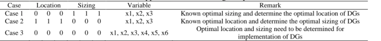
Based on Table 1, different cases of DG problems provide different approaches to solving the problem. In this study, Case 3 is considered where the DG units’ location and sizing are unknown and there are five DG units to be installed in the system. For determining the location of the DG units, an index-based technique will be used for finding the optimal solution to assess the voltage stability of the line so that voltage collapse can be avoided when the DG units are installed. Then, GOA will be implemented to find the optimal sizing of the DG units that has been installed to further enhance their performance by reducing the power losses of the system.
Table 1. Types of cases in solving DG problems
Case Location Sizing Variable Remark
Case 1 0 0 0 1 1 1 x1, x2, x3 Known optimal sizing and determine the optimal location of DGs Case 2 1 1 1 0 0 0 x1, x2, x3 Known optimal location and determine the optimal sizing of DGs Case 3 0 0 0 0 0 0 x1, x2, x3, x4, x5, x6 Optimal location and sizing need to be determined for
implementation of DGs
2.2. Placement of DG units based on FVSI
For the placement of the DG units, since the study focuses on the increment of reactive power load, FVSI is used. Based on the author in [5], FVSI is sensitive towards reactive power load changes. Therefore, FVSI is suitable in this study to calculate the point of voltage collapse of the system in order to determine the location of the DG unit. The fast voltage stability index, FVSI [5] can be defined by:
𝐹𝑉𝑆𝐼 = 4|𝑍|2𝑄2
|𝑉1|2𝑋 (1)
where:
X = line reactance Z = line impedance V1 = sending end voltage
Q2 = reactive power at the receiving end
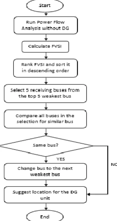
The reactive power load at every load bus is increased and power load flow is used to compute the FVSI of the buses. The maximum loadability for each bus will be sorted in descending order with the smallest value being ranked lowest and conversely. The highest rank implies the weak bus in the system that has the lowest sustainable load. A number of weak buses from the ranking are selected depending on the number of DG units to be installed. The process of the placement of the DG unit is shown in Figure 1.
Figure 1. Flowchart for determining the location of DG units
2.3. GOA for sizing of DG unit
Grasshopper optimization algorithm is a swarm intelligence algorithm that was recently developed by [13-16]. GOA is a population-based technique that mimics swarms' conduct and social interaction with a grasshopper. According to the research in [17-20], GOA managed to outperform several algorithms that iares widely used around the world. The results show a satisfactory rate of exploitation by GOA in solving unimodal test functions and exploring for multi-modal test functions is also intrinsically high. GOA also correctly balances exploration and exploitation when solving composite test functions. In addition, GOA has the ability to outperform several present algorithms in solving present and new optimization issues. Currently, GOA is best suited for single objective problems but the research for developing multi-objective problems has already beguan for better enhancements ion finding the global optimum solution in the future [21-22]. Therefore, this algorithm can contribute into different optimization problems in the real world and it also may be beneficial when tuning the main controlling parameters of GOA. There are three forces that influence the position of each grasshopper. These are the social interaction between the swarm and grasshoppers, gravity forces acting on the swarm, and the wind advection. The mathematical model used for simulating grasshoppers' swarming behavior can be presented as follows [23]:
𝑋𝑖= 𝑆𝑖+ 𝐺𝑖+ 𝐴𝑖 (2)
where Xi is defined as the position of the i-th grasshopper and Si, Gi and Ai represents the social interaction,
gravity force on grasshopper and the wind advection, respectively. From (2), the position of the grasshopper can be derived and defined as follows:
𝑋𝑖= ∑𝑁𝑗=1𝑠(|𝑥𝑗− 𝑥𝑖|) 𝑥𝑗− 𝑥𝑖
𝑑𝑖𝑗 − 𝑔𝑒̂ + 𝑢𝑒𝑔 ̂𝑤 (3)
To solve the optimization problem and prevent the grasshoppers from reaching the comfort zone quickly, and so that the swarm does not converge on the target, from (3) can be modified as follows:
𝑋𝑖= 𝑐 ∑𝑁𝑗=1𝑐( 𝑢𝑏𝑑− 𝐼𝑏𝑑
2 𝑠(|𝑥𝑗 𝑑− 𝑥
𝑖𝑑|) 𝑥𝑗− 𝑥𝑖
𝑑𝑖𝑗 ) + 𝑇̂𝑑 (4)
where ubd is the upper bound in the Dth dimension, lbd is the lower bound in the Dth dimension, 𝑇̂𝑑 is the Dth dimensional value in the target (the best solution found so far), and c is a decreasing coefficient for shrinking
is calculated as follows:
𝑐 = 𝑐𝑚𝑎𝑥 − 𝑙𝑐𝑚𝑎𝑥−𝑐𝑚𝑖𝑛
𝐿 (5)
where cmax and cmin is the maximum and minimum value respectively while l indicates the current iteration and L is the maximum number of iterations. In this work, we use 1 and 0.00004 for cmax and cmin respectively.
The proposed mathematical model requires that grasshoppers gradually move towards the target during iterations. Nevertheless, there is no target in a real search space because the main target, or the global optimum, is unknown. Therefore, in each step of optimization, finding a target for grasshoppers is a must. In GOA, the fittest grasshopper (the one with the best objective value) is assumed to be the target during optimization. This will allow GOA to save in every iteration the most promising goal in the search space, allowing the grasshoppers to push towards it.
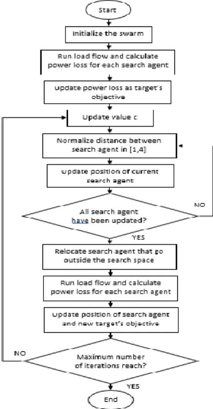
Through creating a set of random solutions, the GOA starts the optimization. Search agents are updating their positions on the basis of (4). In each iteration, the position of the best target achieved so far is updated. Furthermore, the factor c is calculated using (5) and in each iteration the distances between the grasshoppers are normalized in range of [24-25]. The position update is carried out iteratively until an end criterion is satisfied. Finally, the best target position and fitness is returned as the best approach to the global optimum. For the sizing of the DG, the algorithm is used and modified to suit the objective which is to reduce the power loss of the system by determining the size of DG units to be installed in the power system [26]. Therefore, the power loss of the system is updated as the target for all the search agents to reach. As shown in Figure 2, the process starts by initializing the swarm and then calculating the first fitness of each search agent. The power loss is set as the target and factor c is updated using (5) as discussed above. The distance between all search agents is normalized and the position of each search agent is updated. The search agent that went outside of the search is then relocated and the calculation of fitness is done using the updated information. The process continues until the maximum number of iterations has been reached and global optimum is achieved. Therefore, the DG size is based on the position of grasshoppers at the target fitness.
3. RESULTS AND DISCUSSION
This section presents the loss profile for before DGs are inserted and after DGs have been inserted with the sizing done by the GOA algorithm. The test results using GOA will then be compared by using the Evolutionary Programming optimization technique. The line voltage stability index, sizing of DGs and loss profile by using both methods are observed and discussed. The test were all done on the IEEE 26-Bus RTS. 3.1. Behavior of GOA in finding optimal solution
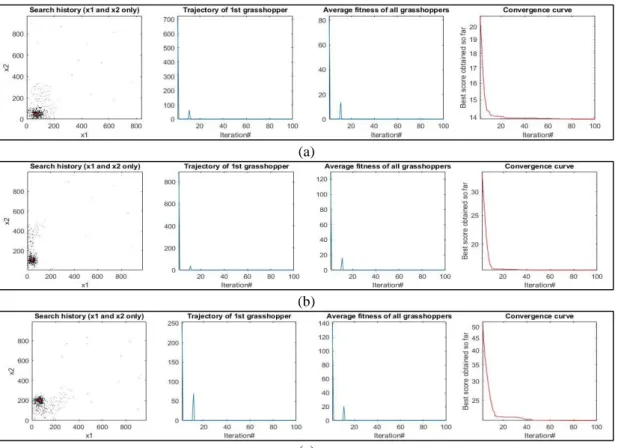
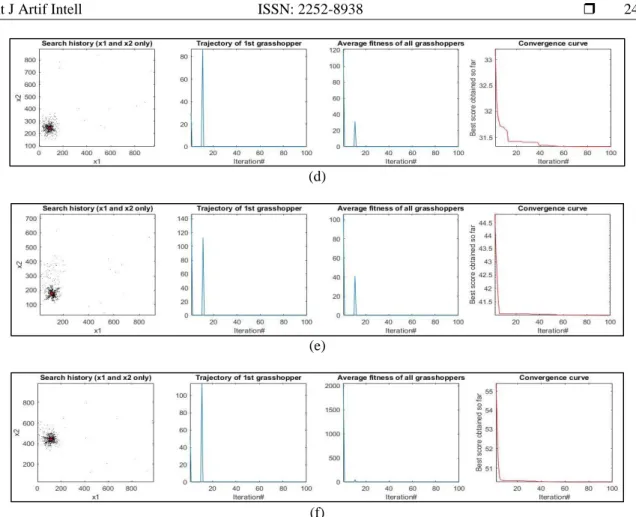
The range of the parameter space is set from 0 to 1000 as shown in the search history in Figure 3. As per the results shown in Figure 3, grasshoppers appear to eventually investigate the promising regions of the search space and cluster around it when the global optima are found. In this IEEE 26-Bus RTS, this trend can be observed. Such results show that exploration and exploitation are beneficially balanced by the GOA algorithm to move the grasshoppers to the optimum region. Furthermore, the attraction between grasshoppers can be observed as all the grasshoppers converge at one point which is the red dot. This is due to GOA's adaptive parameter, which reduces the area of repulsion proportionally to the number of iterations. Therefore, in the final stages of optimization, grasshoppers avoid local valleys in the initial stages of iteration and cluster around the global optimum. The trajectory curves in Figure 3 indicate that in the initial steps of optimization, the grasshoppers show big, abrupt changes. This is because of the high rate of repulsion that causes GOA to explore the search space. It can also be seen that during optimization, the fluctuation gradually decreases due to the adaptive comfort zone and the attraction forces between the grasshoppers. This ensures that the GOA algorithm explores and exploits the search space and eventually converges to a point. Figure 3 shows the average fitness of grasshoppers and convergence curves to support that this action increases the fitness of grasshoppers. The curves clearly show a downward behavior on all reactive load increment. This shows that GOA increases the initial random population and, in the course of iterations, improves the precision of the estimated optimum.
(a)
(b)
(c)
Figure 3. Behavior of GOA on different reactive load increments of (a) 0 MVAR, (b) 18 MVAR, (c) 36 MVAR, (d) 54 MVAR, (e) 72 MVAR and (f) 90 MVAR (continue)
(d)
(e)
(f)
Figure 3. Behavior of GOA on different reactive load increments of (a) 0 MVAR, (b) 18 MVAR, (c) 36 MVAR, (d) 54 MVAR, (e) 72 MVAR and (f) 90 MVAR
3.2. Application of the proposed method 3.2.1. Location suggested using FVSI
Table 2 shows the weakest lines in the power system using the calculated FVSI which indicates that line 1 to line 5 is the top five weakest lines in the power system. Therefore, the location of the DG inserted is at the receiving end of the line since the DG should be located near to the end user to enhance the voltage stability of the system.
Table 2. Five weakest line selected using FVSI
QLOAD (MVAR) Transmission Line
Line 1 Line 2 Line 3 Line 4 Line 5
0 0.0972 0.0939 0.0867 0.0839 0.0829
18 0.1923 0.1771 0.1740 0.1638 0.1466
36 0.3283 0.2761 0.2553 0.2550 0.2427
54 0.4947 0.3819 0.3694 0.3453 0.3405
72 0.6864 0.5341 0.5069 0.4861 0.4535
90 0.9081 0.7978 0.7449 0.6634 0.6277
3.2.2. Loss profile using optimization for DG sizing
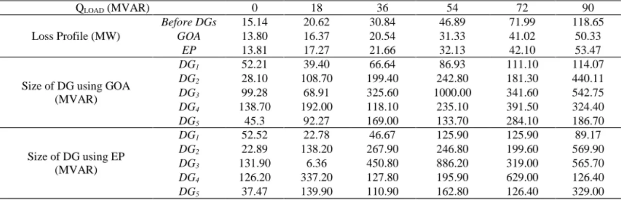
The test is done by adding the reactive power load accordingly to all load buses of the test system. As shown in Figure 4, the power loss curve before inserting DGs is quite high and it increase proportionally when the reactive load is increased. In contrast, when inserting DG by applying the optimization technique for the DG sizing, it shows a significant difference from before the insertion of DGs into the system. However, although the GOA algorithm achieves the lowest total power loss of the system, the gap with the EP optimization technique is not that significant. The GOA and EP curves of the loss profiles are slightly off to each other. In Table 3, the average difference of the loss profile for GOA and EP is just under 2 MW. Therefore, GOA still gives the lowest total loss by estimating the best DG size to be inserted into the power
system. For DG size, the higher the reactive load increase, the higher the overall average size of the DGs. This can also be referred to Figure 4 at the search history of the grasshopper where the higher the increment of the load, the higher the point at which the grasshopper will converge and cluster around. Based on the observation made for the sizing of DG between GOA and EP, the size of the DG for both methods has around 100 to 200 MVAR range of difference on average. Nevertheless, the total loss from the given sizing of both methods are not too far off from one another. Hence, both methods show promising results in finding the right sizing of the DG unit but GOA gives the best global optimum result in total power loss for all load increments.
Table 3. Sizing of DG and the loss profile
Figure 4. Loss profile for before and after inserting DGs using GOA and EP
4. CONCLUSIONS
This paper has presented the index-based transmission for distributed generation in voltage stability and loss control incorporating optimization techniques. It can be concluded that the GOA provides a slightly better result compared to the EP optimisation technique for the IEEE 26-Bus RTS. The proposed index-based technique using FVSI provides adequate information in determining the location of DGs throughout the system in order to maintain its stability of voltage and prevent a collapse. The result shows that this technique is able to perform well for the finding a solution for the optimal location and sizing of DG units.
QLOAD (MVAR) 0 18 36 54 72 90
Loss Profile (MW)
Before DGs 15.14 20.62 30.84 46.89 71.99 118.65
GOA 13.80 16.37 20.54 31.33 41.02 50.33
EP 13.81 17.27 21.66 32.13 42.10 53.47
Size of DG using GOA (MVAR)
DG1 52.21 39.40 66.64 86.93 111.10 114.07
DG2 28.10 108.70 199.40 242.80 181.30 440.11
DG3 99.28 68.91 325.60 1000.00 341.60 542.75
DG4 138.70 192.00 118.10 235.10 391.50 324.40
DG5 45.3 92.27 169.00 133.70 284.10 186.70
Size of DG using EP (MVAR)
DG1 52.52 22.78 46.67 125.90 125.90 89.17
DG2 22.89 138.20 267.90 246.80 199.60 569.90
DG3 131.90 6.36 450.80 886.20 319.00 565.70
DG4 126.20 337.20 127.80 195.90 629.00 126.40
Innovation, and Entrepreneurship (CERVIE).
REFERENCES
[1] Sultana, et al., “An optimization approach for minimizing energy losses of distribution systems based on distributed generation placement,” Jurnal Teknologi, 2017.
[2] Arun Onlam, et al., "Power Loss Minimization and Voltage Stability Improvement in Electrical Distribution System via Network Reconfiguration and Distributed Generation Placement Using Novel Adaptive Shuffled Frogs Leaping Algorithm," Energies, vol. 1, pp. 1-2, January 2019.
[3] Yani, Ahmad, et al., “Optimum reactive power to improve power factor in industry using genetic algorithm,”
Indonesian Journal of Electrical Engineering and Computer Science, pp. 751-757, 2019.
[4] Demir, et al., “Genetic algortihm based resource allocation technique for VLC networks,” pp. 1-4, 2017.
[5] I. Musirin, et al., “Novel fast voltage stability index (FVSI) for voltage stability analysis in power transmission system,” SCORED.2002, pp. 265-268, 2002.
[6] Eslami and Ahmadreza, “Index-Based Optimal DG Allocation for Voltage Quality Improvement in an Unbalanced Network,” 2019.
[7] M. F. Shaari, et al., “Supervised evolutionary programming based technique for multi-DG installation in distribution system,” IAES Int. J. Artif. Intell., vol. 9, no. 1, pp. 11–17, 2020.
[8] S. Vidyasagar, et al., “Optimal Placement of DG Based On Voltage Stability Index and Voltage Deviation Index,”
Indian Journal of Science and Technology, vol 9(38), October 2016.
[9] L. Zhijian, et al., "Optimal power flow research on distributed network considering distributed generation," China
International Conference on Electricity Distribution (CICED), Xi'an, 2016, pp. 1-6, 2016.
[10] C. Ameur, et al., “Intelligent optimization and management system for renewable energy systems using multi-agent,” IAES Int. J. Artif. Intell., vol. 8, no. 4, pp. 352–359, 2019.
[11] K. Lenin, “Dwindling of real power loss by enriched Big Bang-Big Crunch algorithm,” IAES Int. J. Artif. Intell., vol. 7, no. 4, pp. 190–196, 2018.
[12] F. Blaabjerg, et al., “Distributed Power-Generation Systems and Protection,” Proc. IEEE, vol. 105, no. 7, pp. 1311– 1331, 2017.
[13] Z. Wang, et al., “A fully distributed power dispatch method for fast frequency recovery and minimal generation cost in autonomous microgrids,” IEEE Trans. Smart Grid, vol. 7, no. 1, pp. 19–31, Jan. 2016.
[14] S. Wang, et al., “Distributed Generation Hosting Capacity Evaluation for Distribution Systems Considering the Robust Optimal Operation of OLTC and SVC,” IEEE Trans. Sustain. Energy, vol. 7, no. 3, pp. 1111–1123, 2016. [15] G. Chen, et al., “Distributed Optimal Active Power Control of Multiple Generation Systems,” IEEE Trans. Ind.
Electron., vol. 62, no. 11, pp. 7079–7090, 2015.
[16] S. T. Cady, et al., “A Distributed Generation Control Architecture for Islanded AC Microgrids,” IEEE Trans.
Control Syst. Technol., vol. 23, no. 5, pp. 1717–1735, 2015.
[17] S. Ganguly and D. Samajpati, “Distributed generation allocation on radial distribution networks under uncertainties of load and generation using genetic algorithm,” IEEE Trans. Sustain. Energy, vol. 6, no. 3, pp. 688–697, Jul. 2015. [18] T. Wang, et al., “Dynamic Control and Optimization of Distributed Energy Resources in a Microgrid,” IEEE Trans.
Smart Grid, vol. 6, no. 6, pp. 2884–2894, Nov. 2015.
[19] Nguyen, et al., “Distribution network reconfiguration for power loss minimization and voltage profile improvement using cuckoo search algorithm,” Int. J. Electr. Power Energy Syst., pp. 233–242, 2015.
[20] S. A. Shaaya, et al., “Performance comparison of distributed generation installation arrangement in transmission system for loss control,” Bulletin of Electrical Engineering and Informatics, vol. 8, pp. 39-45, 2019.
[21] S. Saremi, et al., “Grasshopper Optimisation Algorithm: Theory and application,” Adv. Eng. Softw., vol. 105, pp. 30–47, 2017.
[22] S. Z. Mirjalili, et al., “Grasshopper optimization algorithm for multi-objective optimization problems,” Appl. Intell., vol. 48, no. 4, pp. 805–820, 2018.
[23] J. Liu, et al., “Coordinated Operation of Multi-Integrated Energy System Based on Linear Weighted Sum and Grasshopper Optimization Algorithm,” IEEE Access, vol. 6, pp. 42186–42195, 2018.
[24] H. Liang, et al., “Modified grasshopper algorithm-based multilevel thresholding for color image segmentation,”
IEEE Access, vol. 7, pp. 11258–11295, 2019.
[25] A. G. Neve, et al., “Application of Grasshopper Optimization Algorithm for Constrained and Unconstrained Test Functions,” Int. J. Swarm Intell. Evol. Comput., vol. 06, no. 03, 2018.
[26] M. F. F. Sahilahudin, et al., “Computational Intelligence Based Technique for Multi-DG Installation in Transmission System,” E3S Web Conf., vol. 152, p. 03001, 2020.