Sharif University of Technology
Scientia IranicaTransactions A: Civil Engineering www.scientiairanica.com
3D estimation of metal elements in sediments of the
Caspian Sea with moving least square and radial basis
function interpolation methods
H.R. Zarif Sanayei
a;, N. Talebbeydokhti
aand H. Moradkhani
b a. Department of Civil and Environmental Engineering, Shiraz University, Shiraz, Iran.b. Department of Civil and Environmental Engineering, Portland State University, Portland, Oregon, USA. Received 23 September 2013; received in revised form 29 October 2014; accepted 3 February 2015
KEYWORDS 3D estimation; Moving least square; Radial basis function; The Caspian sea; Interpolation methods.
Abstract. Spatially continuous data is important in modeling numerical and compu-tational works. Since sampling points are not continuous, interpolation methods should be used to estimate data at unsampled points. In this paper, Radial Basis Function (RBF) and Moving Least Square (MLS) interpolation methods are applied to estimate the concentrations of nickel, mercury, lead, copper, and chromium in the Caspian Sea by programming. Cross validation results are also obtained by RBF and MLS methods and have been compared for Lindane, total DDT, total HCH, total hydrocarbons and total PAH elements. Input data for MLS and RBF are longitudinal, latitude and depth (3D interpolation) at any point. Outputs of MLS and RBF are concentrations of an element at any point. A new method is introduced for dening a constant parameter in RBF. The number of sampling points for calibration and verication tests is analyzed with the values of Root Mean Square Error (RMSE) in pollutant parameters. Optimum selection of MLS parameters is used in this paper. The results of concentration estimation of metal elements in sediments of the Caspian Sea, by MLS and RBF, show that RBF method yields more accurate results than MLS method.
c
2015 Sharif University of Technology. All rights reserved.
1. Introduction
Spatially continuous data (the value of pollution con-centration and sediment concon-centration, the level of water in the groundwater well, the percent value of salinity of water, the weather parameters, the agronomy parameters etc.) are essential in modeling, numerical computations, and management discussions. Environmental managers and scientists require accurate spatially continuous data over the region of
*. Corresponding author. Mobile: +98 917 5370182; E-mail addresses: [email protected] (H.R. Zarif Sanayei); [email protected] (N. Talebbeydokhti); [email protected] (H. Moradkhani)
interest to make eective and condent decisions and justied interpretations [1,2]. Since data sampling in a eld is not spatially continuous, and increasing sampling points are expensive, interpolation methods have been used to estimate an attribute at unsampled points. Many interpolation methods have been created for estimation; each method has its advantages and shortcomings.
A number of researchers investigated sediment load patterns based on discontinuous sampling points by dierent statistical methods [3-6]. Various inter-polation methods were applied to determine pollu-tion patterns in soil [7-13]. Similar researches on spatial rainfall variability by using dierent interpo-lation methods were conducted by Shah et al. [14],
Goovaerts [15], Faures et al. [16] and Chaubey et al. [17].
Jerey et al. [18] interpolated daily climate vari-ables with thin plate smoothing spline method. Daily and monthly rainfalls with ordinary kriging method were estimated based on 4600 locations across Aus-tralia. Lu et al. [19] applied kriging method for sed-iment yield mapping in Yangtze basin, china. Sanders and Chrysikopoulos [20] estimated longitudinal inter-polation of parameters, characterizing channel geom-etry by piece-wise polynomial (linear and cubic) and universal kriging methods. These methods were used for a data set describing cross-sectional properties at 283 stations. The results of the study showed that piece-wise linear interpolation gives close estimation as compared to universal kriging estimates. Therefore, this method was recommended for routine modeling purpose. Lin and Chen [21] proposed a spatial interpolation method by combination of the Radial Basis Function Network (RBFN) and the semivari-ogram (named improved RBFN). They showed that the proposed method can estimate the spatial distribution of rainfall (in china), more precisely, as compared to ordinary kriging and standard RBFN.
Moradkhani et al. [22] explored the applicability of a Self Organizing Radial Basis (SORB) function to one-step ahead forecasting of daily stream ow for Salt River; a sub watershed of the lower Colorado River basin. In their paper, SORB outperformed the two other Articial Neural Network (ANN) algo-rithms, the well known Multi-layer Feedforward Net-work (MFN) and Self-Organizing Linear Output map (SOLO) neural network for simulation of daily stream ow.
Zhou et al. [23] applied a Geographic Information System (GIS)-based chemometric approach to inves-tigate spatial distribution of heavy metals in Hong Kong's marine sediments and their human impacts. Li and Heap [2] showed that four factors in selection of interpolation method are: Nature of the estimation, number of sampling points in km2 or (km2/sample),
region of study, and sampling design in a region. Heritage et al. [24] studied the inuence of survey strategy and interpolation model on Digital Elevation Model (DEM) quality for a gravel bar on the River Nent, Blagill, Cumbria, UK. In their study, digital elevation models were produced using ve dierent common interpolation algorithms.
Merwade [25] evaluated the eect of spatial trend in river bathymetry with isotropic interpolation meth-ods. The results of river bathymetry interpolation will be improved if spatial trends of available data are separated.
An interpolation method which yields good re-sults in a region may not predict accurate rere-sults in another. Therefore, selection of the appropriate
interpolation method in a region is a great challenge. Li and Heap [1] analyzed eciency of 72 spatially interpolation methods/sub-methods in 53 comparative studies (weather sciences, water resource, ecology, agriculture or soil sciences, Limnology etc.). Moreover, sample density and sampling design were evaluated. In their paper, they mentioned that in previous studies: 1) Sometimes the same method was presented with dierent names; 2) Dierent mathematical symbols were often used although they represented the same concept; and 3) Methods were not described clearly in some studies. Li et al. [26] evaluated 14 interpolation methods for distribution of sediments at ve levels of sample density across the southwest Australian margin. Bathymetry, distance to coast, slope and geomorphic province were considered in their interpolation. Ran-dom forest and kriging (Rkrf) methods were realized as best methods for interpolation.
Kazemi and Hosseini [27] estimated heavy metals in sediments consisting of Mercury, copper, Cadmium, Arsenic, Zinc and lead for the Caspian Sea. Ordinary kriging, Genetic Algorithm based on Articial Neural Network (GA-ANN), Adaptive Network Fuzzy Infer-ence System (ANFIS) and Conditional Simulation (CS) were used in their study. Wang et al. [28] used cluster analysis and inverse distance weighted interpolation methods for estimation of water quality, PH, TDS, total nitrogen etc. in three Forks Lake, China.
Kurtulus and Flipo [29] estimated piezometric head with ANFIS model in an aquifer covering 40 km2.
In their study, 73 well data sets were used for watershed in east of Paris in 2009. Cartesian coordinates and elevation of the ground were also considered in their interpolations.
Zhenyao et al. [30] considered the impact of spatial rainfall variability on hydrology and nonpoint source pollution modeling. In their paper, the un-certainty introduced by spatial rainfall variability was determined using a number of commonly used interpo-lation methods; e.g. the centroid method, Thiessen polygon method, Inverse Distance Weighted (IDW) method, the dis-kriging method and co-kriging method. In this study, Radial Basis Function (RBF) and moving least square methods are used for the estima-tion of nickel, mercury, lead, copper, and chromium concentrations in the Caspian Sea. Pollution is a serious and dangerous problem for the Caspian Sea. The conned nature of the sea makes it vulnerable to agricultural, industrial, and oil pollutions.
The results of RBF and MLS cross validation are compared for Lindane, total DDT, total HCH, total hydrocarbons and total PAH. A new method is developed and introduced for 1) Selection of constant parameter in RBF; and 2) The number of stations used for calibration and verication tests. Optimum selection of MLS parameters are used in this paper.
2. Algorithm of Moving Least Square (MLS) interpolation method
This method is one of the best methods for interpola-tion that is briey discussed here (for more details refer to Lancaster and Salkauskas [31]). In this method the point weights are estimated as:
w(i)(z) = j~z ~z ij
=p 1
(x xi)2+ (y yi)2+ (z zi)2
;
(1) where (xi; yi; zi) are coordinates of sampling point, and
(x; y; z) are coordinates of estimation points. As the distance between sampling and estimation points is increased, the eect of sample over the estimated point is decreased. The value of is an even numerical parameter according to Lancaster and Salkauskas [31]. Moreover, is a calibration parameter. After calcula-tion of the weights, w(i)(z) and v(i)(z) are determined
as:
v(i)(z) = Pw(i)(^z) N
j=1w(j)(^z)
i = 1; :::; N; (2)
where N is number of sampling points in the eld. u(i)(^z; z) may now be dened as:
u(i)(^z; z) = b(i) XN j=1
v(j)(^z) b(i)(z
j) i = 1; :::; n;
(3) where ^z is the estimating point, z is the sampling point, b(i) are the values of 1, x, y, x2, xy, y2; ::: for a 2
dimensional eld, and the value of 1, x, y, z, x2, xy,
y2, xz, yz, z2; ::: for a 3 dimensional eld which are
considered in this study. In Eq. (3), n is the number of polynomial terms. In next step sf(^z) is calculated as:
sf(^z) =XN
i=1
fi v(i); (4)
where fi is the value of the case study parameter in
sampling points (value of suspended sediment concen-tration, value of piezometric head in sampling point, etc.). Now, the matrix of (n 1) 1 for a will be calculated as follows:
U(z) W (z) UT(z) = U(z) W (z)
f sf(z) b(1): (5)
Selection of n is related to the number of polynomial terms that are used in this study. For best results in interpolation, cross validation over sampling points could be used. Therefore n is another calibration parameter. U in Eq. (5) is an (n 1) N matrix and
is dened as:
U = 2 6 4
u(2)(^z; z1) u(2)(^z; zN)
... ... ... u(n)(^z; z
1) u(n)(^z; zN)
3 7
5 : (6)
The components of matrix U are obtained from Eq. (3). z1; :::; zN are coordinates values of sampling points and
^z is coordinate of estimated point. In Eq. (5), W (z) is a diagonal matrix of N N that is dened as:
W (^z) = diag (w(^z; z1); :::; w(^z; zN)) : (7)
The components of W (^z) are calculated from Eq. (1). In Eq. (5) the parameter of (f sf(z)b(1)) is a (N 1)
matrix; f is the concentration of the considered element in sampling point; sf(z) is calculated from Eq. (4); and b(1) is the rst element of the polynomial. The
estimation for unsampled points will be calculated by the following equation:
f(^z) = sf(^z) +
n
X
i=1
ai 1(^z) u(i)(^z; z): (8)
All parameters in the above equation are obtained from the previous steps. The steps are repeated for all unsampled points of the eld until a continuous surface is obtained.
3. Algorithm of Radial Basis Function (RBF) interpolation method
Harder and Desmarais [32] and Hardy [33] developed RBF interpolation method. This method is dened as:
^ P (~x0) =
N
X
i=1
Ci ' [k~xi ~x0k] ; (9)
where ~x0 and ~xi are coordinate vectors of estimation
and sampling points, respectively; ^P (~x0) is the value of
estimation attribute in ~x0; N is the number of sampling
points; and Ci's are constant coecients. In Eq. (9),
'[k~xi ~x0k] is one of the RBF functions reported
in Table 1 [34] which depends on relative distance of estimation and sampling points. r2in Table 1 is dened
as: r2= (x
i x0)2+ (yi y0)2+ (zi z0)2; (10)
where zero index is used for estimation points and i
Table 1. RBF functions [34]. '(r) = [r2+ c2]1
2 Multiquadric RBF '(r) = [r2+ c2] 1
2 Inverse multiquadric RBF '(r) = exp[ r2
c2] Gaussion RBF '(r) = [r2+ c2] 1 Couchy RBF
index is used for sampling points. The value of c in RBF functions is a calibration parameter that can be determined from cross validation over sampling points. The process of cross validation will be explained in the next sections. The constant coecients, Ci, in
Eq. (9) are obtained by assuming that ^P (~x0) is one
of the sampling points. Then, Eq. (9) is written for all sampling points and a system of N linear equations and N unknowns is obtained as:
j = 1
P (x1)=' [kx1 x1k]C1+ +' [kxN x1k] CN;
... j = N
P (xN)=' [kx1 xNk]C1+ +' [kxN xNk] CN:
(11)
By solving the above system, Ci's may be found.
The concentration of an element in unsampled point ^
P (~x0) is obtained by substituting the values of Ci and
coordinate vector of unsampled point in Eq. (9).
4. Case study
The case study for interpolation of elements in sed-iments is the Caspian Sea. There are 80 sampling points (stations) for the Caspian Sea in ve countries as shown in Figure 1. The available data for 80 stations were obtained in 2005. There were totally 73 sampling stations: 19 samples from Iran, 18 from Turkmenistan,
16 from Azerbaijan, 12 from Russia, and 8 from Kazakhstan. The sample depths varied from 5 m to 120 m. It should be mentioned that 7 stations located in Volga delta are neglected because no measurement was done in these stations. The concentrations of dierent elements are sampled in these stations. The concentrations of chromium, copper, lead, mercury and nickel will be estimated using RBF and MLS methods. It is worthy to mention here that we do not consider the errors in measurements, because the purpose of this study is to present a new method of data interpolation and not to analyze the measurement biases and errors. However, we know that there exist errors in measurements because of human fault or sampling device imperfections.
The algorithms of MLS and RBF methods are programmed to estimate concentrations of aforemen-tioned elements in the Caspian Sea.
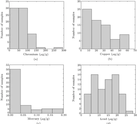
Total hydrocarbons, lindane, total PAH, total HCH, and total DDT are not estimated because of high Root Mean Square Error (RMSE) obtained for sampled points. The data for this study were obtained from www.caspianenvironment.org [35]. The histogram of concentration of chromium, copper, mercury and lead samples are presented in Figure 2.
5. Determination of calibration parameters and cross validation
Calibration parameters in the MLS and RBF methods must be determined before concentrations of elements
Figure 2. The histograms of concentrations of four selected elements: (a) Chromium; (b) copper; (c) mercury; and (d) lead.
are estimated. The calibration parameters are: Num-ber of polynomial terms in MLS(n), power of () in calculation of weights in MLS and the value of c in RBF. Also, the verication test is required to validate interpolation results, and values of n; , and c in RBF and MLS. Therefore, some of sampling points will be considered for calibration of n; and c, and the remaining points are used for verication test.
In cross validation procedure: 1) A value for n; and c will be assumed; 2) One of the sampling points is eliminated; 3) Based on remaining stations and inter-polation method, a value of concentration is estimated for the eliminated point. The estimated concentrations should be compared versus their observed values for all sampling points. The results can be shown on a graph with the observed values in sampling points as horizontal axis and the estimated values as the vertical axis.
RMSE is a measuring tool for determination of discrepancy between the predicted values and the observed ones, and is used to assess the optimum value for n and in MLS and c in RBF. RMSE is described as:
RMSE = sPN
i=2(Poi Pei)2
N ; (12)
where Poi and Pei are values of observation and
estimation in sampling points, N is number of sampling points. The unit of RMSE is microgram over gram (g/g) which is the same as the concentration unit. The values of RMSE, which are close to zero, show perfect interpolation. In order to obtain an RMSE close to zero, the values of n; and c need to be changed. This process is then repeated till the mini-mum RMSE is obtained. The RBF and MLS processes are programmed in this study. Also, calibration and verication test stations are selected randomly. The random selection process should not be in a manner in which complete data for a country in the margins of the Caspian Sea is ignored.
The results of the random selection analysis show that 58 data sets of 73 stations have been used for calibration, and 15 data sets for verication. Figure 3 shows the results of RMSE for 10 parameters in MLS calibration step for = 2 to 10 and n = 4, 10 and 20, respectively. It is observed in Figure 3(a) that, comparing to other values of when = 2, RMSE for all elements, except lindane and nickel, is smaller. In comparison to other values of , RMSE for lindane and nickel are smaller when = 4. It should be noted that the values of RMSE must be compared, in the verication test, for lindane and nickel and then with
Figure 3. Result of RMSE for in calibration step: (a) n = 4; (b) n = 10; and (c) n = 20. 58 data sets are used for MLS calibration.
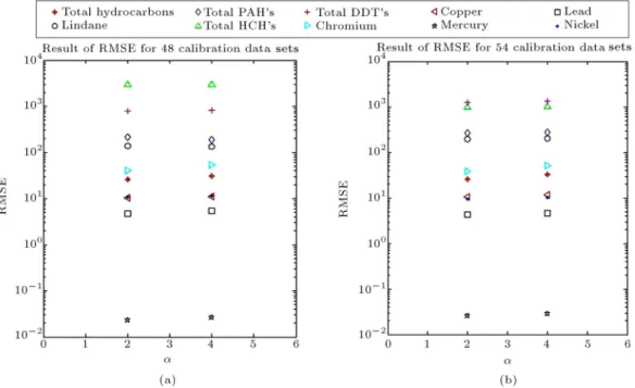
Figure 4. The results of RMSE for 54 and 48 calibration data sets.
regard to dierence of values of RMSE for = 2 and = 4, the value of is selected.
It is noticed that the values of RMSE for n = 10, and n = 20, shown in Figure 3(b) and (c), are more than the values of RMSE for n = 4 (Figure 2(a)). Based on Figure 3, it is observed that the values of RMSE increase in all the elements with increase in n parameter. Thus, the optimum value of n is equal to 4. It is also seen that there are great values of RMSE for lindane, total DDT, total HCH, and total PAH (even greater than 1000). Whereas, chromium, copper, lead, mercury, total hydrocarbon and nickel have suciently small values of RMSE (e.g. smaller than 0.035 for mercury). In this study, the elements with smallest values of RMSE are used for interpolation (chromium, copper, lead, mercury and nickel). In this
study, hydrocarbon is not considered, since its number of samples is low. Figure 4 shows the results of RMSE for 48 and 54 calibration data sets. As shown in Figure 4(a), the values of RMSE in 48 sampling points for lindane, total PAH and total DDT are smaller than those values for 58 sampling points shown in Figure 3(a). However, the three aforementioned elements are not estimated in the present study because of their high values of RMSE. For remaining elements, the values of RMSE for 48 and 54 calibration data sets (shown in Figure 4(a) and (b)) are greater than 58 calibration data sets(shown in Figure 3(a)). As a result, selection of 58 data sets out of 73 total sampling points, for calibration, is optimum.
Up to this point, processes for determination of and n in MLS method have been mentioned. The
process of determination of c in RBF method will be explained hereafter.
In the previous studies, in the literature [1,34], the method of determination of c parameter was not discussed. However, in the present study, the c parameter will be determined such that smallest value of RMSE is obtained using cross validation process.
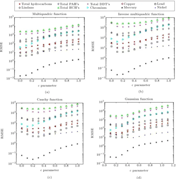
The value of c is dierent for any RBF functions. 58 sampling points are used for calibration of c in the RBF (equal to the number of sampling points in MLS method). For the rst assumption c is considered equal to zero. The value of c will be increased in increments of 0.1 in the code. The process of cross validation is performed in the same way as in MLS method. Then, the value of RMSE will be calculated with dierent c values for each element. Figure 5 shows the value of RMSE for dierent c values and various elements in multiquadric, inverse multiquadric, Cauchy and Gaussion functions. The
RMSE values are increased by increasing c values in all elements for multiquadric function, and the minimum values of RMSE are observed in c = 0 (Figure 5(a)).
Figure 5(b) shows the values of RMSE for inverse multiquadric function. As it is observed, when c = 0:1, the minimum values of RMSE for inverse multiquadric function are greater than the minimum values of RMSE in multiquadric function (Figure 5(a)).
Figure 5(c) shows the values of RMSE for Cauchy function. As it is noticed, the minimum values of RMSE occur in dierent c values (c = 0:1, c = 0:2 and c = 0:3). The minimum values of RMSE for Cauchy function are greater than the minimum of RMSE in multiquadric function (Figure 5(a)).
Figure 5(d) shows the values of RMSE for Gaus-sion function. The minimum values of RMSE for Gaussion function occur in c = 0:1 for chromium, and total hydrocarbons, in c = 0:2 for total HCH, copper,
Figure 5. Results of RMSE for dierent functions in RBF method for dierent values of c: (a) Multiquadric; (b) inverse multiquadric; (c) Cauchy function; and (d) Gaussion function.
lead, and mercury, in c = 0:3 for total DDT, total PAH, and lindane, and in c = 0:5 for nickel.
It is also seen that the minimum values of RMSE for Gaussion function are greater than the minimum of RMSE for multiquadric function (Figure 5(a)).
According to Figure 5(a) to (d), the smallest RMSEs are resulted when multiquadratic function is used. Therefore the multiquadratic function is selected for interpolation of elements in the Caspian Sea.
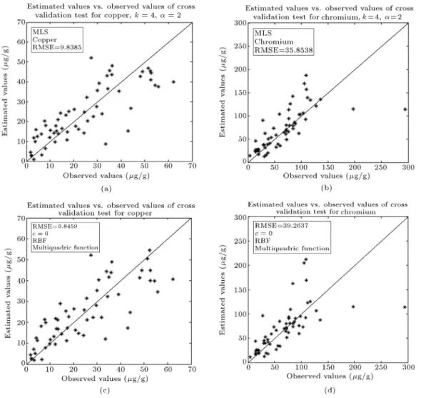
By selecting n = 4 and = 2 in MLS method and multiquadratic function and c = 0 in RBF approach, the cross validation graph can be drawn. Figure 6 shows the results of cross validation for chromium and copper in MLS and multiquadratic RBF interpolation methods. The number of points in Figure 5(a)-(d) is 58 (equal to the number of calibration tests). The bisector line in Figure 6(a)-(d) is in fact the line of perfect estimation. The points above that line represent an overestimation and the below points correspond to underestimation.
Figure 6(a) and (b) show the cross validation graph for copper and chromium, respectively, in MLS.
It is observed that the values of RMSE is equal to 9.83 for copper and 35.85 for chromium (these are the same values in Figure 3(a)).
Figure 6(c) and (d) depict the cross validation graph for copper and chromium, respectively, in RBF. It is noticed that the values of RMSE is equal to 9.84 for copper and 39.26 for chromium (these are the same values of Figure 3).
6. Results of estimation of elements in the Caspian Sea and verication test
After determination of n and in MLS, function used and c in RBF by calibration process and cross valida-tion, concentrations of dierent elements in Caspian Sea are estimated. 169248 unsampled points with known x; y and z coordinates are estimated by MLS and RBF algorithms. Accuracy of interpolation should be determined in MLS and RBF methods with verica-tion test. As it was previously menverica-tioned, 58 data sets of 73 total available data are used for calibration tests, and therefore 15 data sets are remained for verication
Figure 6. Cross validation graphs in calibration step: (a) and (b) Copper and chromium in MLS method, respectively; (c) and (d) copper and chromium in RBF method, respectively.
Figure 7. The results of estimation values for dierent elements in the Caspian Sea.
test. Thus, 15 sampled points are added to 169248 un-sampled points and then these 15 points are estimated the same as other points. Table 2 shows the values of RMSE of verication test for 15 points for dierent elements in MLS and RBF interpolation methods.
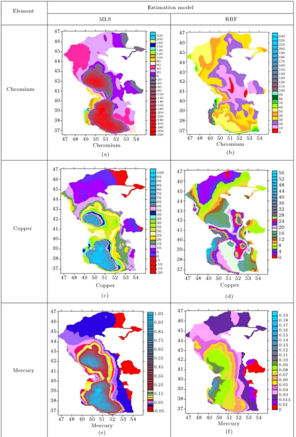
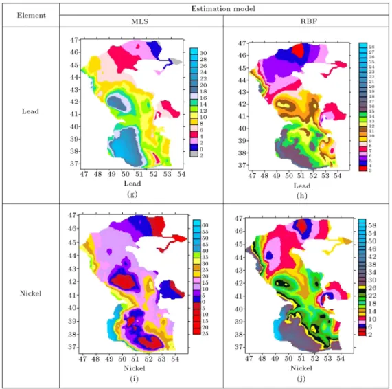
Figure 7 shows the results of interpolation by MLS and RBF methods for ve elements (chromium, copper, lead, mercury and nickel). In this gure, horizontal axis is longitude and vertical axis is latitude and the unit of estimations is microgram over gram (g/g). The
Figure 7. The results of estimation values for dierent elements in the Caspian Sea (continued). Table 2. Results of RMSE in verication test for MLS
and RBF interpolation methods. MLS, n = 4;
= 2
MLS, n = 4;
= 4
RBF, multiquadric,
c = 0 Total hydrocarbons 17.7843 22.1632 22.4403 Lindane 201.8776 195.8664 218.2759 Total PAH's 318.1028 295.1413 314.8002 Total HCH's 800.2946 1615.6104 1547.2669 Total DDT's 949.9851 948.4337 1035.6982 Chromium 23.5205 24.8938 25.3379
Copper 7.7024 9.1648 9.7105
Mercury 0.0174 0.0213 0.0239
Lead 3.2437 3.56 4.0034
Nickel 8.9986 10.40 11.1126
results of estimation patterns in the Caspian Sea can be useful for responsible managers to plan more accurately and comprehensively.
Figure 7(a) and (b) show the estimation of chromium for MLS and RBF, respectively. As
it is observed in Figure 7(a), the estimation of concentration, in MLS method, has negative values in some parts. While, all the RBF estimation values, as shown in Figure 7(b), are positive. It represents the priority of RBF with respect to MLS method. However, the value of RMSE for MLS ( = 2) in verication test (Table 2) is equal to 23.52 which is somewhat smaller than RMSE value of 25.33 in RBF method. This little dierence is negligible compared to the advantage of positive estimation of RBF method. In both gures, the maximum concentration values occur in coasts of Azerbaijan country. The same trend is also observed in Figure 7(c) and (d) for copper, Figure 7(e) and (f) for mercury, Figure 7(g) and (h) for lead, and Figure 7(i) and (j) for nickel concentration. As it is shown in Figure 7(e) and (f), the maximum concentration of mercury takes place in central parts of the Caspian Sea. Figure 7(g) and (f) depict that the maximum concentration of lead occurs in borders of Iran through Azerbaijan. By nding the locations of maximum concentrations of various elements, it will be possible to devise a program with the aim of pollution remedial.
Figure 8. Cross validation graphs in verication step: (a) and (b) Lead in MLS and RBF method, respectively; (c) and (d) nickel in MLS and RBF method, respectively.
Figure 8 shows cross validation graphs in veri-cation test based on 15 points (number of veriveri-cation tests) for lead and nickel. Figure 8(a) and (b) show cross validation graphs in verication test for lead in MLS and RBF methods, respectively. It is observed that the value of RMSE is 3.2437 in MLS (Figure 8(a)) and 4.0034 in RBF (Figure 8(b)). The aforementioned values are the same as those in Table 2. Figure 8(c) and (d) show cross validation graphs in verication test for nickel in MLS and RBF methods, respectively. It is observed that the value of RMSE is 8.9966 in MLS (Figure 8(c)) and 11.1126 in RBF (Figure 8(d)).
7. Conclusion
In this paper, we used a modied version of RBF and MLS interpolation methods to predict the con-centration of heavy metals in the Caspian Sea. It is evident that by increasing the number of samples, the errors associated with interpolation methods reduce. Furthermore, the selection of type of interpolation method is a signicant challenge. It is worthy to mention here that the selection of the best interpolation method is highly case-specic. But, the newly proposed
approach for the selection of and c in MLS and RBF, respectively, can be applied in any other interpolation problems to minimize the RMSE.
According to value of RMSE for cross validation and verication test, interpolation method should be selected. Inputs for this study were longitude, latitude and depth of sampling. The values of RMSE in cross validation for MLS method are smaller than those of RBF. However, the negative values in interpolation are observed for MLS method.
It seems that with conditions discussed and num-ber of available data, RBF method with multiquadric function yields more accurate results (concentration) than MLS method for the Caspian Sea. Basic ideas of this paper are the determination of user constant parameter in RBF and method of cross validation for selection of RBF function. The calculation of the c parameter for RBF is of great importance since previous studies lacked this calculation and only used a guessed value dened by the user. Based on the present study, the maximum concentration values for various elements occur often in coasts of Azerbaijan country, and to some extents in Iran coasts.
Sea can be useful for responsible managers to plan more accurately and comprehensively. By nding the locations of maximum concentrations of various elements, it will be possible to devise a program with the aim of pollution remedial.
References
1. Li, J. and Heap, A.D. \A review of comparative stud-ies of spatial interpolation methods in environmental sciences: Performance and impact factors", Journal of Ecological Informatics, 6, pp. 228-241 (2011).
2. Li, J. and Heap, A. \A review of spatial interpolation methods for environmental scientists", Geosciences Australia, Canberra, No. Record 2008/23 (2008).
3. Phillips, J.M., Webb, B.W., Walling, D.E. and Leeks, G.J.L. \Estimating the suspended sediment loads of rivers in the LOIS study area using infrequent samples", Hydrological Processes, 13, pp. 1035-1050 (1999).
4. Rovira, A. and Batalla, R.J. \Temporal distribution of suspended sediment transport in a Mediterranean basin: The lower Tordera (NE Spain)", Geomorphol-ogy, 79, pp. 58-71 (2006).
5. Nadal-Romero, E., Latron, J., Mart-Bono, C. and Regues, D. \Temporal distribution of suspended sed-iment transport in a humid Mediterranean badland area: The Araguas catchment, central Pyrenees", Geomorphology, 97, pp. 601-616 (2008).
6. Gao, P. and Josefson, M. \Temporal variations of sus-pended sediment transport in Oneida Creek watershed, central New York", Journal of Hydrology, 426-427, pp. 17-27 (2012).
7. Cattle, A.J., McBratney, A.B. and Minasny, B. \Krig-ing methods evaluation for assess\Krig-ing the spatial distri-bution of urban soil lead contamination", Journal of Environmental Quality, 319, pp. 1576-1588 (2002).
8. Atteia, O., Dubois, J.P. and Webster, R. \Geostatisti-cal analysis of soil contamination in the Swiss Jura", Environmental Pollution, 86, pp. 315-327 (1994).
9. Odeh, I.O.A., McBratney, A.B. and Chittleborough, D.J. \Soil pattern recognition with fuzzy c-means: Application to classication and soil-landform interre-lationships", Soil Science Society of America Journal, 56, pp. 505-516 (1992).
10. Franssen, H.J.W.M.H., Van Eijnsbergen, A.C. and Stein, A. \Use of spatial prediction techniques and fuzzy classication for mapping soil pollutants", Geo-derma, 77, pp. 243-262 (1997).
11. Van Meirvenne, M. and Goovaerts, P. \Evaluating the probability of exceeding a site specic soil cadmium contamination threshold", Geoderma, 102, pp. 63-88 (2001).
12. Xie, Y., Chen, T.B., Lei, M., Yang, J., Guo, Q.J., Song, B. and Zhou, X.Y. \Spatial distribution of soil heavy metal pollution estimated by dierent
interpo-lation methods: Accuracy and uncertainty analysis", Journal of Chemosphere, 82, pp. 468-476 (2011).
13. Amini, M., Afyuni, M., Fathianpour, N., Khademi, H. and Fluhler, H. \Continuous soil pollution mapping using fuzzy logic and spatial interpolation", Geoderma, 124, pp. 223-233 (2005).
14. Shah, S.M., O'Connell, P.E. and Hosking, J.R. \Mod-elling the eects of spatial variability in rainfall on catchment response", Journal of Hydrology, 175(1-4), pp. 89-111 (1996).
15. Goovaerts, P. \Geostatistical approaches for incorpo-rating elevation into the spatial interpolation of rain-fall", Journal of Hydrology, 228, pp. 113-129 (2000).
16. Faures, J.M., Goodrich, D.C., Woolhiser, D.A. and Sorooshian, S. \Impact of small scale spatial rainfall variability on runo modeling", Journal of Hydrology, 173, pp. 309-326 (1995).
17. Chaubey, I., Haan, C.T., Grunwald, S. and Salisbury, J.M. \Uncertainty in the model parameters due to spatial variability of rainfall", Journal of Hydrology, 220, pp. 48-61 (1999).
18. Jerey, S.J., Carter, J.O., Moodie, K.B. and Reswick, A.R. \Using spatial interpolation to construct a com-prehensive archive of Australian climate data", En-vironmental Modelling and Software, 16, pp. 309-330 (2001).
19. Lu, X.X, Ashmore, P. and Wang, J. \Sediment yield mapping in a large river basin: The upper Yangtze, China", Environmental Modelling and Software, 18, pp. 339-353 (2003).
20. Sanders, B.F. and Chrysikopoulos, V.C. \Longitudinal interpolation of parameters characterizing channel ge-ometry by piece-wise polynomial and universal kriging methods: Eect on ow modeling", Advances in Water Resources, 27, pp. 1061-1073 (2004).
21. Lin, G.F. and Chen, L.H. \A spatial interpolation method based on radial basis function networks incor-porating a semivariogram model", Journal of Hydrol-ogy, 288, pp. 288-298 (2004).
22. Moradkhani, H., Hsu, K.L., Gupta, H.V. and
Sorooshian, S. \Improved stream ow forecasting using self-organizing radial basis function articial neural networks", Journal of Hydrology, 295, pp. 246-262 (2004).
23. Zhou, F., Guo, H. and Hao, Z. \Spatial distribution of heavy metals in Hong Kong's marine sediments and their human impacts: A GIS-based chemometric approach", Marine Pollution Bulletin, 54, pp. 1372-1384 (2007).
24. Heritage, G.L., Milan, D.J., Large, A.R.G. and Fuller, I.C. \Inuence of survey strategy and interpolation model on DEM quality", Geomorphology, 112, pp. 334-344 (2009).
of river bathymetry", Journal of Hydrology, 371, pp. 169-181 (2009).
26. Li, J., Heap, A.D., Potter, A., Huang, Z. and Daniell, J.J. \Can we improve the spatial predictions of seabed sediments? A case study of spatial interpolation of mud content across the Southwest Australian margin", Continental Shelf Research, 31, pp. 1365-1376 (2011).
27. Kazemi, S.M and Hosseini, S.M. \Camparison of spa-tial interpolation methods for estimating heavy metal in sediment of the Caspian Sea", Journal of Expert Systems with Applications, 38, pp. 1632-1649 (2011).
28. Wang, K., He, P.C., Dong, Y. and Chen, L. \Inverse distance-weighted interpolation to appraising the wa-ter quality of three Froks Lake", Procedia Environmen-tal Sciences, 10, pp. 2511-2517 (2011).
29. Kurtulus, B. and Flipo, N. \Hydraulic head interpo-lation using ANFIS model selection and sensitivity analysis", Journal of Computers and Geosciences, 38, pp. 43-51 (2012).
30. Zhenyao, S., Lei, C., Qian, L., Ruimin, L. and Qian, H. \Impact of spatial rainfall variability on hydrology and nonpoint source pollution modeling", Journal of Hydrology, 472-473, pp. 205-215 (2012).
31. Lancaster, P. and Salkauskas, K. \Surfaces generated by moving least squares methods", Journal of Mathe-matics of Computation, 37(155), pp. 141-158 (1981).
32. Harder, R.L. and Desmarais, R.N. \Interpolation us-ingsurface splines", Journal of Aircraft, 9, pp. 189-191 (1972).
33. Hardy, R.L. \Multiquadric equations of topography and other irregular surfaces", Journal of Geophysical Research, 76, pp. 1905-1915 (1971).
34. Ramachandran, P.A. and Karur, S.R. \Multidimen-sional interpolation using osculatory radial basis
func-tion", Computers and Mathematics with Applications, 35, pp. 63-73 (1997).
35. Www.caspianenvironment.org
Biographies
Hamed Reza Zarif Sanayei is PhD student in Department of Civil and Environmental Engineering at Shiraz University, Iran. He holds BS degree from Shahid Chamran University in Civil Engineering, and MS degree from Shiraz University in Hydraulic Struc-tures.
Nasser Talebbeydokhti is currently Professor of-Civil and Environmental Engineering at shiraz univer-sity. He is Editor in Chief of Iranian Journal of Science and Technology, Transactions of Civil Engineering. Professor Talebbeydokhti is a member of academy of sciences of Iran. He has published many ISI papers. He is actively involved in teaching, research and consulting works in areas of water research, hydraulic structures and environmental engineering.
Hamid Moradkhani holds BS (UT, 1991), MS (IUST, 1994), and PhD (UCI, 2005) degrees, all rst rank, in Civil and Environmental Engineering spe-cializing in hydrology, hydraulics and water resources systems. He has been on the faculty of the Department of Civil and Environmental Engineering at Portland State University (PSU), since September 2006. In 2014, Dr. Moradkhani was elected as a Fellow of American Society of Civil Engineering (F.ASCE). Also, in 2011, he earned the distinction of Diplomate, Water Resources Engineer (D.WRE) recognized and desig-nated by the American Academy of Water Resources Engineers (AAWRE), Board of Trustees.
![Figure 1. Location of sampling points in the Caspian Sea [35].](https://thumb-us.123doks.com/thumbv2/123dok_us/8384894.2227812/4.892.188.692.726.1129/figure-location-sampling-points-caspian-sea.webp)