Sharif University of Technology
Scientia IranicaTransactions C: Chemistry and Chemical Engineering www.scientiairanica.com
Application of conformal mapping to the scattering of
plane SH-waves by a cavity
W. Chen
1;and S.X. Wang
CNPC Key lab of Geophysical Exploration, China University of Petroleum, Beijing, China 102249. Received 23 November 2014; received in revised form 20 August 2015; accepted 24 May 2016
KEYWORDS Conformal mapping; Cavity;
Scattering; Seismic wave; Numerical modelling.
Abstract. In seismic numerical modelling, it is readily to simulate the wave eld of the cavities with simple and regular geometric boundaries. However, the real cavities are always complex or irregular, such as general quadrilateral or horny model. In this paper, conformal mapping is applied to three representative cavity models, including a pentagon model, a generalized quadrangular model, and a horny model. First of all, we transform the original cavity model in the physical domain into a certain simple regular model in the computational domain and, accordingly, transform the boundary condition in the physical domain into that in the computational domain. Then, the wave eld on the boundary in the computational domain is calculated. Finally, we generate the wave eld on the boundary in the physical domain by using the inverse conformal mapping, when the conformal mapping function is invertible. Two experiments by adopting either a displacement boundary condition or a stress boundary condition illustrate that the wave elds for the three dierent kinds of cavities mainly concentrate on the boundary of the corresponding cavity. © 2016 Sharif University of Technology. All rights reserved.
1. Introduction
In exploration geophysics discipline, some cavities in subsurface rocks are often related to reservoirs, since they can load oil or gas. Therefore, it is important to analyze the response character of seismic wave by a ity [1,2]. It is easy to simulate the wave eld of the cav-ities with simple and regular geometric boundaries by using numerical methods or even analytical methods. However, it is dicult to directly simulate a complex or irregular model, which represents real cavity model. The conformal mapping [3] provides an idea which transforms complex or irregular model in the original
1. Present addresses: Key Laboratory of Exploration Technology for Oil and Gas Resources of Ministry of Education, Yangtze University, Wuhan Hubei 430100; and 2Hubei Cooperative Innovation Center of Unconventional Oil and Gas, Wuhan Hubei 430100.
*. Corresponding author.
E-mail addresses: [email protected] (W. Chen); [email protected] (S.X. Wang)
(physical) domain into simple and regular model in the computational domain. In this way, complex or irregular model can be indirectly simulated. In nature, the conformal mapping or some similar techniques, which transform complex or unsolvable or ill-posed problems in the original domain into simple or solvable or well-posed problems in a certain transform domain, have been studied in seismic wave modelling [4,5], seismic processing [6,7], and seismic inversion [8]. In this paper, we apply the conformal mapping to the regular pentagon model, the generalized quadrangular model and the horny model, and analytically derive and numerically simulate the wave eld with either a displacement boundary condition or a stress boundary condition.
2. Theory
2.1. The scattering wave eld
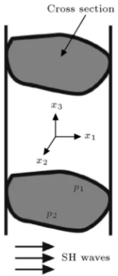
Consider a 3-D isotropic elastic medium embedded into an innitely long cylindrical cavity (Figure 1). The
Figure 1. The cavity model and its boundary p = p1+ p2. The shaded part in the model is the cross
section of the cavity. Cross section is on the x1x2 plane
and the cavity stretches along x3 axis.
elastodynamic equations without body forces can be described as [9]:
lm = uk;klm+ 2"lm; (1)
ml;m= @ 2u
l
@t2 ; (2)
"lm= (ul;m+ um;l)=2; (3)
where lm is the stress, u is the displacement, ()
is Dirac-Delta function, "lm is the strain, and and
are the Lame constants. The subscripts l, m, and k denote three spatial variables. A comma after a quantity denotes partial derivative with respect to spatial variable. For example, ul;m denotes partial
derivative of the displacement along the l direction with respect to spatial variable m.
Substitution of Eq. (1) into Eq. (2) yields the well-known Navier-Cauchy equation:
(clmpqup;q);m= @ 2u
l
@t2 ; (4)
where clmpq is the fourth-order elasticity tensor. The
traditional summation rule over repeated indices is applied throughout this paper.
We consider the scattering problem of plane SH-waves by three kinds of innitely long cylinder cavities with dierent cross sections in this paper. Assuming the cross section is on the x1x2 plane and the cavity
stretches along x3axis (Figure 1), the 3-D problem can
be expressed by a 2-D problem. That means:
u1= u2= 0; (5)
u3= u3(x1; x2; t): (6)
By substituting Eqs. (5) and (6) into Eq. (2), we obtain:
v2
sr2u3=@ 2u
3
@t2 ; (7)
where vs = (=)1=2 is the shear wave velocity, and
r2= @2
@x2 1+
@2
@x2
2 is a Laplace operator.
In the case of steady state, Eq. (7) becomes a Helmholtz equation:
r2u
3+ 2u3= 0; (8)
where = (!=vs)1=2 is the shear wave number.
From Eqs. (1) and (5), we have:
11= 22= 33= 12= 0; (9)
and:
3l= u3;l; (10)
where l is 1 or 2.
For illustrative purposes, complex variable p = x1 + ix2 and its complex conjugate p = x1 ix2 in
the original physical domain (also called p domain) are introduce. In this case, Eqs. (8) and (10) can be rewritten as:
4@p@ p@2u3 + 2u
3= 0; (11)
and: 13=
@u3
@p + @u3
@ p
; (12a)
23= i
@u3
@p + @u3
@ p
: (12b)
Note that the shear modulus lm(l 6= m) is replaced by
symbol lm(l 6= m).
According to Eq. (11), the scattering wave eld w(s) from the cavity meets:
4@@p@ p2w(s)+ 2w(s)= 0: (13)
By substituting a conformal mapping p = F (c) into Eq. (13), we obtain the corresponding equation in the computational domain (also called c domain):
@2w(s)
@c@c = 2
4 dF
dc d F
dcw(s); (14) where c is a point in the computational domain.
After separating the variables c and c, w(s)(c; c)
can be written as: w(s)= w
1(c)w2(c): (15)
integrate operator, we have:
w1(c) = g1()exp [iF (c)=2] ; (16a)
w2(c) = g2()expi F (c)=(2); (16b)
where g1and g2are two constant functions determined
by a separation constant .
Substituting Eq. (16) into Eq. (15) and integrat-ing , the general expression of the scatterintegrat-ing wave eld can be given as:
w(s)=Z
Lg()exp
i2
F (c) +F (c)
d; (17)
where L is a path on the c domain, which is readily chosen to ensure that the integration in Eq. (17) is convergent.
By setting = exp( i1) and F (c) = jF (c)jexp
(i), Eq. (17) can be rewritten as:
w(s)=Z
L iexp( i1)g [exp( i1)] exp
ijF (c)j
cos(1 )
d1=
Z
Lg1[exp( i)]
exp
ijF (c)j cos(1 )
d1: (18)
The function g1[exp( i1)] in Eq. (18) can be spread
into an innite series:
g1[exp( i1)]= 1
X
n= 1
anein1; (19)
where an is the coecients of the series. Introducing a
variable 2= 1 =2, Eq. (18) becomes:
w(s)= X1 n= 1
anexp [in( =2)]
Z
Lexp
in2
ijF (c)j sin 2
d2: (20)
The result of the integration in Eq. (20) is just a Hankel function Hn(1);(2)[jF (c)j].
When jF (c)j ! 1:
H(1);(2)
n [jF (c)j]
s 2 jF (c)jexp
i jF (c)j n 2 4 ; (21)
where Hn(1);(2)() denotes the rst kind and the second
kind of Hankel function for the nth order, respectively.
The scattering wave eld in Eq. (20) should meet the following Sommerfeld radiation condition:
lim
c!1
p
cjw(s)j < M; (22)
lim c!1 p c @w(s)
@c iw(s)
= 0; (23) where M is a nite constant. Thus, we can only choose the rst kind of Hankel function, Hn(1)[jF (c)j].
Consequently, the nal general form of scattering wave eld in the computation domain can be expressed as:
w(s)= X1 n= 1
AnHn(1)(jF (c)j)
F (c) jF (c)j
n
; (24)
where An is an unknown constant, which requires to
be determined from the boundary condition. 2.2. Boundary conditions
In order to calculate the scattering wave eld by Eq. (24), we must rstly get An. The boundary
conditions, such as displacement boundary or stress boundary, need be adopted to solve An.
According to Eq. (12), we have:
13+ i23= 2@w@ p: (25)
To conveniently deal with boundary conditions and boundary value relationship, we bring in curvilinear coordinate system (; ; x3). Assuming that the
inter-section angle of axis and x1 axis is ', the two shear
stress components in the curvilinear coordinate system become:
x3 =13cos ' + 23sin ' =
@w
@pexp(i')
+@w
@ pexp( i')
; (26a)
x3 = 13sin ' + 23cos ' = i
@w
@pexp(i') @w
@ pexp( i')
: (26b)
Consider that the displacement on boundary p1and the
shear stress on boundary p2 are known; the boundary
condition of the steady-state problem can be expressed as:
w = f1(p) 8p 2 p1; (27)
@w
@pexp(i') + @w
@ pexp( i')
= f2(p) 8p 2 p2;
(28) where f1(p) is a known displacement boundary
func-tion, and f2(p) is a known stress boundary function.
Eqs. (27) and (28) are the displacement boundary condition and the stress boundary condition in p do-main, respectively. We will introduce the two boundary conditions in c domain to solve An below.
2.2.1. Displacement boundary condition
According to Eqs. (24), (25), and (27), we obtain:
1
X
n= 1
AnHn(1)(jF j)(F=jF j)n= f1 w(i); (29)
where w(i) is the incident wave eld. In the case of
the polar coordinate c = exp(i), Eq. (30) can be regarded as a function related to angle . To solve An, a term exp( iz)(z = 0; 1; 2; :::) is multiplied
by both sides of Eq. (30). Then, it is integrated from to . Subsequently, Ancan be calculated by solving
the following equation:
1 X n= 1 1 2 Z L()=jL() n H(1) n [jL()] exp( iz)d
An =21
Z
f1()
w(i)()exp( iz)d; (30)
where L() = F (ei).
2.2.2. Stress boundary condition According to the chain rule, we have:
@w @p = 1 F0 @w @c; @w
@ p = 1 F0
@w
@c; (31)
where F0= dF
dc, F0= d dcF.
By substituting Eq. (31) into Eq. (28), we obtain the stress boundary condition in c domain as:
jF0j
c@w
@c + c @w
@c
= f2: (32)
Then, we substitute Eq. (32) into Eq. (24) and obtain:
1
X
n= 1
cF0H
n 1(jc)(F=jF j)n 1cF0Hn+1(jF )
(F=jF j)n+1A n= 2
jF0j
f2 c @w(i)
@c
c@w@c(i)
: (33)
Similar to the steps for deriving Eq. (30) from Eq. (29),
we get the following equation from Eq. (33):
1 X n= 1 1 2 Z cL0H
n 1(jc)(L()=jL()j)n 1
cL0Hn+1(jL())(L()=jL()j)n+1
exp(iz)d
An= 21
Z
2
jL0j
f2
ReL();
ImL()
c@w(i)[ReL(); ImL()] @c
c@w(i)[ReL(); ImL()]@c
exp( iz)d: (34)
2.3. Conformal mapping for three cavity models
In this paper, we design three cavity models, including a regular pentagon model (also called Model 1), a generalized quadrangular model (also called Model 2), and a horny model (also called Model 3). In p domain, it is dicult to calculate scattering wave eld of plane SH-waves by a certain model among the three models. Therefore, we adopt conformal mapping to simplify scattering wave eld modeling, which is performed in c domain.
2.3.1. The conformal mapping for a regular pentagon model
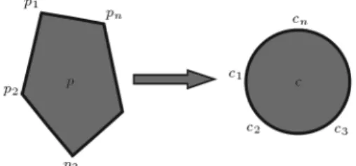
Figure 2 is the conformal mapping from an arbitrary polygon in p domain to a unit circle in c domain. The exterior angles of the arbitrary convex polygon are 1; 2; :::; n and the vertexes of the polygon are
p1; p2; :::; pn. The points c1; c2; :::; cn in c domain
lo-cated on the circumference of the unit circle correspond to p1; p2; :::; pn in p domain, and ck = eik(k =
1; 2; :::; n). On the basis of complex function theory, we have:
p = F0(c) = Gn k=1
1 cckk=; (35) where G is a constant only related to the shape and direction of the polygon. By Eq. (35), an arbitrary
Figure 2. The conformal mapping from an arbitrary polygon to a unit circle.
convex polygon in p domain is transformed into a unit circle in c domain.
According to the binomial theorem, Eq. (35) can be expanded to the following equation:
p = F0(c) = G
1 c1
n
X
k=1
kck+ O(c12)
: (36)
The right side of Eq. (36) is zero if we take the value of variable c on the vertexes. In this way, the character of the conformal mapping p = F0(c) is destroyed on
these vertexes. To overcome this problem, we replace Eq. (36) by a polynomial corresponding with regard to 1=. On the condition of the polygon being equilateral, we denote the exterior angles as k = 2=n(k =
1; 2; :::; n). Furthermore, we assume that the N points, c1; c2; :::; cn, satisfy the equation cn 1 = 0; thus, we
have:
F0(c) = G(1 c n)2
n: (37)
The derivation process of Eq. (37) is described in the Appendix.
For large jcj, Eq. (37) can be expanded as the summation of a power series with regard to 1=c. Thus:
F0(c) = G
1 2
ncn +
2(2 n) 2n2 :
1 c2n + :::
: (38)
Integrating F0(c) and ignoring constant term, Eq. (38)
becomes:
p =F (c) = G
c +n(n 1)2 :cn 11 2n2(2 n)2(2n 1)
: 1 c2n 1+ :::
:
(39) Taking n = 5 and G = 1, and neglecting the high-order terms, we have:
p = F (c) = c +10c14 +75c19: (40) Eq. (40) is a nal expression for the conformal mapping from a regular pentagon to a unit circle (Figure 3).
Figure 3. The conformal mapping from a regular pentagon to a unit circle.
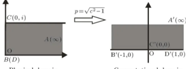
Figure 4. The conformal mapping from a general quadrilateral to an upper half plane.
2.3.2. The conformal mapping for a generalized quadrangular model
Figure 4 is the conformal mapping from a generalized quadrangular model in p domain to an upper half plane in c domain. The cross section of the cavity model in physical domain is marked as ABCD, where point A is located at innite distance, and points B, C, and D are located at nite distance. Note that points B and D are located at the same position. If we calculate the wave eld directly in physical domain, there will be singularity at the vortexes B, C, and D. According to the complex function theory, the problem will be successfully solved if we map the generalized quadrangular in p domain to the upper half plane in c domain. The corresponding conformal mapping is:
p = p0+ K
Z
(c + 1) B=c C=(c 1) D=dc
= p0+ K
p
c2 1; (41)
where K and p0 are two unknown constants. B, C,
and D are the exterior angles on the points B, C,
and D, respectively. According to point B and its corresponding point B', we can get 0 = p0+ A0; thus,
p0 = 0. According to point C and its corresponding
point C', we can get i = Ki, therefore, K = 1. Thus, the conformal mapping is:
p =pc2 1: (42)
2.3.3. The conformal mapping for a horny model Figure 5 is the conformal mapping from a horny model in p domain to an upper half plane in c domain. The are angle of the horny model is =3, the vertex is at the origin point, and angular bisector is along the real
Figure 5. The conformal mapping from a horny model to an upper half plane.
axis. That means:
=6 < argp < =6: (43) For the model, we rst transform the horny model in p domain into right half plane in t domain (or transitional domain) via conformal mapping p = p3t, and then
transform the right half plane to upper half plane in c domain through rotation transform t = ic. In a word, we have the conformal mapping from a horny model to an upper half plane:
p = ip3c: (44)
3. Examples
We consider plane SH-waves propagating on the x1x2
plane in this paper. The incident wave eld is: w(i)= b
0exp [i(p + p)=2] ; (45)
where b0 is the amplitude, which is set as 1.5 in this
paper.
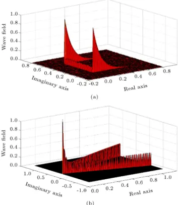
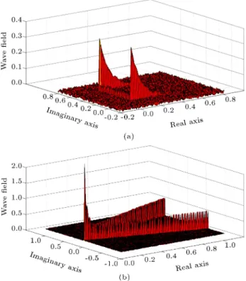
We consider the displacement boundary condi-tion for the rst experiment. As to Model 1, the wave eld on the boundary of the unit circle shows extreme value (Figure 6(a)), which veries the wave eld concentration principle. Note that it is hard to obtain the displacement wave eld in p domain because of the irreversibility of Eq. (41). For Model 2, the variations of the displacement wave eld with position in real axis of Model 2 in c domain are shown in Figure 6(b). There are two peak values corresponding to the two singularities of the model in p domain, namely B(D) and C (Figure 3). By introducing the inverse transformation of Eq. (42) into Eq. (30), we can get the scattering wave eld in the p domain (Figure 7(a)). For Model 3, we select 11 points on the boundary with the distribution of spatial coordinates from -5 to 5 and the interval as 1. By substituting these points into Eq. (31), the displacement wave eld on the boundary is obtained, shown in Figure 6(c). From the gure, we can observe only one extreme point corresponding to the angular point in p domain. In addition, the displacement wave eld on the boundary
Figure 7. The displacement wave eld maps in physical domain for (a) Model 2 and (b) Model 3.
and the angular point focus clearly. By substituting the inverse transformation of Eq. (42) into Eq. (30), we can get the scattering displacement wave eld in p domain (Figure 7(b)).
We consider the stress boundary condition for the second experiment. For Model 1, on the boundary of the unit circle, the stress wave eld in c domain also shows extreme value (Figure 8(a)), similar to the displacement wave eld case (Figure 6(a)). However, curves for the stress wave eld in Figure 8(a) are much rougher than those for the displacement wave eld in Figure 6(a). For Model 2, the variations of the stress wave eld with position in real axis of Model 2 in c domain are shown in Figure 8(b). There are also two peak values corresponding to the two singularities of the model in p domain, namely B (D) and C (Figure 3). By substituting the inverse transformation of Eq. (42)
Figure 6. The displacement wave eld curves with dierent incident angles in the computational domain for (a) Model 1, (b) Model 2, and (c) Model 3.
Figure 8. The stress wave eld curves with dierent incident angles in the computational domain for (a) Model 1, (b) Model 2, and (c) Model 3.
Figure 9. The stress wave eld maps in the physical domain for (a) Model 2, and (b) Model 3.
into Eq. (34), we can get the scattering wave eld in the p domain (Figure 9(a)). For Model 3, we select 21 points on the boundary from -10 to 10 with step 1. By substituting these points into Eq. (34), the stress wave eld on the boundary is obtained, shown in Figure 8(c). From the gure, we can observe only one extreme point corresponding to the angular point in p domain. In addition, the stress wave eld on the boundary and the angular point focus clearly. By substituting the inverse transformation of Eq. (44) into Eq. (34), we can get the scattering stress wave eld in p domain (Figure 9(b)).
The two experiments by using either the dis-placement boundary condition or the stress boundary condition illustrate that the variation trends of the displacement wave eld and those of the stress wave eld are similar. In addition, they both accord with the wave eld concentration principle.
4. Conclusions
By applying conformal mapping to the regular pen-tagon model, the generalized quadrangular model or the horny model, the wave eld in the computational domain is analytically derived and numerically mod-elled with either a displacement boundary condition or a stress boundary condition. When the conformal mapping functions are reversible, the wave elds in the physical domain can also be obtained.
The two experiments illustrate that the wave elds for three dierent kinds of cavities mainly con-centrate on the boundary of the corresponding cavity. It indicates a potential evidence of the existence of cavity, which is probably available information in the oil seismic exploration.
Although the conformal mapping method is ap-plied to the scattering wave eld model for three simplied cavity models with dierent features and shapes in this paper, it can also be used to deal with cavities with arbitrary shapes.
Acknowledgements
This research is partially supported by Sinopec Key Laboratory of Geophysics (Grant No. 33550006-15-FW2099-0017).
References
1. Wang, S.X., Li, X.Y., Qian, Z.P., Di, B.R. and Wei, J.X. \Physical modelling studies of 3-D P-wave seismic for fracture detection", Geophysical Journal of the Royal Astronomical Society, 168(2), pp. 745-756 (2007).
2. Yuan, S.Y., Wang, S.X. and Tian, N. \Min Fres-nel zone relative to large osets", Oil Geophysical Prospecting (in Chinese), 44(4), pp. 387-392 (2009).
3. Gu, X.F. and Wang, Y.L. \Genus zero surface con-formal mapping and its application to brain surface mapping", IEEE Transactions on Medical Imaging, 23(7), pp. 949-958 (2004).
4. Tarrass, I., Giraud, L. and Thore, P. \New curvilinear scheme for elastic wave propagation in presence of
curved topography", Geophysical Prospecting, 59(5), pp. 889-906 (2011).
5. Yuan, S.Y., Wang, S.X., Sun, W.J., Miao, L.N. and Li, Z.H. \Perfectly matched layer on curvilinear grid for the second-order seismic acoustic wave equation", Exploration Geophysics, 45(2), pp. 94-104 (2012).
6. Yu, Y.C., Wang, S.X., Yuan, S.Y. and Qi, P.F. \Phase estimation in bispectral domain based on conformal mapping and applications in seismic wavelet estima-tion", Applied Geophysics, 8(1), pp. 36-47 (2011).
7. Herrmann, F.J., Friedlander, M.P. and Yilmaz, O. \Fighting the curse of dimensionality: compressive sensing in exploration seismology", IEEE Signal Pro-cessing Magazine, 29(3), pp. 88-100 (2012).
8. Yuan, S.Y., Wang, S.X., Luo, C.M. and He, Y.X. \Simultaneous multitrace impedance inversion with transform-domain sparsity promotion", Geophysics, 80(2), pp. R71-R80 (2015).
9. Eduardo, H.M. and Jose P.C. \Asymptotically almost periodic and almost periodic solutions for a class of partial integrodierential equations", Electronic Jour-nal of Dierential Equations, 2006(38), pp. 1-8 (2006).
Appendix
From Eq. (36), we have:
F0(c)=Gn k=1
1 cck
2 n
=cG2n
k=1(c ck)n2: (A.1)
If each c1; c2; :::; cn satises cn 1 = 0, then:
n
k=1(c ck) = cn 1: (A.2)
By substituting Eq. (A.2) into Eq. (A.1), Eq. (37) can be obtained:
F0(c) = G
c2nk=1(c ck)n2
=cG2(cn 1)2 n
= G(1 c n)2
n: (A.3)
Biographies
Wei Chen, a Doctor at China University of Petro-leum-Beijing, was born in December 1985. His research interests include seismic wave eld analysis of hetero-geneous media, seismic physical simulation experiment, and seismic data imaging.
Shangxu Wang, a Professor at China University of Petroleum-Beijing, was born in December 1962. He is currently a Doctoral Supervisor. His research interests include seismic physical simulation experiment, seismic imaging, and seismic data imaging. Professor Wang has made outstanding achievements in the eld of exploration geophysics.