Sharif University of Technology
Scientia IranicaTransactions E: Industrial Engineering www.scientiairanica.com
An ANN-based optimization model for facility layout
problem using simulation technique
P. Azimi
and P. Soo
Faculty of Industrial and Mechanical Engineering, Qazvin Branch, Islamic Azad University, Qazvin, Iran. Received 31 May 2015; received in revised form 12 September 2015; accepted 4 April 2016
KEYWORDS Facility layout; Articial neural network; Discrete-event simulation; Non-dominated sorting genetic algorithm.
Abstract. A real manufacturing system faces lots of real-world situations, such as stochastic behaviors; the lack of attention to this issue is noticeable in the previous research. The aim of this paper is to nd the optimum layout and the most appropriate handling transporters for the problem by a novel solving algorithm. The new model contains two objective functions including the Material Handling Costs (MHC) and the complication time of jobs (makespan). Real-world situations such as stochastic processing times, random breakdowns, and cross tracs among transporters are considered in this paper. Several experiment designs have been produced using DOE technique in simulation software and an Articial Neural Network (ANN) as a meta-model is used to estimate the objective functions in the metaheuristic algorithms. A hybrid non-dominated sorting genetic algorithm (H-NSGA-II) is applied for the optimization task. The proposed methodology is evaluated through a real case study. First, simulation model is validated by comparing it with a real data set. Then, the prediction performance of ANN is investigated. Finally, the ability of H-NSGA-II in searching the solution space is compared with the traditional NSGA-II. The results show that the proposed approach, combing simulation, ANN, and H-NSGA-II, provides promising solutions for practical applications.
© 2017 Sharif University of Technology. All rights reserved.
1. Introduction
A facility layout problem is concerned with determining the arrangement of machines, departments, or cells on the shop oor. The most important performance measure to evaluate the eciency of a layout is the Material Handling Costs (MHC) [1]. Tompkins [2] claimed that 20 to 50 percent of the total operating expenses in manufacturing were attributed to MHC and eective facility layout could reduce these costs by 10 to 30 percent. The ow of materials and the distance between machines are important determinants of MHC. Also, MHC depends on the employed material handling
*. Corresponding author. Tel: 021 22425773; Fax: 021 22425846
E-mail addresses: [email protected] (P. Azimi); parham [email protected] (P. Soo)
vehicles. Material handling vehicles such as forklifts, trucks, and Automated Guided Vehicles (AGVs) are used to transport materials between various points. The type of these transporters inuences the layout of the machines and vice versa. In traditional systems, the decisions related to material handling systems are made after nalizing the layout or vice versa. According to Meller and Gau [3], there exists a lack of parallel engineering in selecting the material handling system with respect to the facility layout. The lack of concurrent engineering results in a high degree of disharmony between the facility layout and material handling system. Therefore, the decisions on deter-mining the type of material handling equipment and the place of machines should be made simultaneously.
While MHC remains the critical index of layout eciency, shorter cycle times have become much im-portant in today's manufacturing systems [4]. Today's
consumer market demands that manufacturers must be competitive. This requires ecient operation of man-ufacturing plants and their ability to satisfy customer demand as quick as possible. On-time delivery and short manufacturing cycle times, as practical issues, should be considered during the layout design process. This paper considers both MHC and completion time of jobs (makespan) as optimality criteria of the layout. To be more practical, this paper takes the stochastic nature of transporters handling time and transporters failure into account when calculating the makespan. Also, this paper considers eect of workow interference as a major concern, which has previously been considered very poorly, in estimating the makespan. The cross trac of transporters can result in considerable delays [5]. These delays lead to an increase in cycle times of production system. Consequently, by taking into account the above factors, we estimate the makespan with the highest possible precision. Because of the described complexity of the manufacturing system, a closed-form analytical expres-sion to calculate makespan does not exist. Therefore, we utilize an Articial Neural Network (ANN) to estimate the makespan. More specically, we rst build a series of random layout designs and then discrete-event simulation model is used to evaluate the makespan of these designs. The obtained makespan is applied to structure an ANN. The ANN works as makespan estimator during the search process. In order to search the solution space, a hybrid algorithm based on non-dominated sorting genetic algorithm (NSGA-II) and an adaptive local search are devel-oped. The remainder of this paper is organized as follows.
Section 2 reviews the existing literature. Section 3 presents the mathematical formulation and properties of the problem. Section 4 explains the proposed methodology. To show performance of the suggested method, computational experiments are done in Sec-tion 5. Finally, the possible extensions of this research are listed along with the conclusions on the proposed approach.
2. Literature review
There is no research similar to the work accomplished in this paper as we review a series of approximately correlated studies. Rosenblatt [6] was the rst who introduced the concept of multi-objective approach to facility layout problems. He considered both qualita-tive and quantitaqualita-tive objecqualita-tives together to come up with a multi-objective formulation. Rosenblatt also proposed a graphical method to generate a series of ecient solutions based on the conicting objectives of minimizing the ow cost and maximizing the closeness rating.
Simulation is known as a powerful tool to evaluate various alternatives of facility layout. Computer simu-lation has been applied in dierent facility layout prob-lems (for example, see [4,7-11]). Gupta [12] employed a simulation model to select the best layout from a set of candidate layouts. He rstly generated a number of material ows based on a predened probability distribution and found the optimum layouts of each ow. He dened the best solution as the layout with each department pair being separated by the average distance of the generated layouts. Then, the exibility of the layout was measured by evaluating its deviation from the ideal distances.
According to Grajo [13], layout optimization and simulation are two tasks that are crucial to any facility planning and layout study. This is because simulation models can reect all of the attributes of real systems that are dicult to consider using analytical models for the layout optimization problems. Azadivar and Tomp-kins [14] suggested a simulation model with a GA-based optimization algorithm. In their method, simulation models were used to evaluate the objective functions and GA-based algorithm was used to search the op-timum solution. Azadivar and Wang [4] presented a facility layout optimization technique that considered the dynamic features and operational constraints of the system as a whole. In their proposed approach, the performance measures of system, such as cycle time and productivity, were evaluated by simulation. Pagell and Melnyk [9] investigated three layouts consisting of the existing worker-paced assembly line, a modied assembly line, and service cells to improve the overall operation of a service process. They used computer simulation to stimulate a critical analysis of the pro-cess.
Kulturel-Konak et al. [15] presented a case in which the demand rate was considered as a stochastic parameter. They also allowed routing exibility for the products so that they were permitted to follow dierent routes in the facility. They used a simulation approach to model the uncertainty. In their simulation, the mean, variance, and covariance of interdepartmental ows were estimated; then, these estimations were used in the design process. Tabu search metaheuristic was employed to solve the problem. Jithavech and Krishnan [11] presented a simulation-based method to evaluate the uncertainty associated with the layout. They validated their simulation model against analyt-ical methods. Results from case studies showed that the simulation-based procedure resulted in reduction of risk as high as 80%. Zhou et al. [10] introduced a method where simulation was combined with Ge-netic Algorithm (GA) to optimize the layout. They tested the optimized site layout within a simulation environment. Altuntas and Selim [16] proposed four dierent weighted association rule-based data mining
approaches to solve facility layout problem. They constructed a simulation model and compared the layouts obtained by the proposed approaches in terms of ve performance measures, namely machine utiliza-tion, total amount of products produced, cycle time, transfer time, and waiting time in queue. Dombrowskia and Ernst [17] presented a scenario-based simulation approach that used scenario technique, morphological analysis, and discrete event simulation to nd out factory layout. Karpe et al. [18] presented a state of the art review of simulation methods for facility layout problems. Azadeh et al. [19] presented an integrated computer simulation-stochastic data envel-opment analysis approach to deal with the facility layout problem. In their research, computer simulation network was used for performance modeling of each layout design. The outputs of simulation were average time-in-system, average queue length, and average machine utilization. By comparing their study with some of the relevant studies and methodologies in the literature, they revealed the high ability of the method to handle complex layout problems in manufacturing systems.
This is the rst study that introduces an inte-grated computer simulation, ANN, and H-NSGA-II as an optimization approach for handling imprecision and non-linearity of layout problems in a special case of manufacturing system.
3. Problem description
The manufacturing system addressed here consists of m machines in which n types of parts, each requiring a set of operations, are to be processed. During the manufacturing process, the transporters move the materials from one machine to another until all the processes are completed. The transporters' handling time is stochastic with known probability distribution. A desired design for the system requires an ar-rangement of m machines in m predened positions and assignment of transporters to each pair of machines such that both MHC and makespan are minimized. Since minimization of MHC does not match minimiza-tion of makespan, the problem falls into the class of multi-objective optimization problems. To explain the conict between two objective functions, adapted from Chiang et al. [20], an eight-machine example with the workow matrix has been shown in Figure 1. The solution to this problem using MHC-based layout is shown in Figure 1(a). While this layout planning will minimize the MHC, it is clear that there are numerous points at which transporters interference occurs. An alternative layout, taking workow interference into account, can be providing a workow in which there are any conicting workows (Figure 1(b)).
Other assumptions considered are as follows:
The distances between machines are determined a priori;
Flow between machines is deterministic;
Machines and locations are of equal size;
The initial allocation cost of a machine in a location is ignored;
The transporters' failure may occur, which leads to increase in their processing time.
3.1. Model formulation
In this section, the nonlinear integer programming formulations of the problem are presented. Before proceeding to the mathematical model, we introduce the indices, parameters, and decision variables: Indices and parameters
i; j Index of machines k; l Index of locations tr Index of transporter
M The number of machines or the locations
Fi;j Amount of material ow among
machines i and j
Dk;l The distance between the locations k
and l
Ci;j Unit material handling cost between
machines i and j
Figure 1. Solution to the eight-facility example: (a) Minimizing MHC, and (b) minimizing workow interference [20].
F Ctr Fixed cost of establishing the
transporter type tr
mtr Maximum available transporter type tr
captr Capacity of the transporter type tr
Decision variables Xi;k 8 > < > :
1; if the machine i
is assigned to the location k 0; otherwise Ytr i;j 8 > < > :
1; if the transporter tr is selected to transfer parts from the machine i to the machine j 0; otherwise
MinZ1=
XM i=1 M X j=1 M X k=1 M X l=1 T R X tr=1 Fi;j captr Ci;j
Dk;l Xi;k Xj;l Yi;jtr
+XM
i=1 M X j=1 T R X tr=1 Ytr
i;j F Ctr; (1)
MinZ2= Makespan; (2) M
X
k=1
Xi;k= 1; 8i = 1; 2; :::; M; (3)
M
X
i=1
Xi;k = 1; 8k = 1; 2; :::; M; (4)
T R
X
tr=1
Ytr
i;j= sgni;j; 8i = 1; 2; :::; M 1;
8k = i + 1; 2; :::; M; (5)
sgni;j 8 > < > :
1; if Fi;j> 0
8i; j = 1; 2; :::; M 0; otherwise (6) Ytr
j;i= Yi;jtr; 8i; j = 1; 2; :::; M; 8tr = 1; 2; :::; T R;
(7)
M 1X i=1
M
X
j=i+1
Ytr
i;j mtr; 8tr = 1; 2; :::; T R; (8)
Xi;k; Yi;jtr2 f0; 1g; i; j; k = 1; 2; ::; M;
8tr = 1; 2; :::; T R: (9) The rst term of objective function (1) is related to
the variable MHC and the second term of it is related to xed cost of the transporters. The rst objective function of the problem is computed by analytical relationships and it focuses on minimizing the handling costs. Objective function (2), which is evaluated by ANNs, focuses on minimizing the whole processing completion time. Constraint set (3) states that each machine is assigned to a location and Constraint set (4) guarantees that each location is occupied by only one machine. Constraint set (5) allocates a trans-porter for movement between two special machines only when material ow exists. Constraint set (8) controls the maximum available number of each type of transporters. The decision variables are kept either at 1 or at 0 by Constraint set (9).
4. Proposed ANN-based optimization
Because of complexity and uncertainty of many real-life problems, it is very dicult to create a precise analytical model. In such complicated situations, simulation is proven as a powerful computer-based tool that can be used instead of the analytical models to study the behavior of complex real systems [21]. Even though simulation models are skillful in capturing complex system behaviors, simulation is essentially a test approach and the way to get the optimum solutions is not clear in it. Therefore, as Fu [21] pointed out, there is a need to develop algorithms that take advantage of the optimization technique, while being as accurate as simulation. The principle of simulation optimization is that during the optimization process, objective function and constraints are evaluated by simulation model.
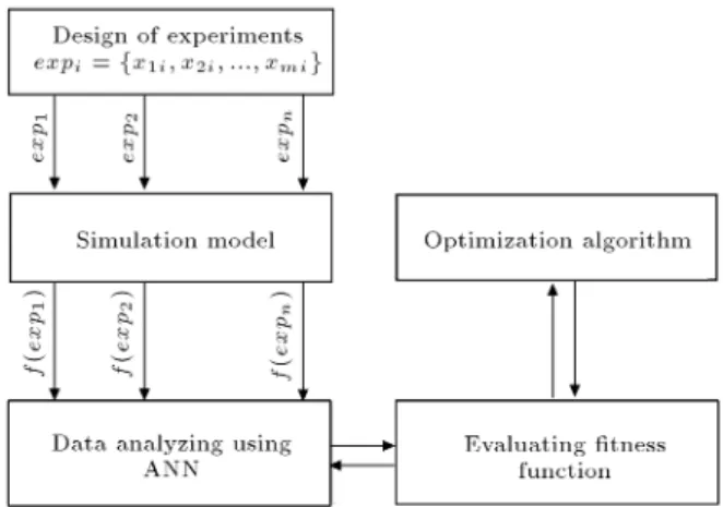
Another weakness of simulation model comes from its requirement of a number of replications, which usually make simulation a very time consuming pro-cess. In order to take a step towards lling this gap, this paper proposes a novel simulation-based optimization framework, which integrates the simulation modeling, articial neural network, and metaheuristic optimiza-tion algorithm. The framework is shown in Figure 2. A series of dierent scenarios are generated. Then, based on these scenarios, discrete event simulation model is run. This input-output data is used to train an ANN to approximate the objective function. ANN acts just like a tremendous intelligent brain, which is trained by simulation data and has the capability to estimate the makespan as fast as analytical relationships and as accurate as simulation models.
To search the solution space, a multi-objective optimization algorithm, called NSGA-II, has been com-bined with an adaptive local search. The NSGA-II showed the capacity to robustly solve large complicated multi-objective problems [22]. In our hybrid NSGA-II (H-NSGA-NSGA-II), ANN is considered as a chromosomes
Figure 2. Framework of the proposed method.
tness function evaluator. The combination of sim-ulation, ANN, and optimization technique provides an eective means for the high complex optimiza-tion problems. For more informaoptimiza-tion on simulaoptimiza-tion- simulation-optimization approaches, advances, and applications, we refer readers to recent reviews by Swisher et al. [23] and Fu et al. [24].
4.1. Articial neural networks
Articial Neural Networks (ANNs) are known as ef-fective techniques for approximating non-linear model functions [25]. Considering the highly non-linear re-lation between the makespan and the selected trans-porters, the ANNs can be eectively applied to nd this indenite relation. ANNs consist of dierent interconnected processing elements that aim to solve a specic problem. These small computing elements are called neurons (Figure 3). The neuron takes inputs, processes them, and transfers the outputs. Neurons are connected to each other by links known as synapses, and associated with each synapse there is a weight factor. First, all the input signals, design conguration (Xi), transferred by synapses, have to be multiplied
by their own weighting (Wi). Then, a special value
bias (b) is added to the signals to generate a value (u). Finally, an activation function transfers the value (u) to the output (Y ). The bias and activation function form a node. The output can be the input of other nodes. Through a learning algorithm, all the weights (Wi) are
iteratively modied to minimize the dierence between
Figure 3. An example of a neuron for the interested problem.
Figure 4. An example to input in ANN model.
outputs (Y ) and desired outputs. Finally, the trained neural network can be used to immediately predict the simulation results of new congurations.
There are many kinds of neural network models. Multi-Layered Perceptron Neural Networks (MLPNNs) with nonlinear transfer functions have been considered in the present study. They are purely empirical models that can theoretically mimic any relationship to any degree of precision ([26,27]). They consist of three layers, including one input layer, one or more hidden layers, and one output layer. The input layer consists of the decision variables associated with machines' loca-tion (Xi;k) and transporters' allocation considerations
(Ytr
i;j); and the output layer gives the outcome of the
process or the makespan. An example of the inputs is given in Figure 4. In this conguration, machine 1 is assigned to location 3, machine 2 is assigned to location 1, etc. Also, materials between machines 1 and 2 are moved by transporter 1, materials between machines 1 and 3 are moved by transporter 2, etc.
4.2. Hybrid non-dominated sorting genetic algorithm
NSGA-II is one of the contemporary multi-objective evolutionary algorithms that exhibits high performance and has been widely applied in various disciplines. The algorithm makes use of a fast non-dominating sorting approach to discriminate solutions, which is based on the concept of Pareto dominance and optimality. The concept of Pareto dominance for minimization problem can be expressed as follows:
Consider a multi-objective model with a set of conict objectives, f(~x) = (f1(~x); f2(~x); :::; fn(~x)),
subject to g(x) = (g1(~x); g2(~x); :::; gm(~x)) 0, where
~x 2 X. ~x is the decision vector and X is the feasible solution space. f(~x) is the vector-valued function and g(x) is a vector of constraints. We say solution ~a dominates solution ~b if fi(~a) fi(~b) 8i = 1; 2; :::; n
and 9i : fi(~a) < fi(~b).
The NSGA-II starts with random generation of population. The binary tournament selection selects the parents based on the rank and crowding distance. Then, genetic operations such as crossover and muta-tion are used to generate the child populamuta-tions. The detail of the complete method can be found in Deb's paper [28]. Also, in order to perform a careful search around the most promising area, an adaptive local
search is combined with NSGA-II. The local search operator helps to intensify the search in various areas pointed by the genetic mechanisms that in return can improve convergence towards real Pareto front. The local search is applied in a heuristic manner so that it is only applied over some special generations. The main components of the algorithm and the concepts of adaptive local search are explained in the next sections. 4.2.1. Non-dominated sorting
Before selection is performed, every individual (chro-mosome) in the population is assigned a rank based on non-domination. First, the non-dominated solutions are assigned rank 1. Then, the individuals of rank 1 are eliminated and non-dominated solutions are assigned rank 2. This process is repeated until all individuals are classied. The crowding distance metric proposed by [28] is utilized, where the crowding distance of an individual is the perimeter of the rectangle with its nearest neighbors at diagonally opposite corners. Thus, if two individuals have the same rank, the one with a larger crowding distance is better.
4.2.2. Adaptive local search scheme
The H-NSGA-II presented in this article uses adaptive Simulated Annealing (SA) algorithm as the local search because of its good convergence rate. In order to adapt SA to optimize multiple objectives simultaneously, the Pareto dominance concept is utilized; this means that a dominated or non-dominated neighbor is treated like a worse neighbor and moving towards it is done with a certain probability. The rest of the algorithm is just like a typical SA procedure. Since the SA is applied to all the Pareto front solutions and this may lead to high computational eorts, local search scheme is applied only in some generations. We develop a heuristic index, called Similarity Coecient (SC), based on the executed local search. First, we compute the SC for each pair of chromosomes by Eq. (10):
SCab=
PM
i=1
n
@(Xia; Xib) +PMi=1
PM
j=1f@(Yija; Yijb)g
o
M (10);
where Xia and Xib are the locations of machine `i' in
the chromosomes `a' and `b' and Yija and Yijb are the
selected transporters to handle pares between machine `i' and machine `j' in the chromosomes a and b. M0 is
the number of genes which are not empty. @(; ) is the similarity between two especial genes and is expressed by Eq. (11);
@(; ) = (
1 if =
0 otherwise (11) The average similarity coecient of the population is
calculated as follows:
SC = PN 1
a=1
PN
b=a+1SCab
N
2
; (12)
in which N is the number of chromosomes in pop-ulation. Finally, considering a pre-dened threshold similarity coecient (') and the obtained average similarity coecient, the local search scheme will be automatically incorporated into the NSGA-II loop as follows:
8 > > > > > < > > > > > :
apply local search
scheme to NSGA-II loop if SC < ' do not use local search
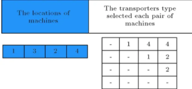
in NSGA-II loop otherwise 4.2.3. Chromosome structure
The proposed chromosome consists of two matrices, each representing a special area of decision making. The rst part shows how machines are placed in locations; the second part represents the allocation of transporters to each pair of machines. Figure 5 shows an example chromosome in which machine 1 is placed in location 1, machine 3 is placed in location 2, machine 2 is placed in location 3, and machine 4 is placed in location 4. The materials between machine 1 and machine 2 are moved by transporter 1, materials between machine 1 and machine 3 are moved by transporter 4, etc.
4.2.4. Crossover operator
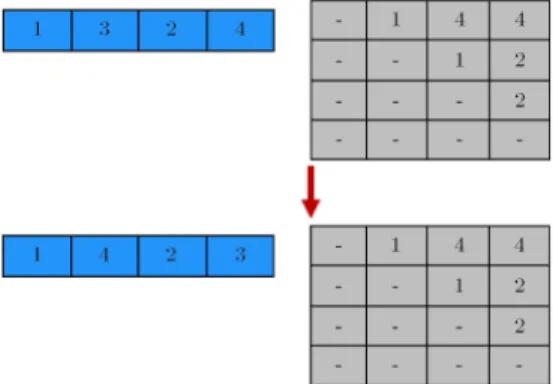
The crossover operator combines two chromosomes to produce a new chromosome. We apply two crossover types that only generate feasible solutions. The rst proposed crossover operator has the following steps;
1. Strings related to machine layout are selected;
2. A cross point is randomly selected (cross points 1; :::; M);
3. The machine numbers before the cross point of parent 1 are copied in the ospring. The remaining machine numbers are put into empty positions according to their relative locations in parent 2.
Figure 6. An example of crossover type 1.
Figure 6 shows the crossover for a problem with 4 machines.
In order to cross the sub-matrices related to transporters, a uniform crossover operator is used in which, rst, a Boolean matrix is generated; then, in cells in which Boolean matrix is equal to one, the data are lled similar to the ospring from parent 1 and in cells in which Boolean matrix is equal to zero, the ospring is lled similar to that from parent 2.
In order to apply the crossover of type 2, a 1 2 reference vector is rst generated. Then, if the rst call of reference vector is 1, the machine layout matrix of ospring will be copied from parent 1; if the rst call of reference vector is 0, the machine layout matrix of ospring will be copied from parent 2. This way is repeated for transporters matrix (Figure 7).
4.2.5. Mutation
In this paper, the mutation operation is performed only on the machine layout matrix. First, a chromosome is randomly selected. Then, to create a hard change, the genes of the selected chromosome are arranged inversely (Figure 8).
4.2.6. The neighbourhood structure
2-change neighborhood is used to dene the neighbor-hood in the local search algorithm. First, we select
Figure 7. An example of crossover type 2.
Figure 8. An example of mutation operator.
Figure 9. An example of neighborhood operator.
a sub-matrix randomly. Then, two dierent cells are selected randomly and the numbers in these cells are exchanged. Figure 9 shows a neighborhood in which sub-matrix 1 changes in genes 2 and 4.
4.2.7. Cooling schedule
The performance of this algorithm also depends on the cooling schedule, which is relevant to the temperature updating function. In the proportional decrement scheme, temperature decreases at steps k and k + 1 of the outer loop by:
Tk+1= Tk; (13)
where is the cooling rate and is obtained by some experiments.
4.2.8. Stopping criterion
To limit the number of replications of both NSGA-II and SA algorithms, some convergence experiments are performed and the best criterion is applied as follows.
NSGA-II will be stopped in the case when total number of iterations reaches a predened number that is set according to the result of experimental design. For stopping SA in a temperature level, rst, we dene the set of m iterations as a round. If the mean change between two successive rounds remains xed within 0.95% condence interval, we reduce the temperature. For the outer loop of SA, a certain number of iterations is set as the stopping criterion, and this value is determined according to the result of experiment.
5. Computational experiments
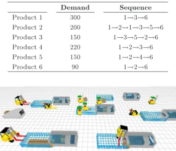
To demonstrate and validate the simulation-based op-timization framework proposed in this paper, a real-life production system is studied. This case study involves 6 machines, named M1, M2, M3, M4, M5, and M6, and 6 products. The demand of product is known (Table 1) and so the material ow between machines is clear. The distance between locations and capacity and speed of the available transporters are, respectively, shown in Tables 2 and 3. The MHC is xed at 1 $/meter. The model is coded in Enterprise
Table 1. Demand rate of products (per day).
Demand Sequence
Product 1 300 1!3!6
Product 2 200 1!2!1!3!5!6
Product 3 150 1!3!5!2!6
Product 4 220 1!2!3!6
Product 5 150 1!2!4!6
Product 6 90 1!2!6
Figure 10. Representation of the real production system in ED simulation software.
Dynamics 8 developer (ED). A graphical representation of the system is shown in Figure 10.
The computational experiments are accomplished in three phases. In the rst phase, we validate the simulation model through real data analysis. In the second phase, an ANN is developed and its accuracy in predicting the makespan is investigated. In the last phase, a comparison between H-NSGA optimization based on articial neural networks and normal optimization based on articial neural networks is presented. The metaheuristic optimization algorithms are coded by MATLAB and are implemented in a desk-top with a 3.20-GHz CPU running Windows 7 (64 bit). 5.1. Simulation model validation
In this section, we investigate whether the simulation model behaves in accordance with the actual system or not. To assess this, simulation results of 30 days are compared with the actual measurement data in terms of makespan for each day. The results are presented in Table 4. As presented in this table, there is an error less than 2%, showing high accuracy of the designed simulation model.
5.2. Developing an articial neural network In this section, a set of proper scenarios are selected for the proposed simulation model to generate training
Table 3. Travel path distance between locations (meter).
From/to 1 2 3 4 5 6
1 0 10 20 15 20 30
2 10 0 10 20 15 20
3 20 10 0 25 20 15
4 15 20 25 0 10 20
5 20 15 20 10 0 10
6 30 20 15 20 10 0
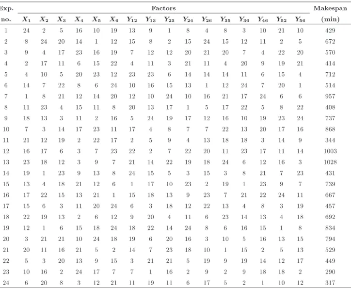
data. Then, a neural network is trained using this data set. Finally, some validation tests are conducted and the ability of designed ANN to predict the makespan is investigated. In this case, there are 16 factors, including 6 factors related to machines' location, each in 6 levels, and 10 factors related to transporters selection, each in 4 levels. The total number of possible experiments is 66 104, which is so computationally
intractable. To overcome this problem, the cong-uration of all experiments is generated by Uniform Design (UD). UD was proposed by Fang [29]. Its most important feature is that it decreases the number of experimental congurations, especially when the experimental region has many factors and multiple levels. According to the uniform design table of the form Un(616), the number of experiments can be
in the range of 17 to 30 (n is the desired number of experiments). Because n should be the common multiple of all the levels of factors, it can only be 24. Therefore, the uniform design table U24, shown in
Table A.1 in Appendix A, is selected. In Appendix A, for factors 1-6 (machines location) the numbers from 1 to 4 signal location 1, the numbers from 5 to 8 signal location 2, etc. For factors 7-16 (transporters selection), the numbers from 1 to 6 signal transporters type 1, the numbers from 7 to 12 signal transporters type 2, etc. The simulation results of all 24 experiments are presented in Appendix A.
The present problem had 16 control factors as the input neurons, and the makespan as the single output. Thus, our ANN includes 16 input nodes and one output node. The number of nodes in the hidden layer can be estimated by Eq. (14) proposed by Chen and Yang [30]:
h = i + o 2 +
p
N; (14)
where i is the number of input nodes, o is the number
Table 2. Characteristics of the transporters. Capacity Speed (m/s) Fixed
cost ($)
No of available transporters
Transporter 1 10 Normal (3,0.5) 500 4
Transporter 2 15 Normal (7,2) 700 3
Transporter 3 10 Normal (3,1) 450 5
Table 4. Results of real system and simulation model. Days Obtained makespan
% Error
no. (minute)
Real system Simulation
1 387 389 0.52
2 340 347 2.06
3 390 401 2.82
4 395 386 2.28
5 384 394 2.60
6 364 383 5.22
7 400 397 0.75
8 400 407 1.75
9 386 393 1.81
10 342 348 1.75
11 399 390 2.26
12 358 355 0.84
13 352 348 1.14
14 396 391 1.26
15 388 394 1.55
16 382 378 1.05
17 340 351 3.24
18 383 391 2.09
19 375 379 1.07
20 342 347 1.46
21 391 380 2.81
22 363 372 2.48
23 388 393 1.29
24 356 370 3.93
25 367 371 1.09
26 399 411 3.01
27 368 361 1.90
28 372 374 0.54
29 385 382 0.78
30 378 387 2.38
Average 375 379 1.92
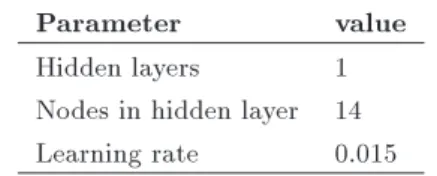
Table 5. The optimal ANN parameters.
Parameter value
Hidden layers 1 Nodes in hidden layer 14 Learning rate 0.015
of output nodes, N is the number experiments, and h is the number of nodes in the hidden layer. Consequently, h = 16+1
2 +
p
24 14. The optimal ANN conguration, which was found experimentally, is summarized in Table 5.
After determining the structure of ANN, back-propagation algorithm is carried out to train the network. The back-propagation algorithm has power-ful approximation capacity and is applicable to both binary and continuous inputs. The type of transfer function employed in this work is a sigmoid function (Eq. (15)) at hidden layer and a linear transfer function at output layer. Neural Network Toolbox V4.0 of MAT-LAB mathematical software was used for makespan prediction:
f(x) = 1 + e1 x: (15) For inter-comparisons between the simulated and mea-sured makespans using the ANN model, two perfor-mance measures, i.e. the Root Mean Squared Error (RMSE) and coecient of determination (R2), are used
as follows [31]:
RMSE = m1 v u u tXM
i=1
Yi Yi
Yi
2
(16)
where m is the number of samples, Yi is the actual
response of sample i, and ^Yi is the predicted response
of sample i. According to RMSE = 0.01545 and R2=
0:9771, the ANN model has been properly trained and has good quality predictions.
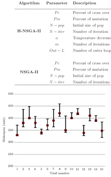
Usually, it is necessary to check the tted model to ensure that it provides an adequate approximation to the new input data. To this aim, the ANN results are compared with respect to their deviations from the simulation results for 15 new trials, which do not belong to the training data set. We propose the condence intervals to evaluate the overall performance of the neural network, because interval estimates are much more useful than point estimates for decision-making. Each trial is simulated for 10 replications and E(Ysim) and V AR(Ysim) are combined to form
condence intervals for each trial (Eq. (17)): Interval = E(Ysim) t
2;r r
p
V AR(Ysim): (17)
As show in Figure 11, in each experiment trail, the predicted result by ANN (red points) falls within the interval obtained by the simulation, and so the capabilities of structured ANN will be proven.
5.3. Evaluation of the proposed metaheuristic algorithm
We tested the optimization framework on numerous random data sets that dier with respect to input parameters such as products demand, transporters capacity, material handling costs, etc. The main challenge in comparing the two multi-objective algo-rithms is that they do not try to nd one optimal solution, but a set of Pareto solutions. A good
Table 6. The parameters of the algorithms and their levels.
Algorithm Parameter Description Low
level
High level
Optimum level
H-NSGA-II
P c Percent of cross over 0.6 0.9 0.85
P m Percent of mutation 0.05 0.15 0.08
N pop Initial size of pop 50 150 130
N iter Number of iteration 50 300 230
Temperature decrement rate 0.96 0.99 0.985
m Number of iterations inside each inner loop 5 30 20 Out L Number of outer loop iterations 50 200 127
NSGA-II
P c Percent of cross over 0.6 0.9 0.80
P m Percent of mutation 0.05 0.15 0.14
N pop Initial size of pop 50 150 140
N iter Number of iterations 50 300 260
Figure 11. Comparison of the results obtained by simulation and ANN model.
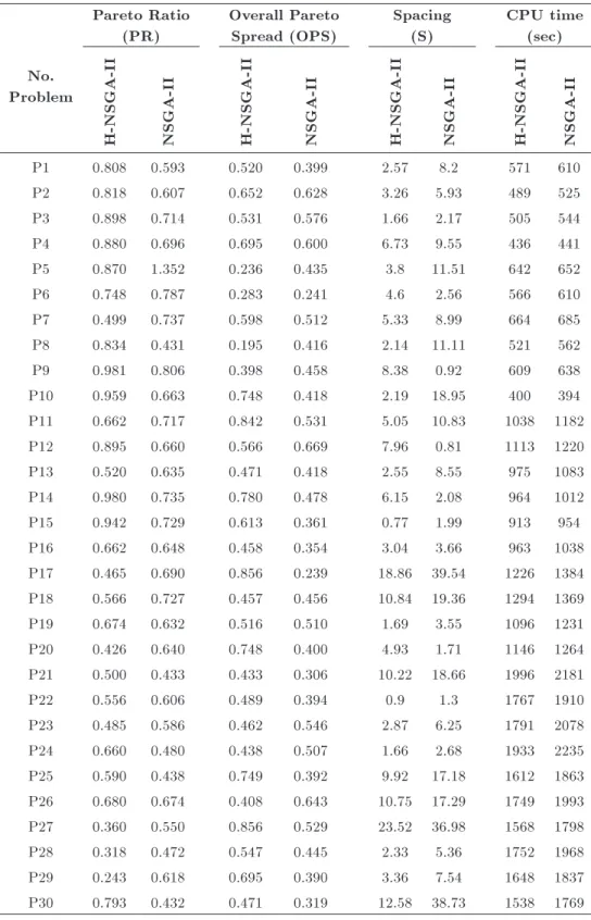
Pareto front is characterized by (i) converging to the real Pareto-optimal front, and (ii) maximizing the diversity of the Pareto solutions. Consequently, the quality of multi-objective optimization algorithms is often dicult to dene precisely by any single performance metric. A list of indicators has been introduced over the past few decades. To analyze the performance of the H-NSGA-II, we compare its Pareto fronts with those obtained by common NSGA-II in terms of metrics Pareto Ratio (PR), Spacing (S), Overall Pareto Spread (OPS), and Computational time (CPU time). PR is the ability of a multi-objective optimization method to produce non-dominated so-lutions. S measures the standard deviation of the distances among solutions of the Pareto front. The smaller the value of the spacing metric, the better are the solutions spread along the obtained front. OPS quanties how widely the non-dominated solutions
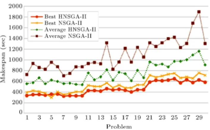
Figure 12. Performance of the algorithms in terms of MHC.
spread over the objectives pace considering all the objectives.
Before evaluating the algorithms, both algorithms are tuned by response surface methodology. The explored bound and optimum level of each parameter are presented in Table 6. Then, the parameters of the algorithms are xed to their optimum level and test problems are solved by the algorithms. Figures 12 and 13 present the results of the proposed H-NSGA-II and normal NSGA-H-NSGA-II in the context of MHC and makespan. As shown in Figure 12, in terms of the best MHC index, H-NSGA-II outperforms NSGA-II in all the test problems, except for P6. Also, in terms of the best makespan, H-NSGA-II nds better results than NSGA-II in all problems, except for P5 (Figure 13). Furthermore, the average values for both objectives considerably improve with the introduction of the adaptive scheme. We also analyze the performances of the algorithms using statistical tests.
Appendix B highlights the values of PR, S, OPS, and CPU time performance measures. As discussed above, these scales are used to measure convergence
Figure 13. Performance of the algorithms in terms of makespan.
and diversity of Pareto-front for handling multiple objectives. As presented in Appendix B, the H-NSGA-II approach with adaptive local search shows better behavior than the approach without local search. In order to statistically analyze the results shown in Appendix B, we use Student's t-test. The hypothesis is:
H0: 1 2= 0;
H1: 1 26= 0;
in which 1is the obtained average value by
H-NSGA-II and 2 is the obtained value by NSGA-II algorithm.
The results are shown in Table 7. According to Table 7, it can be seen that in terms of PR and CPU time index, there is no meaningful dierence between algorithms. But, H-NSGA-II outperforms NSGA-II with respect to spacing and OPS metrics. The last column of Table B.1 in Appendix B shows the computational times of the algorithms for each test problem. Although there was no signicant CPU time dierence between algorithms, according to \Mean" statistics, it can be claimed that H-NSGA-II is relatively faster than NSGA-II. This statement implies that although embedding the SA in
some generations of NSGA-II may lead to increase in computational time, large increase in solution quality and speed of convergence can compensate it.
6. Conclusion and remarks
This paper presents a new model and a novel solving approach to solve facility layout optimization problems for manufacturing systems with dynamic character-istics. The proposed approach integrates computer simulation, ANN, and H-NSGA-II techniques to over-come the limitations of traditional layout optimization methods. The main motivation behind choosing this problem is the necessity for integrating decisions for the layout of machines and material handling vehicles. The results show that the application of an ANN model can predict the makespan in a complicated manufacturing system, eciently. Despite the previous models, this paper considers real aspects of material handling such as random breakdowns, random processing times, and waiting times during the handling process. Since these aspects are stochastic variables and theoretically dicult to obtain, the ANN model, which has been trained by the simulation model results, computes the problem makespan.
In the experimental results, there were 66
alterna-tives for the layout of machines and 104alternatives for
selecting the transporters; therefore, there were a total number of 66104designs. However, in the experiment,
only 24 simulation congurations were run to train the data set needed for ANN model. A case study was presented and the simulation results were given for validation of the ANN results. In all experiments, the ANN precision was 95%. Finally, a hybrid non-dominated sorting genetic algorithm was proposed to search the solution space. The performance of the proposed algorithm was compared with that of the normal non-dominated sorting genetic algorithm. In terms of PR and CPU time criteria, both algorithms
Table 7. Results of two-sample T -test.
Source No Mean St. Dev 95% CI for dierence T -Value P -Value PR H-NSGA-II 30 0.676 0.206 (-0.0697, 0.1217) 0.54 0.588
NSGA-II 30 0.650 0.168
OPS H-NSGA-II 30 0.557 0.177 (0.0282, 0.1812) 2.75 0.008
NSGA-II 30 0.452 0.110
Spacing H-NSGA-II 30 6.02 5.33 (-9.29, -0.27) -2.14 0.038
NSGA-II 30 10.8 11.0
CPU time H-NSGA-II 30 1116 511 (-405, 169) -0.82 0.413
performed similar. But, in terms of OPS and spac-ing metric criteria, the performance of the proposed hybrid algorithm was statistically better. For future research, one may extend unequal area constraint of departments, which demonstrates a more realistic representation of real-world manufacturing facilities. Also, other factors aecting the makespan, such as human factors, can be investigated.
References
1. Singh, S.P. and Sharma, R.R.K. \A review of dierent approaches to the facility layout problems", Int. J. Adv. Manuf. Technol., 30, pp. 425-433 (2006). 2. Tompkins, J.A., White, J.A., Bozer, Y.A. and
Tan-choco, J.M.A., Facilities Planning, Wiley, New York (2003).
3. Meller, R.D. and Gau, K.Y. \The facility layout prob-lem: Recent and emerging trends and perspectives", J. Manuf. Syst., 15(5), pp. 351-366 (1996).
4. Azadivar, F. and Wang, J. \Facility layout optimiza-tion using simulaoptimiza-tion and genetic algorithms", Int. J. Prod. Res., 38(17), pp. 4369-4383 (2000).
5. Egbelu, P.J. and Tanchoco, J.M.A. \Potentials for bi-directional guide-path for automated guided vehicle based systems", Int. J. Prod. Res., 24(5), pp. 1075-1097 (1986).
6. Rosenblatt, M.J. \The facilities layout problem: A multi-goal approach", Int. J. Prod. Res., 17(4), pp. 323-332 (1979).
7. Savsar, M. \Flexible facility layout by simulation", Comput. Ind. Eng., 20(1), pp. 155-165 (1991). 8. Morris, J.S. and Tersine, R.J. \A simulation
compari-son of process and cellular lay-outs in a dual resource constrained environment", Comput. Ind. Eng., 26(4), pp. 733-41 (1994).
9. Pagell, M. and Melnyk, S.A. \Assessing the impact of alternative manufacturing layouts in a service setting", J. Oper. Manage., 22(4), pp. 413-29 (2004).
10. Zhou, F., AbouRizk, S.M. and AL-Battaineh, H. \Optimization of construction site layout using a hy-brid simulation-based system", Simul. Modell. Pract. Theory, 17, pp. 348-363 (2009).
11. Jithavech, I. and Krishnan, K.K. \A simulation-based approach for risk assessment of facility layout de-signs under stochastic product demands", Int. J. Adv. Manuf. Technol., 49(1), pp. 27-40 (2009).
12. Gupta, R.M. \Flexibility in layouts: A simulation approach", Material Flow., 3, pp. 243-250 (1986). 13. Grajo, E.S. \Strategic layout planning and simulation
for lean manufacturing a layOpt tutorial", Proceedings of the 1996 Winter Simulation Conference, pp. 564-568 (1996).
14. Azadivar, F. and Tompkins, G. \Simulation optimiza-tion with quantitative variables and structural model
changes: a genetic algorithm approach", Eur. J. Oper. Res., 113, pp. 169-182 (1999).
15. Kulturel-Konak, S., Smith, A.E. and Norman, B.A. \Layout optimization considering production uncer-tainty and routing exibility", Int. J. Prod. Res., 42(21), pp. 4475-4493 (2004).
16. Altuntas, S. and Selim, H. \Facility layout using weighted association rule-based data mining algo-rithms: Evaluation with simulation", Expert Syst. Appl., 39, pp. 3-13 (2012).
17. Dombrowski, U. and Ernst, S. \Scenario-based simula-tion approach for layout planning", 8th CIRP Conf. on Intell. Comput in Manuf. Eng., 12, pp. 354-359 (2013). 18. Karpe, A.B., Kulkarni, C.N. and Jahagirdar, R.S. \Simulation methodology for facility layout problems", Int. J. Res. Eng. Sci. Technol., 1, pp. 1-10 (2011). 19. Azadeh, A., Nazari, T. and Charkhand, H.
\Opti-mization of facility layout design problem with safety and environmental factors by stochastic DEA and simulation approach", Int. J. Prod. Res., 1(1), pp. 12-17 (2014).
20. Chiang, W., Kouvelis, P. and Urban, T. \Single and multiobjective facility layout with workow interfer-ence considerations", Eur. J. Oper. Res., 174(3), pp. 1414-1426 (2006).
21. Fu, M.C. \Optimization for simulation: Theory vs. practice", Inf J. Comput., 14, pp. 192-215 (2002). 22. Wang, G., Yan, Y., Zhang, X., Shangguan, J. and
Xiao, Y. \A simulation optimization approach for facility layout problem", Proc. of the IEEE Int'l. Conf. on Ind. Eng. Eng. Manage., pp. 734-738 (2008). 23. Swisher, J.R., Hyden, P.D., Jacobson, S.H. and
Schruben, L.W. \A survey of recent advances in discrete input parameter discrete-event simulation op-timization", IIE Trans., 36, pp. 591-600 (2004). 24. Fu, M.C., Glover, F.W. and April, J. \Simulation
optimization: a review, new developments, and appli-cations", In: Kuhl ME, Steiger NM, Joines JA, Eds., Proceedings of the 2005 Winter Simulation Conference (2005).
25. Ashtiani, A., Mirzaei, P.A. and Haghighat, F. \Indoor thermal condition in urban heat island: Comparison of the articial neural network and regression methods prediction", Energy Build., 76, pp. 597-604 (2014). 26. Funahashi, K. \On the approximate realization of
continuous mappings by neural networks", Neural Netw., 2(1), pp. 83-92 (1989).
27. Hornik, K., Stinchcombe, M. and White, H. \Multi-layer feed forward networks are universal approxima-tors", Neural Netw., 2, pp. 359-66 (1989).
28. Deb, K., Pratap, A., Agarwal, S. and Meyarivan, T. \A fast and elitist multiobjective genetic algorithm: NSGA-II", IEEE Trans. Evol. Comput., 6, pp. 182-197 (2002).
29. Fang, K.T. \The uniform design: application of number-theoretic methods in experimental design", Acta Math. Appl. Sin., 3, pp. 363-372 (1980).
30. Chen, M.C. and Yang, T. \Design of manufacturing systems by a hybrid approach with neural network meta modelling and stochastic local search", Int. J. Prod. Res., 40, pp. 71-92 (2002).
31. Geyikci, F., Kilic, E., Coruh, S. and Elevli, S. \Model-ing of lead adsorption from industrial sludge leachate on red mud by using RSM and ANN", Chem. Eng. J., 183, pp. 53-59 (2012).
Appendix A
The uniform design of experiments is shown in Table A.1.
Appendix B
The multi objective performance measures obtained for the algorithms is shown in Table B.1.
Biographies
Parham Azimi was born in 1974. He received his BS, MS, and PhD degrees in Industrial Engineering from Sharif University of Technology in 1996, 1998, and 2005, respectively. Currently, he is the Assistant Professor of Industrial Engineering at Islamic Azad University (Qazvin Branch). His research interests include optimization via simulation techniques, facility layout problems, location allocation problems, graph theory, and data mining techniques.
Parham Soo Parham Soo is a PhD candidate at the Faculty of Industrial and Mechanical engineering, Azad university, Qazvin branch. His research elds are MCDM and Simulation optimization. He has been also a project manager at the Iranian Fuel Conservation Organization for designing and production of 500,000 pcs. of CNG valves and also exporting of LPG valves to the European markets including Germany and the Netherlands.
Table A.1. Uniform design of experiments.
Exp. Factors Makespan
no. X1 X2 X3 X4 X5 X6 Y12 Y13 Y23 Y24 Y26 Y35 Y36 Y46 Y52 Y56 (min)
1 24 2 5 16 10 19 13 9 1 8 4 8 3 10 21 10 429
2 8 24 20 14 1 12 15 8 2 15 24 15 12 11 2 5 672
3 9 4 17 23 16 19 7 12 12 20 21 20 7 4 22 20 570
4 2 17 11 6 15 22 4 11 3 21 11 4 20 9 19 21 414
5 4 10 5 20 23 12 23 23 6 14 14 14 11 6 15 4 712
6 14 7 22 8 6 24 10 16 15 13 1 12 24 7 20 1 514
7 1 8 21 12 14 20 12 10 24 10 16 21 17 24 6 6 957
8 11 23 4 15 11 8 20 13 17 1 5 17 22 5 8 22 408
9 18 13 3 11 2 16 5 24 19 17 12 16 10 19 23 24 737
10 7 3 14 17 23 11 17 4 8 7 7 22 13 20 17 16 868
11 21 12 19 2 22 17 2 5 9 4 13 18 18 3 14 9 344
12 16 17 6 3 7 23 22 2 7 22 20 11 23 17 11 14 1003
13 23 18 12 3 9 7 21 14 22 19 18 24 6 12 16 3 1028
14 19 1 23 9 13 8 24 15 5 3 15 3 8 21 7 23 431
15 13 4 18 21 12 6 1 17 10 23 2 19 1 23 9 7 739
16 17 22 15 13 21 1 15 18 13 9 23 7 21 22 24 11 667
17 15 6 3 11 20 24 6 3 18 12 22 13 4 8 3 19 457
18 22 19 13 2 6 12 9 20 4 11 6 23 14 13 4 18 692
19 12 1 6 15 18 24 18 22 14 24 8 6 16 15 1 8 834
20 3 21 21 10 24 18 19 6 20 16 3 10 5 16 13 15 794
21 20 11 16 21 5 2 14 7 23 18 10 1 15 2 5 13 529
22 5 3 20 13 9 15 3 21 21 5 19 9 19 14 12 17 449
23 10 16 2 24 17 7 7 1 16 2 9 2 9 18 18 2 290
Table B.1. Multi-objective performance measures obtained for the algorithms.
No. Problem
Pareto Ratio (PR)
Overall Pareto Spread (OPS)
Spacing (S)
CPU time (sec)
H-NSGA-I
I
NSGA-I
I
H-NSGA-I
I
NSGA-I
I
H-NSGA-I
I
NSGA-I
I
H-NSGA-I
I
NSGA-I
I
P1 0.808 0.593 0.520 0.399 2.57 8.2 571 610
P2 0.818 0.607 0.652 0.628 3.26 5.93 489 525
P3 0.898 0.714 0.531 0.576 1.66 2.17 505 544
P4 0.880 0.696 0.695 0.600 6.73 9.55 436 441
P5 0.870 1.352 0.236 0.435 3.8 11.51 642 652
P6 0.748 0.787 0.283 0.241 4.6 2.56 566 610
P7 0.499 0.737 0.598 0.512 5.33 8.99 664 685
P8 0.834 0.431 0.195 0.416 2.14 11.11 521 562
P9 0.981 0.806 0.398 0.458 8.38 0.92 609 638
P10 0.959 0.663 0.748 0.418 2.19 18.95 400 394
P11 0.662 0.717 0.842 0.531 5.05 10.83 1038 1182
P12 0.895 0.660 0.566 0.669 7.96 0.81 1113 1220
P13 0.520 0.635 0.471 0.418 2.55 8.55 975 1083
P14 0.980 0.735 0.780 0.478 6.15 2.08 964 1012
P15 0.942 0.729 0.613 0.361 0.77 1.99 913 954
P16 0.662 0.648 0.458 0.354 3.04 3.66 963 1038
P17 0.465 0.690 0.856 0.239 18.86 39.54 1226 1384 P18 0.566 0.727 0.457 0.456 10.84 19.36 1294 1369
P19 0.674 0.632 0.516 0.510 1.69 3.55 1096 1231
P20 0.426 0.640 0.748 0.400 4.93 1.71 1146 1264
P21 0.500 0.433 0.433 0.306 10.22 18.66 1996 2181
P22 0.556 0.606 0.489 0.394 0.9 1.3 1767 1910
P23 0.485 0.586 0.462 0.546 2.87 6.25 1791 2078
P24 0.660 0.480 0.438 0.507 1.66 2.68 1933 2235
P25 0.590 0.438 0.749 0.392 9.92 17.18 1612 1863
P26 0.680 0.674 0.408 0.643 10.75 17.29 1749 1993 P27 0.360 0.550 0.856 0.529 23.52 36.98 1568 1798
P28 0.318 0.472 0.547 0.445 2.33 5.36 1752 1968
P29 0.243 0.618 0.695 0.390 3.36 7.54 1648 1837
![Figure 1. Solution to the eight-facility example: (a) Minimizing MHC, and (b) minimizing work
ow interference [20].](https://thumb-us.123doks.com/thumbv2/123dok_us/8379957.2226185/3.892.447.809.434.1105/figure-solution-facility-example-minimizing-mhc-minimizing-interference.webp)