Sharif University of Technology
Scientia IranicaTransactions E: Industrial Engineering www.scientiairanica.com
Research Note
Modeling and optimization of the multi-objective
single-buyer multi-vendor integrated inventory problem
with multiple quantity discounts
A. Kamali
a, S.M.T. Fatemi Ghomi
a;and F. Jolai
ba. Department of Industrial Engineering, Amirkabir University of Technology, 424 Hafez Avenue, Tehran, 1591634311, Iran. b. Department of Industrial Engineering, College of Engineering, University of Tehran, Tehran, Iran.
Received 8 June 2015; received in revised form 4 December 2015; accepted 25 April 2016
KEYWORDS Integrated inventory; Multi-vendor; Multiple discounts; Multi-objective.
Abstract. This paper deals with a multi-objective integrated inventory model to coordinate a two-stage supply chain including a single buyer and multiple vendors. The earlier work on the problem is limited to considering only one type of discount. This paper extends the problem under the multiple quantity discount environment. We try to minimize the system cost, number of defective items, number of late delivered items and maximize the total purchasing value. Numerical examples are presented to provide some insights into the proposed model and dierent discount schemes. Results obtained from sensitivity analysis show that changes in unit prices have a relatively large eect on the objective function; as the upper bounds of discount intervals are reduced, the value of objective function decreases. It is also seen that the order quantity from the suppliers increases as the number of suppliers oering all unit quantity discounts increases. In addition, we use a solution approach that is not used by previous studies on this problem, and the obtained results show that the DE algorithm, proposed in this study, outperforms the PSO proposed by Kamali et al. [1] in both solution quality and computational time.
© 2017 Sharif University of Technology. All rights reserved.
1. Introduction
With the growing focus on supply chain management, companies are pushed towards a close collaboration with their suppliers and customers. Researchers have studied dierent features of the supply chain coordina-tion in recent years. Coordinacoordina-tion models are presented to improve the overall performance of the supply chain by considering the benets of all the members of the supply chain. In the case of one buyer and multiple
*. Corresponding author. Tel.: +98 21 88021067; Fax: +98 21 88013102
E-mail addresses: amir [email protected] (A. Kamali); [email protected] (S.M.T. Fatemi Ghomi); [email protected] (F. Jolai)
vendors, the goal is to determine one or more vendors and allocate the order quantities to them, such that the eciency of the entire system, consisting of buyer and vendors, is improved.
This paper considers the issue of coordination between one buyer and multiple potential suppliers in the supplier selection process. Quantity discount policies are used as common incentives from vendors to motivate the buyer to participate in the coordination. In this paper, quantity discounts are used to encourage the coordination. In this way, while the vendors benet from the integrated model, quantity discounts oered by the vendors can encourage the buyer to participate in the coordination. As an example of this type of supply chain, we can mention the production pat-terns in steel, chemical, petrochemical, and electronic
industries where the upstream stage, with multiple production lines in parallel, produces a single product and feeds the outputs to the downstream stage [2]. For example, in the steel industry, several lines produce slabs in parallel and feed them to a rolling mill. In these situations, the problem of determining the right suppli-ers and allocating the required quantity to the selected suppliers arises. Another area of the problem is that our model may be applied to the automotive industry where buyers and vendors engage in strategic partner-ships with the intention to create competitive advan-tages. In this case, using an integrated inventory model may help to coordinate material ows in the system [3]. Regarding the related recent studies to this work, Tabrizi el al. [4] considered a robust discount scheme that can be incorporated into this study as a future research. Giri and Chakraborty [5] considered a multi-supplier multi-buyer problem with stochastic demand and only one objective function maximizing the ex-pected prot of the system. Kundu and Jain [6] developed a smart decision support system providing solutions for power dierence issues amongst supply chain partners for a single-product N-supplier system. Adeinat and Ventura [7] considered capacity and quan-tity restrictions on the problem. A supplier selection model in a make-to-order environment considering quantity discount was studied by Guan et al. [8]. They employed a multi-objective approach. In another work, Kermani et al. [9] considered a supplier selection problem with price, quality, and delivery performance criteria, but in a single-echelon supply chain, each manufacturer only tries to optimize his/her position while deteriorating other buyers' situation. Chen and Sarker [10] studied an integrated inventory lot-sizing and vehicle routing problem focusing on sup-plier/manufacturer cooperation in a JIT system with multi-supplier and single-assembler. Kamali et al. [1] developed a multi-objective single-buyer multi-vendor supply chain coordination model which considered the all-unit quantity discount policy for the vendors. They proposed a Particle Swarm Optimization (PSO) algorithm and a Scatter Search (SS) algorithm to simul-taneously determine the number of suppliers to employ and the order quantity allocated to these suppliers.
Furthermore, in this paper, we propose a Dieren-tial Evolution (DE) algorithm to solve the current NP-hard problem. In this regard, studies of Shaeezadeh and Sadeghieh [11], Wang et al. [12], Shahparvari et al. [13], and Lo [14] are instances of the recent studies employing single and multi-objective dieren-tial evolution algorithms for inventory problems in the supply chain. In order to enhance the performance of the proposed algorithms, we apply a local search procedure. Furthermore, we adopt a repair algorithm for constraint handling within the proposed algorithms. The performance of the proposed algorithm is
evalu-ated by comparing its results with the PSO algorithm proposed by Kamali et al. [1]. The obtained results are also compared with the exact optimal solutions to small-sized problems.
The earlier work of Kamali et al. [1] is limited to considering only one type of discount. However, it is obvious that in practical situations, buyers face with multiple-sourcing in which suppliers may oer dierent price discount schemes [15]. Thus, in this paper, to capture a more practical situation, we extend the model to consider both types of quantity discount at the same time: all-unit discount and incremental discount. Here, we address the issue of coordination of a single-buyer multi-vendor supply chain in an integrated inventory model where each vendor can oer one of the two discount schemes, i.e. all-unit discount and incremental discount, on the unit price of the item. Considering both types of quantity discount and both quantitative and qualitative criteria in the model, it is made to be more practical as compared to that of other previous studies. In addition, we investigate the eect of the number of suppliers oering all-unit quantity discount on the values of the objective functions, providing some insights into the proposed model. Moreover, we use a solution approach to this problem that is not used by previous studies, and the obtained results show that the DE algorithm, proposed in this study, outperforms the PSO proposed by Kamali et al. [1] in both solution quality and computational time.
The paper is organized as follows. In Section 2, the problem is dened, its assumptions are described, and its mathematical modeling is presented. The procedure to solve the problem is discussed in Section 3. In Section 4, a numerical example is presented to evaluate the results obtained from the proposed model. In Section 5, some experimental designs are presented. Finally, Section 6 is dedicated to the summary and conclusion of the paper.
2. Problem denition and formulation
Consider a system in which a single buyer is going to purchase the annual required quantity of a single item or product from the multiple vendors. Buyer's demand is known with a predetermined annual rate (D); each vendor (indexed by i) is assumed to have a nite production rate (Pi). The vendors are also supposed
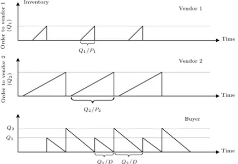
to have dierent quality and delivery performances in terms of percentage of defective items and percentage of late delivery items, respectively. In this paper, two types of quantity discounts, all-unit discount and incremental discount, are considered, and each vendor can adopt one of the two quantity discount policies. In this problem, it is assumed that, in each period, after all ith vendor's order quantities are consumed, (i+1)th vendor's order quantity can be entered. Figure 1
Figure 1. Inventory levels for two vendors and a single buyer.
depicts the inventory levels of the buyer and two vendors for the considered delivery structure. The aim of the model is to determine one or more vendors and allocate the order quantities to them. In the following, four objectives are considered in the modeling of the problem: 1) minimizing the total cost of the supply chain including vendors' annual cost and buyer's an-nual cost; 2) minimizing the total number of defective items; 3) minimizing the total number of late delivery items; and 4) maximizing the total purchasing value. Parameters
i Index of vendors
k Index of discount intervals n Total number of vendors
Ki Index of the last discount interval
oered by the ith vendor
n1 Number of vendors oering all-unit
quantity discount
uik The upper bound of the kth discount
interval oered by the ith vendor u
ik Slightly smaller than uik
cik Unit price of the product for the kth
discount interval oered by the ith vendor
di Percentage of defective items for the
ith vendor
li Percentage of late delivery items for
the ith vendor
wi Total performance (weight) of the ith
vendor in qualitative criteria D Annual demand rate of the buyer Ai Fixed/order cost for the ith vendor
Si The ith vendor's setup cost
Pi Annual production rate of the ith
vendor
zi Unit production variable cost for the
ith vendor
hb The buyer's holding cost per unit per
unit time
hi The ith vendor's holding cost per unit
per unit time Decision variables
qik Amount of the products ordered to the
ith vendor at the kth discount interval yik Binary variable; if the order quantity
from the ith vendor falls at the kth interval, then yik = 1; otherwise,
yik= 0
Dependent variables
Qi Amount of the products ordered to the
ith vendor (Qi=PKk=1i qik)
Q Total order quantity from all vendors (Q =Pni=1Qi)
CPb Annual purchasing cost of the buyer
CPi Annual production cost of the ith
vendor
CAb Annual ordering cost of the buyer
CSi Annual setup cost of the ith vendor
CHb Annual holding cost of the buyer
CHi Annual holding cost of the ith vendor
T C(b) Total annual cost of the buyer T C(v) Total annual cost of the vendors T C Total cost of the supply chain
2.1. Cost function
The total annual cost of the supply chain, which includes the annual cost of the buyer and the annual cost of the vendors, is calculated as follows.
2.1.1. The buyer's total cost
The total annual cost of the buyer is:
T C(b) = CPb+ CAb+ CHb; (1)
CPb depends on the unit price of item, which is oered
in the following two discount schemes: all-unit discount and incremental discount. Supposing that n1vendor(s)
oer all-unit discount, the number of vendor(s) who oers incremental discount is n n1.
Under all-unit quantity discount policy, the unit cost corresponding to the size of the order is applied to the all-units of order. Hence, CPb under all-unit
discount policy can be modeled as: D Q n1 X i=1 Ki X k=1
cikqik; (2)
where D
Q represents the number of periods in the time
horizon, ci1 > ci2> ::: > ciKi, and at most one of the
variables qikfor 8k, k = 1; 2; :::; ki, can be positive and
the rest are equal to zero.
Under incremental quantity discount policy, a unit price is applied only to the number of units above the breakpoint. CPb under incremental discount policy
can be written as: D
Q
n
X
i=n1+1
Ki
X
k=1
cik(qik yikui;k 1)
+ yik k 1
X
j=1
cij(uij ui;j 1)
; (3)
where ui;0is a positive small value for all vendor, ci1>
ci2 > ::: > ciKi, and at most one of the variables qik
for 8k, k = 1; 2; :::; Ki, can be positive and the rest are
equal to zero. Thus, CPb is obtained as:
CPb =
D Q n1 X i=1 Ki X k=1
cikqik+DQ n
X
i=n1+1
Ki
X
k=1
cik(qik
yikui;k 1) + yik k 1
X
j=1
cij(uij ui;j 1)
=DQ Xn1
i=1 Ki
X
k=1
cikqik+ n
X
i=n1+1
Ki
X
k=1
yik
k 1X
j=1
cij(uij ui;j 1) cikui;k 1
:
(4)
The annual ordering cost of buyer (CAb) is:
CAb=
D Q n X i=1 Ki X k=1
Aiyik: (5)
Referring to Figure 1, the average on hand inventory of the buyer for the ith vendor per unit time is:
Ibi=
Q2 i
2Q = PKi
k=1qik
2
2Q : (6)
Thus, the annual holding cost of the buyer is obtained as:
CHb =
n
X
i=1
hbIbi =
hb 2Q n X i=1 Ki X k=1 qik !2 : (7)
Hence, the total annual cost of the buyer is obtained as:
T C(b) =CPb+CAb+CHb=
D Q n X i=1 Ki X k=1
(cikqik+Aiyik)
+DQ
n
X
i=n1+1
Ki
X
k=1
yik
k 1X
j=1
cij(uij ui;j 1)
cikui;k 1
+2Qhb
n X i=1 Ki X k=1 qik !2 : (8) 2.1.2. The vendors' total cost
The annual production cost and the annual setup cost of the ith vendor are obtained using Eqs. (9) and (10), respectively:
CPi =
D Q
Ki
X
k=1
ziqik; (9)
CSi =
D Q
Ki
X
k=1
Siyik: (10)
According to Figure 1, the average on hand inventory of the ith vendor per unit time is:
Ii= DQ 2 i
2QPi =
D 2Q
PKi
k=1qik
Pi 2
: (11)
Thus, the annual holding cost of the ith vendor is obtained as:
CHi = hiIi=
D 2Q hi Pi n X i=1 Ki X k=1 qik !2 : (12)
Thus, the total annual cost of all vendors becomes:
T C(v) =
n
X
i=1
(CPi+ CSi+ CHi)
=DQXn
i=1 Ki
X
k=1
(ziqik+ Siyik)
+2QD Xn
i=1 hi Pi Ki X k=1 qik !2 : (13)
From Eqs. (8) and (13), the total cost of the supply chain, as the rst objective function, is calculated as:
Z1= T C = T C(b) + T C(v)
=DQ
n X i=1 Ki X k=1
(zi+ cik)qik+ (Ai+ Si)yik
+DQ
n
X
i=n1+1
Ki
X
k=1
yik
k 1X
j=1
cij(uij ui;j 1)
cikui;k 1
+D Q n X i=1 1 2 hb D + hi Pi Ki X k=1 qik !2 : (14) 2.2. Defective items function
In order to improve the product quality and eective-ness of the supply chain, this objective function is applied which minimizes the total number of defective items in the supply chain as follows:
Z2=DQ n X i=1 Ki X k=1
diqik: (15)
2.3. Late delivery function
This objective function minimizes the total number of late delivery items in the supply chain and can be stated as follows:
Z3=DQ n X i=1 Ki X k=1
liqik: (16)
2.4. Total purchasing value function
The Analytical Hierarchy Process (AHP), introduced by Saaty [16], is an eective approach to deal with the multi-criteria problems. By using AHP, the model is enabled to make a trade-o between several tangible and intangible factors with dierent priorities [17]. The main steps of the algorithm are [17]:
1. Dene the criteria for supplier selection;
2. Calculate the weights of the criteria;
3. Rate the alternative suppliers;
4. Compute the overall score of each supplier;
5. Build the linear model and maximize the objective function.
Let wibe the total performance of the ith vendor
in qualitative criteria calculated by AHP. Hence, the total purchasing value, which has to be maximized, is obtained as:
Z4=DQ n X i=1 Ki X k=1
wiqik: (17)
2.5. The constraints
The total annual production quantity of all vendors (D=QPni=1PKi
k=1qik) is equal to the annual demand
rate of buyer (D). Thus, we will have:
n X i=1 Ki X k=1
qik= Q: (18)
The total quantity ordered to the ith vendor (D=QPKi
k=1qik) is equal or less than the production
rate of this vendor (Pi). Hence:
Ki
X
k=1
qik PDi:Q; 8i; i = 1; 2; :::; n: (19)
The discount intervals constraints can be modeled as follows:
qik uikyik; 8i; i = 1; 2; :::; n; 8k; k = 1; 2; :::; Ki;
(20)
qikui;k 1yik; 8i; i=1; 2; :::; n; 8k; k =1; 2; :::; Ki;
(21)
Ki
X
k=1
yik 1; 8i; i = 1; 2; :::; n; (22)
where ui;0is a positive small value for all vendors.
Finally, to satisfy the buyer's demand and due to the fact that phrase Q is the denominator of the fractions in the objective functions, we set Q greater than a small positive value (i.e., Q > ").
2.6. The multi-objective model
The problem can be formulated as a multi-objective mixed integer nonlinear programming model as fol-lows:
Minimize [Z1; Z2; Z3; Z4];
subject to:
n
X
i=1 Ki
X
k=1
qik= Q;
Ki
X
k=1
qikPDi:Q; 8i; i = 1; 2; :::; n;
qikuikyik; 8i; i=1; 2; :::; n; 8k; k =1; 2; :::; Ki;
qikui;k 1yik; 8i; i=1; 2; :::; n; 8k; k =1; 2; :::; Ki; Ki
X
k=1
yik 1; 8i; i = 1; 2; :::; n;
Q > ";
qik 0; 8i; i = 1; 2; :::; n; 8k; k = 1; 2; :::; Ki;
yik2f0; 1g; 8i; i=1; 2; :::; n; 8k; k =1; 2; :::; Ki:(23)
One common approach in dealing with multi-objective problems is to minimize the summation of relative deviations of all objectives from their individual op-timal values [18]. Suppose that the decision-maker assigns relative weight Wi (8i; i = 1; 2; 3; 4) to
the ith objective. The weighted objective func-tion as the summafunc-tion of normalized deviafunc-tion of each objective from its optimal value is established as:
MinimizeZ =W1
Z1 Z1
Z 1
+ W2
Z2 Z2
Z 2
+ W3
Z3 Z3
Z 3
+ W4
Z
4 Z4
Z 4
: (24)
In this formulation, Z
i (8i; i = 1; 2; 3; 4) is the
best value of the ith objective function obtained by optimizing the objective function under the con-straints of the problem ignoring other objective func-tions.
3. The proposed DE algorithm
Burke et al. [19] stated that supplier selection prob-lems under all-unit or incremental quantity discount policies are categorized among the NP-hard problems. There are various evolutionary algorithms to solve the complex problems. Dierential Evolution (DE) is from
the class of population-based evolutionary algorithms, developed by Storn and Price [20], which is a reliable and versatile method and easy to use. Also, DE has been shown to be ecient for global optimization over continuous real spaces [20]. Recently, DE has been used by Qu et al. [21] for solving a stochastic location-inventory problem with two replenishment policies, joint replenishment, and independent replenishment; results show the eectiveness of the algorithm. Wang et al. [22] developed a simple and improved dierential evolution algorithm to solve a procurement approach using the joint replenishment and channel coordination policy in a two-echelon supply chain considering the coordination cost. Also, Cui et al. [23] adopted a dierential evolution algorithm to solve a RFID-based investment evaluation model for the joint replenish-ment and delivery problem under stochastic demand. Hence, we utilize this algorithm to solve the current problem. Furthermore, Kamali et al. [1] showed the good performance of the Particle Swarm Optimization (PSO) in nding the near optimal solutions in a sup-plier selection and coordination problem. Therefore, this paper adopts the same representation and extends it for the current problem.
In DE algorithm, for each individual in the pop-ulation, an ospring is generated using the weighted dierence of parent solutions. Then, the ospring is replaced with the parent if it is tter. Otherwise, the parent retains its place in the population in the next generation. These steps are repeated until the stopping criterion is satised. (See Storn and Price [20] for more details). In the following, the overall structure of the proposed algorithm is presented.
3.1. Overall structure of the proposed DE algorithm
In the considered problem, solution vectors have the following format [1]:
X =
z Q}|1 {
q11; :::; q1;K1;
Q2
z }| { q21; :::; q2;K2; :::;
Qn
z }| { qn1; :::; qn;Kn
: (25) We use an approach to generate the initial solutions and a local search algorithm to enhance the per-formance of the proposed algorithm similar to those implemented by Kamali et al. [1]; readers can refer to this article for more details. Furthermore, during the evolutionary algorithms, solutions may violate the constraints related to the vendors' annual production rate (Constraint (19)), resulting in infeasible solutions. Hence, we employ a procedure to repair generated infeasible solutions [1].
Algorithm 1 describes the overall structure of the proposed DE algorithm. As it can be seen in this algorithm, after initializing target vector Xi, it is
Algorithm 1. The proposed DE algorithm.
is an infeasible solution, repair algorithm is applied to transform it to a feasible solution. Furthermore, in the consecutive iterations, the local search procedure is applied to each trial vector Ui, and if the result is
infeasible, the repair algorithm replaces the infeasible solution with its feasible version.
4. Numerical example
A supply chain system consisting of three suppliers and a single buyer is considered. The buyer's demand is 100000 units per year, and his (her) inventory holding cost per unit per unit time is equal to 3.24. Discount intervals oered by the suppliers are shown in Table 1, and Table 2 gives some other information of the suppliers.
Table 3 shows the obtained results considering W1 = 0:3, W2 = 0:4, W3 = 0:2, and W4 = 0:1 in
dierent levels of n1. As we can see, the order quantity
from the suppliers increases as n1 increases. Table 3
Table 3. Solutions of the example in dierent levels of n1.
n1 = 0 n1= 1 n1= 2 n1 = 3
Z 0.038 0.0412 0.0712 0.0336 Z1 1012483 1012483 993473.3 978223.1
Z2 3600 3600 3600 3600
Z3 28650 28650 28650 28650
Z4 25800 25800 25800 25800
Q1 0 0 0 0
Q2 945 945 4000 6461.5
Q3 1755 1755 7428.6 12000
also indicates that in the nal solutions, Z2and Z3are
in their optimal values, and the values of Z1 and Z4
are worse than their optimal values.
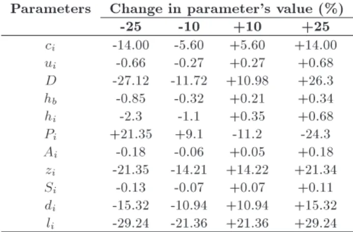
We conduct a sensitivity analysis on the main parameters of the model. Table 4 shows percentage of changes in the associated objective function in levels of -25%, -10%, +10%, and +25% changes in the value of each parameter. We can see from the table that changes in unit prices (ci) have relatively large eect
Table 1. Discount intervals of the suppliers.
Supplier 1 Supplier 2 Supplier 3
Intervals Unit prices Intervals Unit prices Intervals Unit prices 0 < Q < 1500 6.1 0 < Q < 2000 5 0 < Q < 3000 6.3
1500 Q < 3000 6 2000 Q < 4000 4.9 3000 Q < 6000 6.1
3000 Q < 4500 5.9 4000 Q < 6000 4.8 6000 Q < 9000 5.9
4500 Q < 6000 5.8 6000 Q 35000 4.7 9000 Q < 12000 5.7
6000 Q < 7500 5.7 12000 Q 75000 5.5
7500 Q 46000 5.6
Table 2. Information of the suppliers.
Supplier z S P A h d l w
1 4.03 33 46000 24 2.19 0.09 0.95 0.46 2 3.64 35 35000 34 2.36 0.01 0.15 0.31 3 4.45 50 75000 34 2.85 0.05 0.36 0.23
Table 4. Sensitivity analysis on the main parameters of the model.
Parameters Change in parameter's value (%)
-25 -10 +10 +25
ci -14.00 -5.60 +5.60 +14.00
ui -0.66 -0.27 +0.27 +0.68
D -27.12 -11.72 +10.98 +26.3 hb -0.85 -0.32 +0.21 +0.34
hi -2.3 -1.1 +0.35 +0.68
Pi +21.35 +9.1 -11.2 -24.3
Ai -0.18 -0.06 +0.05 +0.18
zi -21.35 -14.21 +14.22 +21.34
Si -0.13 -0.07 +0.07 +0.11
di -15.32 -10.94 +10.94 +15.32
li -29.24 -21.36 +21.36 +29.24
on the objective function, while changes in the bounds of the discount intervals (ui) have no serious eect.
It can also be seen that the objective function is highly sensitive to the values of demand rate of the buyer, production rate of the suppliers, variable costs, defective rates, and late delivery rates. It can also be seen that as the upper bounds of discount intervals are reduced, the value of objective function decreases; the reason is that with a reduction of uis, the buyer
can order lower quantities with the same unit price that leads to a reduction in holding cost of buyer, and subsequently the total cost of supply chain decreases.
5. Experimental design
The aim of this section is to evaluate the performance of the proposed DE algorithm. The algorithms are implemented in Visual C#.Net 2008 and are executed on a computer with Intel Core2 Duo 2.66 GHz PC at 4 GB RAM. In this paper, to determine the best value of each objective function for large-scaled problems (Z
i),
all problems are solved by each algorithm using 10 dierent seeds by considering only one objective indi-vidually, and the best obtained value in all runs is used as Z
i (8i; i = 1; 2; 3; 4) for each objective function.
Then, they are replaced in Eq. (24). Furthermore, the Relative Percentage Deviation (RPD) is used as a common performance measure to compare methods and parameters given by the following equation:
RPD(%) = AlgsolMinMinsol
sol 100; (26)
where Algsolis the value of Z obtained by an algorithm
for a given problem and Minsol is the best solution
known to a given problem. Obviously, lower values of RPD are preferred. The maximum number of iterations is also used as the stopping criterion.
5.1. Parameter tuning
It is clear that performance of a hybrid algorithm is signicantly aected by choosing the level of its
parameters. This paper applies a full factorial Design Of Experiments (DOE) [24] to analyze the dierent parameters required by the algorithm. The best levels of parameters are obtained as: Population size = 150, Cr = 0:4, and F = 0:4.
5.2. Experimental results
This subsection presents some computational experi-ments to show the performance of the model proposed in Section 3 and verify the eciency and eectiveness of the proposed algorithm. In order to conduct the experiments, some sample problems with dierent number of suppliers are generated. In order to evaluate the performance of the proposed DE algorithm, we compare its results with the particle swarm optimiza-tion algorithm proposed in Kamali et al. [1]. Each problem is solved by each algorithm using ve dierent seeds for each case, and the average value is considered. Table 5 shows the results of experiments in terms of average RPD on dierent weights grouped by n and n1.
As can be seen from Table 5, the obtained RPD values for small-sized problems are zero or very small compared to the optimal solutions. Average computational time of the LINGO for problems with 4 and 6 suppliers is 95 and 2254 seconds, while the DE's is 0.6 and 1.5, respectively. The average RPD values of DE and PSO algorithms are 0.538% and 0.776%, respectively. Furthermore, in order to compare the results more precisely, we carry out an ANOVA on the results where the type of algorithm is the single controlled factor. Figure 2 depicts the means plot and LSD intervals for two algorithms at 95% condence level. As can be seen, there is a signicant dierence between two algorithms and DE proposed in this paper, providing statistically better results than PSO.
Figure 3 shows the average RPDs of two algo-rithms for dierent levels of the number of suppliers. As shown in this gure, for all the problem sizes, the
Figure 2. Means plot and LSD intervals for two algorithms.
Table 5. Average relative percentage deviation (RPD%) for two algorithms. Number of
suppliers (n)n1
Algorithm W1= 0:4,
W3= 0:2,
W2= 0:3,
W4 = 0:1
W1= 0:3,
W3= 0:1,
W2= 0:2,
W4= 0:4
W1= 0:2,
W3= 0:4,
W2= 0:1,
W4= 0:3
W1= 0:1,
W3= 0:3,
W2= 0:4,
W4= 0:2
DE PSO DE PSO DE PSO DE PSO
4
4 0.000 0.000 0.000 0.000 0.000 0.000 0.000 0.000
2 0.000 0.000 0.000 0.000 0.000 0.000 0.000 0.000
0 0.000 0.000 0.000 0.000 0.000 0.000 0.000 0.000
6
6 0.006 0.004 0.002 0.001 0.000 0.000 0.003 0.002
3 0.001 0.006 0.001 0.003 0.001 0.000 0.001 0.001
0 0.002 0.006 0.001 0.001 0.000 0.000 0.001 0.014
8
8 0.016 0.040 0.319 0.342 0.106 0.096 0.010 0.012
4 0.011 0.021 0.003 0.013 0.089 0.061 0.023 0.013
0 0.032 0.033 0.149 0.075 0.107 0.070 0.008 0.011
10
10 0.000 0.001 0.000 0.000 0.007 0.017 0.000 0.000
5 0.001 0.001 0.000 0.000 0.009 0.029 0.000 0.000
0 0.000 0.004 0.000 0.001 0.001 0.001 0.000 0.001
12
12 0.909 0.860 0.321 0.470 0.936 1.922 0.261 0.221
6 0.562 0.388 0.312 0.361 0.626 1.971 0.379 0.308
0 0.362 0.493 0.218 0.232 1.957 3.295 0.124 0.289
16
16 0.527 1.182 0.424 0.476 0.186 0.879 0.561 1.038
8 0.688 1.371 0.542 0.488 1.003 1.135 0.550 0.935
0 0.412 0.293 0.271 0.391 1.573 1.614 0.280 0.945
20
20 1.423 1.733 0.096 0.175 1.306 2.781 1.193 0.983
10 0.819 1.413 0.041 0.110 0.908 2.222 1.094 1.974
0 0.978 2.025 0.120 0.215 1.062 1.242 0.654 1.519
25
25 0.431 1.270 1.034 0.589 1.228 1.141 1.633 1.547
15 1.400 1.589 0.585 1.173 1.417 1.784 0.579 0.797
0 0.982 1.551 1.577 1.223 1.470 1.902 0.772 1.803
30
30 0.526 0.907 0.910 1.517 1.257 2.887 0.442 1.056
15 0.760 1.524 0.645 2.000 1.746 2.159 0.616 1.354
0 0.851 1.124 0.992 1.347 3.119 2.617 1.684 1.564
40
40 1.448 0.974 0.167 0.817 1.324 1.184 1.062 1.259
20 0.652 1.931 0.880 1.538 1.056 1.845 1.124 0.991
0 1.666 1.626 0.678 1.306 2.195 3.033 1.060 1.400
Average 0.516 0.746 0.343 0.495 0.823 1.196 0.470 0.668
DE provides better results with lower RPD values. Furthermore, Figure 4 shows the computational time of each algorithm for dierent levels of the number of suppliers. As can be seen in this gure, the DE algorithm is faster than PSO for all the problem sizes. Also, Figure 5 shows the value of objective function against the number of iterations for 150 iterations for a problem with 30 suppliers for both algorithms.
We can see from this gure that the DE algorithm rapidly converges to the near optimal solution after 510 iterations, while the PSO algorithm nds a worse solution even after 7585 iterations.
With attention to the obtained results, we can conclude that the DE is clearly better in performing algorithm in this study. It nds the lower RPDs for all the problem sizes and has a lower computational time
Figure 3. Means plot of RPD for two algorithms versus the number of suppliers.
Figure 4. Computational time for two algorithms versus the number of suppliers.
Figure 5. Objective function's value for two algorithms versus the number of iterations.
compared to the PSO proposed by Kamali et al. [1]. Thus, the DE can be rightfully regarded as the rst choice.
6. Summary and conclusions
This paper proposed a multi-objective mixed integer nonlinear programming formulation for a single buyer and multiple vendors integrated inventory problem. To capture a more realistic situation, both types of
quantity discount, i.e. all-unit discount and incremen-tal discount, were considered simultaneously in the problem. A problem with three suppliers is solved in dierent levels of the number of suppliers oering incremental quantity discount, and the obtained results were carefully analyzed. The results show that the order quantity from the suppliers increases as the num-ber of suppliers oering all-unit quantity discount (n1)
increases. Also, an increase in n1 leads to an
improve-ment in the values of Z2 and Z3and a deterioration in
the value of Z4. It is also concluded that in all cases,
the summation of deviations of all objective functions from their optimal values (Z) increases by imposing threshold levels on an objective function. In addition, the impact of changes in the parameters of model on the obtained results was identied by conducting a sensitivity analysis. Results show that changes in unit prices have relatively large eect on the objective function, while changes in the bounds of the discount intervals have no serious eect. Moreover, the objective function is highly sensitive to the values of demand rate of the buyer, production rate of the suppliers, variable costs, defective rates, and late delivery rates. It is also seen that as the upper bounds of discount intervals are reduced, the value of objective function decreases; the reason is that with a reduction of the upper bounds of discount intervals, buyer can order lower quantities with the same unit price that leads to a reduction in holding cost of buyer, and subsequently the total cost of supply chain decreases. Due to the NP-hard nature of the problem, a dierential evolution algorithm was developed to solve the problem. The performance of the proposed DE algorithm was compared with the PSO algorithm. Results showed that there is a signicant dierence between the two algorithms in terms of solution quality and DE proposed in this paper which provided statistically better results than PSO.
Acknowledgements
The authors would like to thank anonymous referees for their valuable and helpful comments. The suggestions have strongly improved the presentation and clarica-tion of earlier version of the paper.
References
1. Kamali, A., Fatemi Ghomi, S.M.T. and Jolai, F. \A multi-objective quantity discount and joint optimiza-tion model for coordinaoptimiza-tion of a single-buyer multi-vendors supply chain", Computers and Mathematics with Applications, 62, pp. 3251-3269 (2011).
2. Park, S.S., Kim, T. and Hong, Y. \Production alloca-tion and shipment policies in a multiple-manufacturer-single-retailer supply chain", International Journal of Systems Science, 37, pp. 163-171 (2006).
3. Glock, C.H. \A multiple-vendor single-buyer inte-grated inventory model with a variable number of vendors", Computers and Industrial Engineering, 60, pp. 173-182 (2011).
4. Tabrizi, M.M., Navidi, H., Salmasnia, A. and Mohebbi, C. \Coordinating manufacturer and retailer using a novel robust discount scheme", International Journal of Applied Decision Sciences, 5, pp. 253-271 (2012). 5. Giri, B.C. and Chakraborty, A. \An integrated
multi-supplier, multi-buyer and dual vendors inventory model with stochastic demand", International Journal of Services and Operations Management, 13, pp. 208-225 (2012).
6. Kundu, A. and Jain, V. \A multi-objective opti-mization approach for complex procurement systems", Conference: Computers and Industrial Engineering, 42, pp. 161-170 (2012).
7. Adeinat, H. and Ventura, J.A. \Quantity discounts decisions considering multiple suppliers, with capacity and quality restrictions", In IIE Annual Conference. Proceedings, p. 3060, Institute of Industrial Engineers-Publisher (2013).
8. GUAN, H., WANG, Z. and CHEN, H. \Multi-objective supplier selection in make-to-order environment with quantity discount and trade assessment", ICIC Express Letters, Part B, Applications: An International Jour-nal of Research and Surveys, 4, pp. 155-160 (2013). 9. Agha Mohammad Ali Kermani, M., Aliahmadi, A.,
Salamat, V.R., Barzinpour, F. and Hadiyan, E. \Sup-plier selection in a single-echelon supply chain with horizontal competition using imperialist competitive algorithm", International Journal of Computer Inte-grated Manufacturing, 28, pp. 628-638 (2015). 10. Chen, Z. and Sarker, B.R. \An integrated optimal
in-ventory lot-sizing and vehicle-routing model for a multi supplier single-assembler system with JIT delivery", International Journal of Production Research, 52, pp. 5086-5114 (2014).
11. Shaeezadeh, M. and Sadegheih, A. \Developing an integrated inventory management model for multi-item multi-echelon supply chain", International Journal of Advanced Manufacturing Technology, 72, pp. 1099-1119 (2014).
12. Wang, L., Fu, Q.L., Lee, C.G. and Zeng, Y.R. \Model and algorithm of fuzzy joint replenishment problem under credibility measure on fuzzy goal", Knowledge Based Systems, 39, pp. 57-66 (2013).
13. Shahparvari, S., Chiniforooshan, P. and Abareshi, A. \Designing an integrated multi-objective supply chain network considering volume exibility", In Proceedings of the World Congress on Engineering and Computer Science, 2, pp. 1168-1173 (2013).
14. Lo, C.C. \A fuzzy integrated vendor-buyer inven-tory policy of deteriorating items under credibility measure", In Industrial Engineering and Engineering Management (IEEM), 2010 IEEE International Con-ference, pp. 1666-1670, IEEE (2010).
15. Ebrahim, R.M., Razmi, J. and Haleh, H. \Scatter search algorithm for supplier selection and order lot sizing under multiple price discount environment", Advances in Engineering Software, 40, pp. 766-776 (2009).
16. Saaty, T.L., The Analytic Hierarchy Process, McGraw-Hill, New York (1980).
17. Ghodsypour, S.H. and O'Brien, C. \A decision sup-port system for supplier selection using an integrated analytic hierarchy process and linear programming", International Journal of Production Economics, 56-57, pp. 199-212 (1998).
18. Hwang, C., Paidy, S. and Yoon, K. \Mathematical programming with multiple objectives: A tutorial", Computers and Operations Research, 7, pp. 5-31 (1980).
19. Burke, G.J., Carrillo, J. and Vakharia, A.J. \Heuristics for sourcing from multiple suppliers with alternative quantity discounts", European Journal of Operational Research, 186, pp. 317-329 (2008).
20. Storn, R. and Price, K. \Dierential evolution-A simple and ecient adaptive scheme for global opti-mization over continuous spaces", Journal of Global Optimization, 11, pp. 341-359 (1997).
21. Qu, H., Wang, L. and Liu, R. \A contrastive study of the stochastic location-inventory problem with joint re-plenishment and independent rere-plenishment", Expert Systems with Applications, 42, pp. 2061-2072 (2015). 22. Wang, L., Qu, H., Liu, Sh. and Chen, C. \Optimizing
the joint replenishment and channel coordination prob-lem under supply chain environment using a simple and eective dierential evolution algorithm", Discrete Dynamics in Nature and Society, 2014, Article ID 709856, 12 pages (2014).
23. Cui, L., Wang, L. and Deng, J. \RFID technology investment evaluation model for the stochastic joint replenishment and delivery problem", Expert Systems with Applications, 41, pp. 1792-1805 (2014).
24. Montgomery, D.C., Design and Analysis of Experi-ments, Sixth Ed., Wiley, New Jersey (2005).
Biographies
Amir Kamali received his BS degree in Industrial Engineering from Isfahan University of Technology, Isfahan in 2009, and the MS degree in Industrial Engineering from Amirkabir University of Technology, Tehran, in 2011. He is currently a major engineer in steel industry at Neyshabour, Iran. His research interests are quality assurance, management systems, EFQM model, and production planning and control. Seyyed Mohammad Taghi Fatemi Ghomi was born in Ghom, Iran, in 1952. He received his BS degree in Industrial Engineering from Sharif University of Technology, Tehran, Iran, in 1973, and a PhD degree
in the same subject from the University of Bradford, England in 1980. He worked as planning and control expert in construction and cement industries, and the Organization of National Industries of Iran from 1980-1983, where he founded the Department of Industrial Training in 1981. He is currently a Professor in the Department of Industrial Engineering at Amirkabir University of Technology, Tehran, Iran, where he was recognized as one of the best researchers of years 2004 and 2006, and best Professor at the university in 2014. He was also recognized by the Ministry of Science and Technology as one of the best Professors of Iran for 2010. He is author and co-author of more than 350 technical papers and six books in the area of Industrial Engineering and has supervised 133 MSc and
19 PhD theses. His research and teaching interests are in stochastic activity networks, production planning, scheduling, queuing theory, statistical quality control, and time series analysis and forecasting.
Fariborz Jolai is currently a Professor of Industrial Engineering at College of Engineering, University of Tehran, Tehran, Iran. He obtained his PhD degree in Industrial engineering from INPG, Grenoble, France in 1998. He completed his BSc and MSc in Industrial Engineering at Amirkabir University of Technology, Tehran, Iran. His current research interests are scheduling and production planning, supply chain mod-eling, and optimization problems under uncertainty conditions.