ISSN 2307-7743 http://scienceasia.asia
A MATHEMATICAL MODEL FOR THE MLND DYNAMICS AND SENSITIVITY ANALYSIS IN A MAIZE POPULATION
WILLIAM ALOYCE1,3,∗, DMITRY KUZNETSOV1 AND LIVINGSTONE S. LUBOOBI1,2
Abstract. Maize Lethal Necrosis disease (MLND) is a viral disease that can cause fatal damage to the crop of maize plants. This is very common in East Africa countries and Democratic Republic of Congo (DRC). In this manuscript, a mathematical model has been developed to study and analyze the dynamics of the MLND in the maize crop population. The disease free (DFE) and endemic equilibrium (EE) points of the model has been com-puted and the basic reproduction number (R0) derived using the next generation matrix
method. We performed sensitivity analysis by using parametric values from literature and estimated ones. We found that the rates of transmission, λmo, βo and βmm are the most
positively sensitive parameters. Numerical simulations were also performed to verify the an-alytical results.Thus, this research work recommends that deliberate strategic intervention should be targeted on the disease transmission rates which are significant for MLND trans-mission in order to eradicate the disease or reduce the intensity of the disease transtrans-mission in the maize population.
1. Introduction
Research teams from various countries in Africa are under pressure of finding solution to threaten food security which is due maize lethal necrosis diseases (MLND). MLND is a new serious disease which emerged for the first time in Kenya in 2011 and spread to Tanza-nia and Uganda in the year 2012 [1]. In these occasions a number of damage and losses were recorded.The disease is caused by maize chlorotic mottle virus (MCMV) and sugarcane mosaic virus (SCMV) [2] or co infections of MCMV and any other types of viruses such as Wheat Streak Mosaic Virus (WSMV) or Maize Dwarf Mosaic Virus (MDMV) [2] form MLND.
The transmission of MLND is attributable to various insects such as maize thrips, rootworms, leaf beetles and leaf hoppers. However, research findings indicate the disease transmission through seeds normally occurs at very low rates [2]. Also, the MLND virus may spread through soil, infected plant debris and aphid vectors [3, 4, 5].
Mathematical modeling has also been a significant mainstay in the development of strategic
Key words and phrases. Maize, Dynamics, Sensitivity, Parameters, Model, Analysis.
c
intervention programs towards disease control in the plant crops population. Several deter-ministic models have been established to describe and analyze the dynamics of diseases in plant populations,but few correlate to this studies.Thus mathematical modeling has not fully been employed as an alternative way to describe and analyze the dynamics of the disease under consideration in our case. We present a deterministic model to study and analyze the dynamics of MNLD in the maize population in this paper. We believe that the results of our research work will be useful in finding suitable means of controlling the disease transmission, or rather eradicate it.This may ensure farmers and peasants maximum maize harvest for food security.
2. Model Formulation
This paper presents an SI-SEI-type model of host and vector populations that
incorpo-rates: The maize host population, which is categorized as Susceptible sub-population (Sm);
Exposed maize sub-population (Em) and Infected maize sub-population (Im). The model
in-cludes: the vector population, which is categorized as Susceptible vector sub-population (Sv)
and Infected vector sub-population (Iv). It also includes: virus in the environment (Po). In
the model, there is no recruitment rate since it describes a single season and no plantation of
maize plants. The classSm declines constantly at the rate (η), which is due to force of
infec-tion between virus in the environment (Po); direct contact of maize to maize (Im) and vector
from infected maize plants (Iv). The infected maize plants finally increases the number of
exposed plants (Em) at the same constant rate (η). However, some susceptible maize plants
remain in the exposed state while the remaining ones immediately progress to infected maize
class, (Im) at a constant rate (αm). Then the infected maize has disease-induced constant
death rate σm.There is no natural death in the host plants population for all three classes as
maize plants never naturally die till harvested at the end of season. The infected maize and
the environment transmit the MNLD virus to the susceptible vector, Sv at constant rates
(βmv) and (βo) respectively.The susceptible vectors are constantly recruited at the rate Λ;
constantly progress to infected vector class with mass action λ(Po, Im), with proportionality
constant rate λ and die naturally at a constant rate µv. The infected vectors also naturally
die at the same constant rateµv. The MNLD virus in the environment are recruited at the
rate proportional to (θPo) and from the infected maize plants at a constant rate (σ), and
then die naturally at the rate(µo).
In the formulation of our model the following assumptions were considered:
i Pathogen from infected maize plants reaches the vegetative environment by vectors and through shedding which is due to wind, people, rain and birds.
iii Some maize plants are exposed but resist the MLND throughout the season.
iv Once the vectors become the carriers of pathogens, it is for the whole of their life.
v The population is heterogeneous. That is to say, the individuals which compose the population can be grouped into different classes in accordance to their epidemiological state.
vi Each susceptible individual in the class has equal chance to be infected by contagious individuals if it happens they come in contact.
vii There are no immigrants and expatriates (emigrants). The only pathway of entering into the population is through sowing seeds and the only way of exit is through death from MLND-related causes.
2.1. Model variables and parameters. A complete explanation of the variables and pa-rameters that are used in the model are summarized and described in Tables 1 and 2, respectively.
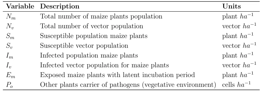
Table 1: Variables and their description
Variable Description Units
Nm Total number of maize plants population plant ha−1
Nv Total number of vector population vectorha−1
Sm Susceptible population maize plants plantha−1
Sv Susceptible vector population vectorha−1
Im Infected population maize plants plantha−1
Iv Infected vector population for maize plants vectorha−1
Em Exposed maize plants with latent incubation period plantha−1
Po Other plants carrier of pathogens (vegetative environment) cells ha−1
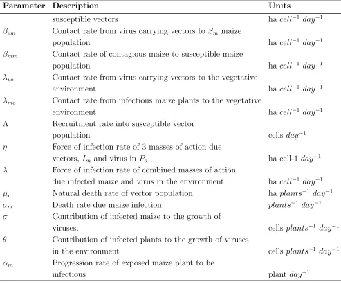
Table 2: Parameters and their description
Parameter Description Units
βmv Contact rate from infected maize to susceptible vector
population hacell−1 day−1
µo Natural death rate of vector within environment haplants−1 day−1
βo Contact rate of other plants (not maize) carrying
pathogen with maize hacell−1 day−1
βov Contact rate of virus in the environment to the
Table 2 –Continued from previous page
Parameter Description Units
susceptible vectors hacell−1 day−1
βvm Contact rate from virus carrying vectors to Sm maize
population hacell−1 day−1
βmm Contact rate of contagious maize to susceptible maize
population hacell−1 day−1
λvo Contact rate from virus carrying vectors to the vegetative
environment hacell−1 day−1
λmo Contact rate from infectious maize plants to the vegetative
environment hacell−1 day−1
Λ Recruitment rate into susceptible vector
population cells day−1
η Force of infection rate of 3 masses of action due
vectors,Im and virus in Po ha cell-1 day−1
λ Force of infection rate of combined masses of action
due infected maize and virus in the environment. hacell−1 day−1
µv Natural death rate of vector population haplants−1 day−1
σm Death rate due maize infection plants−1 day−1
σ Contribution of infected maize to the growth of
viruses. cells plants−1 day−1
θ Contribution of infected plants to the growth of viruses
in the environment cells plants−1 day−1
αm Progression rate of exposed maize plant to be
2.2. Model flow chart. Using assumptions of the model and defined
variables/parameters, the dynamics of maize lethal necrosis disease (MLND) in maize population can be shown as the flow chart in Figure 1 depicts.
Figure 1. Schematic of MLND with susceptible maize plants population
which interacts with forces of infection from viruses in the environment (Po),
infected maize (Im) and infected vector (Iv) populations. Epidemic starts from
susceptible maize (Sm) and moves to exposed class (Em) and infected class (Im)
respectively.
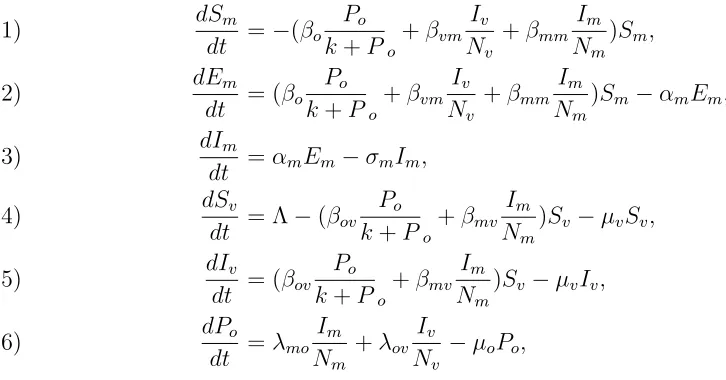
2.3. Equations of the model. Considering the compartmental diagram as described by Figure 1, we formulate basic mathematical model which shows transmission dynamics for MLND using the following differential equations:
dSm
dt =−(βo Po
k+Po
+βvm
Iv
Nv
+βmm
Im
Nm
)Sm,
(1)
dEm
dt = (βo Po
k+Po
+βvm
Iv
Nv
+βmm
Im
Nm
)Sm−αmEm,
(2)
dIm
dt =αmEm−σmIm,
(3)
dSv
dt = Λ−(βov Po
k+Po
+βmv
Im
Nm
)Sv −µvSv,
(4)
dIv
dt = (βov Po
k+Po
+βmv
Im
Nm
)Sv −µvIv,
(5)
dPo
dt =λmo Im
Nm
+λov
Iv
Nv
−µoPo,
(6)
with initial conditions:
Note that the total number of maize plants population is given by
(7) Nm =Sm+Em+Im,
while the total number of vector population is given by
(8) Nv =Sv +Iv.
2.4. Basic properties of the model. In order to see if the model is mathematically and epidemiologically well posed to study the MLND dynamics, we considered two basic proper-ties of the model. We used Box invariant of Metzler Matrix to show the existence of invariant region [6, 7] and basic standard method to prove the positivity of solutions.
2.4.1. Invariant region. We proof the invariant region as follows: The system of the model
(1) can be written as
dX
dt =A(X)X+F withX=(Sm, Em, Im, Sv, Iv, Po)
T and the constant termF = (0,0,0, λ,0,0)T.
That is
A(X) =
−Fm 0 0 0 0 0
Fm −αm 0 0 0 0
0 αm −σm 0 0 0
0 0 0 −Fv−µv 0 0
0 0 0 Fv −µv 0
0 0 λmo
Nm 0
λov
Nm −µo
and
Fm =(βo
Po
k+Po
+βvm
Iv
Nv
+βmm
Im
Nm
),
Fv =(βov
Po
k+Po
+βmv
Im
Nm
).
A(X) is a Metzler Matrix ∀ X∈ R6+ which all off diagonal terms are non negative and
F ≥0.The system dXm
dt =A(X)X +F is positive invariant in R
6
+. We can conclude that the
feasible region Ω is a set of Ω=(Sm, Em, Im, Sv, Iv, Po)∈R6+ with initial data
Sm > 0,Em ≥ 0,Im ≥ 0,Sv ≥ 0,Iv ≥ 0,Po ≥ 0. Hence, the solution stays in the region if it
started in the region.
Similarly, letting the initial data be {Sm(0), Em(0), Im(0), Iv(0), Po(0)} ∈Ω and using
stan-dard method, the solution set {Sm, Em, Im, Sv, Iv, Po}of the model system (1) was shown to
be non negative∀t ≥0. It was therefore concluded that the solution set Ω={Sm, Em, Im, Sv, Iv, Po}
of the model system (1) is non-negative for all t >0 and so it is sufficient to study the
3. Model Analysis
3.1. Existence of disease free equilibrium point. The disease free equilibrium (DFE) point of the model system (1) is given by
(9) E0 = (Sm, Em, Im, Sv, Iv, Po) = (Nm,0,0,
Λ
µv
,0,0).
When there is no disease, there will be susceptible maize population plants, Nm. On the
other hand in the susceptible vector population there will be new reproduction of vectors Λ
and dyingµv,
where Nm is the constant with adoption value of 44,000 [8] maize population in one hector.
3.2. The basic reproduction number Ro. Analysis of the equilibrium point, is carried
out by considering spectral radius of the matrix F V−1 called threshold quantity. The basic
reproduction number is the measure of secondary contagious number as a results of one contagious maize plant in the susceptible maize population.
With the help of Next Generation Matrix, the approach adopted, we determine the basic reproduction number [9]. We consider the population distinguished by six different classes
which are Sm, Em, Im, Sv, Iv and Po.
Firstly we arrange the system to get group of infectious classes only that is (Em, Im, Iv, Po).
Once again we assume fj(x) be the rate of introduction of new infectious (transmission) in
compartment i,vj+(x) be the transmission after new infectious (transition rate by all other
means) and vj−(x) rate of transfer of individual out of compartment j.
The disease transmission model comprised of the system of equations
Xj0 =fj(x)−vj(x),
where
vj(x) =v+j (x)−v
−
j (x).
To obtain the matrices F and V of dimension ’n’by’n’ we differentiate vectors fj(x) and
vj(x) respectively.
F = (∂fj(x)
∂xi
),
V = (∂vj(x)
∂xi
),
with
1≤j, i≤n,
(fj(xo)) = Fm 0 Fv 0
and, (vj(xo)) =
αmEm
−αmEm+σmIm
µvSv
λmoNImm +λovNIvv −µoPo ,
Fm = (βokP+oP o+βvmNIvv +βmmNImm)Sm,
Fv = (βovkP+oP o+βmvNImm)Sv.
Differentiate (Fm, Fv,0,0)T with respect to (Em, Im, Iv, Po)T and obtain
F =
0 βmmNSmm βvmNSmv βo(kkS+Pm)2
0 0 0 0
0 βmvNSv
m 0 βov
kSv
(k+P)2
0 0 0 0
.
At disease free Sm = Nm which is the number of maize grains sowed and germinated in a
maize plant, and Sv = µΛv as from
dSv
dt = Λ−(βov Po
k+P o+βmv Im
Nm)Sv−µvSv.
Hence matrix F reduces to
F =
0 βmm βvmNm
Nv
βoNm k
0 0 0 0
0 βmvNmΛµv 0 βovµvΛK
0 0 0 0
.
Again differentiate vj(xo) =
αmEm
−αmEm+σmIm
µvSv
λmoNImm +λovNIvv −µoPo
with respect to (Em, Im, Iv, Po)T to obtain matrix V.
Hence, V =
αm 0 0 0
−αm σm 0 0
0 0 µv 0
0 −λmo
Nm − λov Nv µ0
.
We find the inverse of V i.e
V−1 =
1
αm 0 0 0
1 αm
1
σm 0 0
0 0 µ1
v 0
λmo Nmσmµo
λmo Nmσmµo
λvo Nvµvµ0
And multiplying matrix F and V−1 we obtain
F V−1 =
βmm σm +
βoλmo kσmµo
βmm σm +
βoλmo kσmµo
βvmNm Nvµv +
λvoβoNm kNvµvµo
βoNm kµo
0 0 0 0
βmvΛ Nmσmµv +
λmoβovΛ kNmσmµvµo
βmvΛ Nmσmµv +
λmoβovΛ kNmσmµvµo
λvoβovΛ kNvµ2vµo
βovΛ kµvµo
0 0 0 0
.
According to [10] the matrix can be reduced into 2 by 2 matrix. [11] The dominant
eigen-value of this matrix is Ro, which can be obtained from the trace and determinant of that
matrix as
K =
βmm σm +
βoλmo kσmµo
βvmNm Nvµv +
βoNmλvo kNvµvµo
βmvΛ Nmµvσm +
βovΛλmo kµvNmσmµo
βovΛλvo kµoNvµv2
.
T race(K) = βmm
σm
+ βoλmo
kσmµo
+ λvoβovΛ
kNvµ2vµo
or in a simple form:
T race(K) = Nmµ
2
v(kβmmµo+βoλmo) +λvoβovΛ
kNvµ2vµo
.
Det(K) = − Λ (kβmvβvmµo−βmmβovλvo +βmvβoλvo +βovβvmλmo)
kµoNvµv2σm
.
But according to [10] we have this formula for
Ro =ρ(K) =
1 2
T race(K) +pT race(K)2−4det(K).
We substitute trace and determinant in the formula above and obtain a condensed form as shown below.
Ro =ρ(K) =
1 2
βmm
σm
+ βoλmo
kσmµo
+ Λ
Nv
λvoβov
kµ2 vµo
(10) +1 2
s
βmm
σm
+ βoλmo
kσmµo
+ Λ
Nv
λvoβov
kµ2
vµo
2
+ 4Λ
Nv
kβmvβvmµo−βmmβovλvo+βmvβoλvo+βovβvmλmo
kµoµv2σm
.
3.3. Endemic equilibrium point. Endemic equilibrium point of the model system (1)
E∗ is a steady state solution where by the disease persists in the population or an
equi-librium comprised of diseased sub-populations i.e. Em 6= 0, Im = 0,6 Iv 6= 0 and Po 6= 0.
By equating all expressions for the equations in the model system (1) to zero and let E∗
=(Sm∗, Em∗, Im∗, Sv∗, Iv∗, Po∗) we compute the system and arrive to the cubic polynomial
equa-tion as follows.
(11) P(I∗) =AI∗3+BI∗2−DI∗−C
A=βmmµ2vµoNvλmo(αm+σm),
B = (αm+σm)βoµ2vµoNv2Nmλmo+βmvµvµoNmλmoΛ(αm+σm) +βmmµ2vµ 2 oN
2
vNmk(αm+σm)
+βmmµoµvNmNvλovΛ(αm+σm)>−βmmµv2µoNmNvλmoαm−σmµ2vµoNv2αmλov,
D=−βoµoµvNm2NvλovΛ(αm+σm) +βmvµvµ2oN 2
mNvΛαmk(αm+σm)
−βmvµoNm2Λ 2
αmk(αm+σm)−βoµ2vµoNm2N 2
vλmoαm
−βmmµvµoNm2NvΛαm−βmmµ2vµ 2 oN
2 mN
2 vkαm
−µvµoNm2NvλmoΛσmαm−µ2vµ 2 oN
2 mN
2
vkσmαm,
C =−βoµvµoNm3NvλovΛαm−βmvµvµo2Nm3Nvλovkαm−βmvµoNm3NvλovΛ2αm.
The obtained polynomial function with cubic degree indicates the existence of endemic equi-librium points. Using Maple 18 (32 bit) we solve the polynomial equation to obtain three distinct roots of which one is real and the other two are complex.
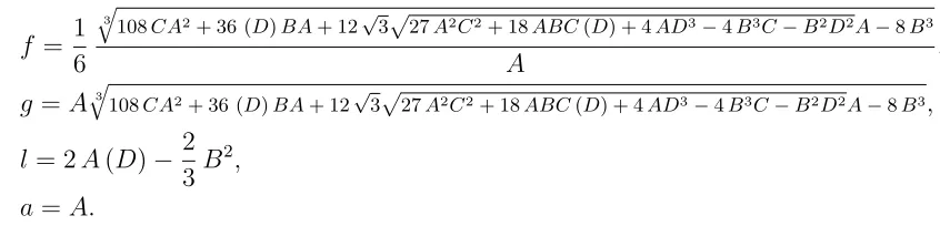
We rely on the real root and define an equilibrium point which is comprised of epidemic populations and given by the endemic equilibrium point as
(12) (Ee) =
Sm∗ Em∗ Im∗ Sv∗ Iv∗ Po∗
= Λ1 Λ2 Λ3 Λ4 Λ5 Λ6 , where
Λ1 =Nm−(
αm+σm
αm
)af
2−6ag−6a2f l
6a2f ,
Λ2 =
σm
αm
af2−6ag−6a2f l
6a2f
,
Λ3 =
Af2−6ag−6a2f l
6a2f ,
Λ4 =
Λ
βovPo k+Po +
βmvIm∗ Nm +µv
,
Λ5 =
βovPo k+Po +
βmvIm∗ Nm +µv
2
Λµv
,
Λ6 =
λmoIm∗
µoNm
+ λovΛ
and
f = 1 6
3
q
108CA2+ 36 (D)BA+ 12√3p
27A2C2+ 18ABC(D) + 4AD3−4B3C−B2D2A−8B3
A ,
g =Aq3
108CA2+ 36 (D)BA+ 12√3p27A2C2+ 18ABC(D) + 4AD3−4B3C−B2D2A−8B3, l = 2A(D)− 2
3B
2
,
a=A.
3.4. Sensitivity analysis. Sensitivity analysis can applied to test the ability of the model in relation to prediction of model parameters[11]. In this section we use sensitivity analysis
to determine the impact of parameters on Ro. In order to determine an excellent way that
can reduce maize death and morbidity due MLND, it is crucially important to understand the proportional importance of factors that are liable for the transmission and prevalence of the infection.
Table 3 shows the parameter values of maize disease model. The parameters are taken from the previous studies that correspond to this study, existing information and through approximation.
To perform sensitivity analysis of Ro we need to first determine sensitivity indices’s for each
of parameters.
We define sensitivity indices’s as partial derivative of Ro with respect to a given parameter
as multiplied by the ratio of given parameter to the basic reproduction number Ro.
Mathematically, this definition is given by:
(13) rRo
mi = (
∂Ro
∂mi
)× mi
Ro
.
The approach used in equation (13) above is called normalized forward sensitivity indices of
Ro with respect to parametersmi, wheremi is any parameter from Ro.
3.5. Parameters estimation and adoption. In this subsection, we will review some jour-nals to get proper parameters and where necessary approach of estimation will be used. The primary infection rate of other plants population rather than maize can be greater or equivalent to 0.02 i.e 0.04,0.06,0.08... [12]
Transmission of Maize Chlorotic Mottle Virus by Chrysomelid Beetles and its cleoptera species of 8 classes was estimated [13]. From acquisition to inoculation is 8 days. The rates of these different classes were 0.390.0.905,0.052,0.024,0.170,0.139,0.156 and 0.Finding the av-erage we obtain 0.2295 and again divide by 8 days and results to our one of transmission
rate βmm 0.0286875.
Leafhopper transmission rate of ACMV 0.020(standard) 0.005 to 0.100 (range) (diseasedplant)−1day−1
and transmission rate of EACMV 0.030 (standard) 0.01 to 0140 (range) (diseasedplant)−1day−1
(0.008 0.04), the insects have crucial role in disease transmission and as the matter of fact leafhoppers are responsible by settling on the crops[15].Therefore, from this description we can estimate some of our model parameters between such interval as from 0.005 to 0.100 as we can see in the Table 3.
Vector carrying capacity per plant k = 50,Vector birth rate 0.11.2, Vector death rate
0.05,Disease-induced mortality rate (roguing) 0.02 [16].
Other plants transmission and roguing rate are 0.0064 and 0.00033 respectively[17]. Maize
recruitment rate 276.8212,contact rate of maize plants with pathogen β 0.0024,net decay
rate of pathogens 0.85,contributions of I(t) to the growth of pathogen 0.0018, natural death
rate of Sm 0.00033113 ,death rate of Im due to foliage disease 0.00099338,total population
of 44,000 maize plants per ha and maturity of maize plants from day one the harvest day is 151 days[8].It can also be noted that 90 days are also applicable for short season.
Table 3 summaries the estimated and collected data as
follows:-Table 3: Parameters values for MLND model.
Parameters Values Units Reference/Source
k 10 ha plant−1 estimated
βo 0.06 ha cells−1day−1 [12]
βov 0.06 ha cells−1day−1 [12]
Nv 2,800 ha ha−1 estimated
βmm 0.286875 ha cells−1day−1 [13]
λvo 0.07486 ha cells−1day−1 estimated
λmo 0.010 ha cells−1day−1 estimated
Λ 0.95 ha vectors−1day−1 estimated
µv 0.05 ha vectors−1day−1 [16]
σm 0.02 ha plants−1day−1 [16]
µo 0.0005 ha pathogens−1day−1 estimated
βmv 0.0024 ha cells−1day−1 [14]
βvm 0.024 ha cells−1day−1 [14]
αm 0.020 ha cells−1day−1 [15]
Nm 44,000 ha ha−1 [8]
σ 0.0018 ha cells−1day−1 [8]
The numerical value of Ro referred from equation (10) is given by Ro = 7.54 .
Table 4: Sensitivity indices determined based on param-eter values.
Parameters Values Sensitivity indices
k 10 -0.8122148385
βo 0.06 0.7996312039
βov 0.06 0.01258363435
Nv 2,800 -0.01293729282
βmm 0.286875 0.1869621680
λvo 0.07486 0.01246795692
λmo 0.010 0.7997468812
Λ 0.95 0.01293729256
µv 0.05 -0.02587458659
σm 0.02 -0.9870627077
µo 0.0005 -0.8122148376
βmv 0.0024 0.00035365821
βvm 0.024 0.00046933564
From Table 4 we discover that the most positively sensitive parameter is the rate of
interac-tion between contagious maize sub-populainterac-tion and environment λmo. In fact any movement
of pathogens either from infected/environment to environment/infected cause much damage maize population. The parameter adequate or close to the most positively sensitive is the
interaction between virus in the environment to susceptible maize sub-populationβo, to this
juncture there is no doubt that environment plays crucial role in transmitting MLND. There is also positive moderate transmission of disease through maize to maize contact which is
due to adequate contact rate of infected to susceptible maize sub-populations βmm, this is
probably because there is a bit distance apart between one line and the other. The less
sensitive positive parameters are Λ,λvo, βov, βmv and βvm.
It can also be noted that, the most negatively sensitive parameter is the disease induced
death rate σm and the negatively adequate rates are natural mortality rate µo and the
car-rying capacity of virus in the environment k, while the less negatively sensitive parameters
are mortality natural death of vector µv and total number of vectors Nv.
It is important to note that, the increase of any of positively sensitive parameter increases
Ro and decreasing any of these decreases Ro as well, while decreasing any of the negatively
sensitive parameter increases Ro and increasing any of them decreasesRo too.
for control strategies.
3.6. Simulation of the basic model. In this subsection we will deal with basic model simulations. We will see the behavior of MLND dynamics when endemic exists and show how maize populations react towards vectors population and environment as well. Further-more, we will show the effects of most sensitive and adequate parameters in regards to basic reproduction number.
All simulations are carried out using MATLAB R2013a and HP Windows 7 Professional/ Intel(R) Core (TM)i3-4005U CPU @1.70GHz 1.70GHz Computer machine.
3.7. Dynamics of populations simulation. We simulate maize,vectors and viruses in the environment populations before looking into behavior and formation MLND based on 151 days the maize duration from planting to the harvesting day.
From Figures 2 and 3: We observe six different lines as an indication of various popula-tions. The green, cyan, black are three different lines which compose maize populations of at risk (susceptible), exposed and infested population respectively. The susceptible maize population decelerates exponentially to acquire endemic equilibrium level as they die due MLND which is the effects of maize to maize infection, virus in the environment and infected vector population. The exposed maize population assumes parabolic curve as it increases exponentially to a certain maximum point before exponential deceleration to the a certain endemic level. This behavior explain the incubation period that some resistant maize plants takes after exposed as it keeps increasing before turn slowly into infection class.
The red line is the susceptible vectors and the blue line is infested vectors. The susceptible vectors decrease exponentially due to natural death and acquisition of infestation from se-verely infested maize, vectors and environment and finally acquire the endemic equilibrium level. The infested vectors forms parabolic curve as they do raise and drop exponentially to the endemicity level. The raising to the maximum point implies decrease of susceptible vectors add members to the infestation vectors and some might come from environment and infected maize. On the other hand the exponential dropping indicates no more susceptible vectors which means recruitment rate is much less as compared to both dying and infection rate.
0 20 40 60 80 100 120 140 160 0
0.5 1 1.5 2 2.5 3 3.5
4x 10
4
Time[days]
Populations
MATHEMATICAL MODEL SIMULATION
Sm= Susceptible maize
Im= Infected maize
Em= Exposed maize
Sv= Susceptible vectors
Iv= Infected vectors
Po= Virus in evironmen
0 20 40 60 80 100 120 140 160
49 50 51 52 53 54 55
Time[days]
Virus in the environment/ha
VIRUSES IN THE ENVIRONMENT VS TIME(DAYS)
Figure 2. with sub-figure 2a and 2b respectively
This Figure is showing fully simulated model and partly in the environment with the MLND dynamics of sub-populations/ha
3.8. The effects of parameters on basic reproduction number. We refer Figures 4, 5 and 6 to illustrates the effect of the most sensitive and moderate positive indexes as well as the most sensitive and moderate negative indexes parameters on the basic reproduction number.
In Sub-figures 4a and 5b we note λmo is the most sensitive positive parameter, that the
increase of this transmission rate result to the quick increase of the basic reproduction number.It imply that the interaction of infested sub-population(maize/pathogens) might have significant effects on maize population. Similarly, the maize death rate due to disease
σm is the most sensitive negative parameter, that any reduction from it (stop dying of maize)
make basic reproduction number experience significant exponential retardation. In other words, susceptible maize population will always remain constant if there is no infestation. From Sub-figures 4b and 5a we observe significant steep slope increase of basic reproduction
number as the increase of each of these parameters (βo and βmm as proceeds additional
positive increments. The reason behind these rapid positive increments might be the main causative of MLND arises from the contact rate from infected maize to other vegetative plants and interaction of infested to susceptible maize rates.
Sub-figures 6a and 6b illustrates the principal effects of natural death rate of vectors in the environment and the carrying capacity. Both of these moderate rate reduces exponentially to zero as basic reproduction number do and to the contrary is also true. This behavior gives an indication that killing of vectors both in the environment and its population will have significant effects on MLND reduction if not eradication of the whole epidemic since any mortality rate does not favor pathogens but maize population.
0 20 40 60 80 100 120 140 160 0 0.5 1 1.5 2 2.5 3 3.5
4x 10
4
Time[days]
Maize populations/ha
MAIZE POPULATION VS TIME (DAYS)
Sm= Susceptible maize
Im= Infected maize
Em= Exposed maize
0 20 40 60 80 100 120 140 160
0 500 1000 1500 2000 2500 Time[days] Vectors populations/ha
VECTORS POPULATION VS TIME (DAYS)
Sv= Susceptible vectors
Iv= Infected vectors
Figure 3. with sub-figure 3a,3b respectively
This figure depicts the MLND dynamics partly in maize and partly in vector model sub-populations/ha
0 0.001 0.002 0.003 0.004 0.005 0.006 0.007 0.008 0.009 0.01
4 6 8 10 12 14 16 18 20 22 24
Maize to environment contact rate(λmo)
Basic reproductive number (R
0
)
0 0.005 0.01 0.015 0.02 0.025 0.03
18 18.5 19 19.5 20 20.5 21 21.5 22 22.5
Maize to maize contact rate(βmm)
Basic reproductive number (R
0
)
Figure 4. Sub-figure 4a,4b respectively
This figure illustrates the effect ofλmo and βmm on the basic reproduction number
0 0.01 0.02 0.03 0.04 0.05 0.06
4 6 8 10 12 14 16 18 20 22 24
Environment to maize contact rate(βo)
Basic reproductive number (R
0
)
0 1 2 3 4 5 6
x 10−4
0 100 200 300 400 500 600 700 800 900 1000
Natural death rate of vector in the environment(µo)
Basic reproductive number (R
0
)
Figure 5. Sub-figure 5a,5b respectively
And this show the effects of βo and µo on the basic reproduction numberRo
0 1 2 3 4 5 6 7 8 9 10
0 100 200 300 400 500 600 700 800 900 1000 Carrying capaity(k)
Basic reproductive number (R
0
)
0 0.002 0.004 0.006 0.008 0.01 0.012 0.014 0.016 0.018 0.02
6 8 10 12 14 16 18 20 22 24
Maize induced death rate(σm)
Basic reproductive number (R
0
)
Figure 6. Sub-figure 6a,6b
The last Figure which illustrates the effect of carrying capacity and maize disease induced
The disease free equilibrium (DF E) was determined which showed that in the absence of disease only constant susceptible maize population exists with recruitment and naturally dying of vectors. Other analytical results shows that the system has unique endemic
equilib-rium point (EE) as it can be referenced from equation (12). The basic reproduction number
Ro determined was 7.54 which show that disease is endemic, cementing the point that the
system has unique endemic equilibrium point.From the literature review data were collected and summarized in Table 3 which are important for model simulations, sensitivity analysis. Table 4 summaries the work of sensitivity analysis with indexes that are most, adequate and least positively and negatively sensitive crucially for transmission of MLND.
Finally, numerical simulation is done to illustrate the dynamics behavior of MLND in maize
population and how some most sensitive parameters affects Ro. It also suggest that viruses
in the environment, infected maize and vector populations plays significance role in bringing in infection force which contribute largely to the dynamics of MLND in the maize popula-tion. This situation can be seen from Figures 2 and 3 where susceptible maize and vectors decreases exponentially while others assumes exponential curves to a certain point in time by increasing before they decline and find convergence point of a certain unique endemic
equilibrium points. Another evidence is taken from Figures 4, 5 and 6 where by Ro
in-creases/decreases either with steep slopes or exponential curves as we vary by the most or adequate positively/negatively sensitive parameters. Lastly, the closer observation on basic
reproduction number, sensitivity analysis and simulation indicates that λmo, βo and βmm
parameters are main agents of transmission and persistence of epidemic and also very im-portant in finding how and where to implement the control policies for the elimination of MLND. The numerical solutions predict the danger of losing almost all crops if control mea-sures are not put into consideration since without intervention the population will vary for sometimes and ultimately they all keep approaching to endemic points and after a number of days all susceptible maize will be infected and die of disease.
In general, we formulated and analyzed a mathematical model for dynamics of MLND for a single season maize populations. This model is quite simple to start with in studying and analyzing the dynamics of maize lethal necrosis disease in regards to maize populations as there are a lot of complications if we consider in depth the epidemiological process of MLND. Therefore study will add value to body of knowledge, policy makers and act as a bridge for researchers who would like to study the dynamics of MLND mathematically.
Acknowledgments
sincere gratitude to the Higher Education Students Loan Board (HESLB) for funding this program.
References
[1] I. Adams, D. Miano, Z. Kinyua, A. Wangai, E. Kimani, N. Phiri, R. Reeder, V. Harju,
R. Glover, U. Hany, et al., “Use of next-generation sequencing for the identification
and characterization of maize chlorotic mottle virus and sugarcane mosaic virus causing
maize lethal necrosis in kenya,”Plant Pathology, vol. 62, no. 4, pp. 741–749, 2013.
[2] A. Wangai, M. Redinbaugh, Z. Kinyua, D. Miano, P. Leley, M. Kasina, G. Mahuku, K. Scheets, and D. Jeffers, “First report of maize chlorotic mottle virus and maize lethal
necrosis in kenya,” Journal of Virological Methods, vol. 240, pp. 49–53, 2017.
[3] M. Gowda, B. Das, D. Makumbi, R. Babu, K. Semagn, G. Mahuku, M. S. Olsen, J. M. Bright, Y. Beyene, and B. M. Prasanna, “Genome-wide association and genomic prediction of resistance to maize lethal necrosis disease in tropical maize germplasm,”
Theoretical and Applied Genetics, vol. 128, no. 10, pp. 1957–1968, 2015.
[4] F. H. Kiruwa, T. Feyissa, and P. A. Ndakidemi, “Insights of maize lethal necrotic disease:
A major constraint to maize production in east africa,”African Journal of Microbiology
Research, vol. 10, no. 9, pp. 271–279, 2016.
[5] D. W. Miano, “Maize lethal necrosis disease: A real threat to food security in the eastern and central africa region,” 2014.
[6] J. Kahuru, L. Luboobi, and Y. Nkansah-Gyekye, “Stability analysis of the dynamics of
tungiasis transmission in endemic areas,” Asian Journal of Mathematics and
Applica-tions, vol. 2017, pp. 1–24, 2017.
[7] A. Abate and A. Tiwari, “The concept of box invariance for special classes of dynamical
systems,” inProceedings of the 45th IEEE Conference on Decision and Control, Citeseer,
2007.
[8] O. C. Collins and K. J. Duffy, “Optimal control of maize foliar diseases using the plants
population dynamics,”Acta Agriculturae Scandinavica, Section BSoil & Plant Science,
vol. 66, no. 1, pp. 20–26, 2016.
[9] R. C. Ngeleja, L. S. Luboobi, and Y. Nkansah-Gyekye, “Modelling the dynamics of
bubonic plague with yersinia pestis in the environment,” Communications in
[10] O. Diekmann, J. Heesterbeek, and M. Roberts, “The construction of next-generation
matrices for compartmental epidemic models,” Journal of the Royal Society Interface,
pp. 873–885, 2009.
[11] S. Edward, D. Kuznetsov, and S. Mirau, “Modeling and stability analysis for a varicella
zoster virus model with vaccination,” Applied and Computational Mathematics, vol. 3,
no. 4, pp. 150–162, 2014.
[12] L. V. Madden and F. Van Den Bosch, “A population-dynamics approach to assess the threat of plant pathogens as biological weapons against annual crops using a coupled differential-equation model, we show the conditions necessary for long-term persistence of a plant disease after a pathogenic microorganism is introduced into a susceptible
annual crop,” BioScience, vol. 52, no. 1, pp. 65–74, 2002.
[13] L. Nault, W. Styer, M. Coffey, D. Gordon, L. Negi, C. Niblett, et al., “Transmission
of maize chlorotic mottle virus by chrysomelid beetles,” Phytopathology, vol. 68, no. 7,
pp. 1071–1074, 1978.
[14] X.-S. Zhang, J. Holt, and J. Colvin, “Synergism between plant viruses: a mathematical
analysis of the epidemiological implications,” Plant Pathology, vol. 50, no. 6, pp. 732–
746, 2001.
[15] M. Zhao, H. Ho, Y. Wu, Y. He, and M. Li, “Western flower thrips (frankliniella
occi-dentalis) transmits maize chlorotic mottle virus,” Journal of Phytopathology, vol. 162,
no. 7-8, pp. 532–536, 2014.
[16] M. Jeger, Z. Chen, G. Powell, S. Hodge, and F. Van den Bosch, “Interactions in a host plant-virus–vector–parasitoid system: Modelling the consequences for virus transmission
and disease dynamics,” Virus research, vol. 159, no. 2, pp. 183–193, 2011.
[17] Z. Zhonghua and S. Yaohong, “Stability and sensitivity analysis of a plant disease model
with continuous cultural control strategy,” Journal of Applied Mathematics, vol. 2014,
pp. 1–15, 2014.
1
Department of Applied Mathematics and Computational Science, Nelson Mandela African
Institution of Science and Technology,P.O.Box 447, Arusha, Tanzania
2
Institute of Mathematical Sciences, Strathmore University, P.O. Box 59857 - 00200, Nairobi, Kenya
3
Department of Secondary Education,Moshi Municipal Council,P.O.Box 318, Moshi,Tanzania