R E S E A R C H
Open Access
Dynamic study of a predator-prey model
with Allee effect and Holling type-I functional
response
Yong Ye
1, Hua Liu
1*, Yumei Wei
2, Kai Zhang
1, Ming Ma
1and Jianhua Ye
1*Correspondence:
1School of Mathematics and
Computer Science, Northwest Minzu University, Lanzhou, People’s Republic of China
Full list of author information is available at the end of the article
Abstract
In this paper, a prey-predator model with Allee effect and Holling type-I functional response is established, and its dynamical behaviors are studied in detail. The existence, boundedness and stability of the model are qualitatively discussed. Hopf bifurcation analysis is also taken into account. We further illustrate our theoretical analysis by means of numerical simulation. Using computer simulation, we found the position of each equilibrium point in the phase diagram that we drew. We found the threshold for undergoing a Hopf bifurcation in the bifurcation diagram. One of the interesting questions is which model with strong Allee effect is a bistable system.
Keywords: Allee effect; Prey-predator; Bistable; Stability; Hopf bifurcation
1 Introduction
Today, in order to comprehend the long-term behavior of a population, many researchers conduct extensive research on the dynamics of interacting prey-predator models. Vari-ous nonlinear ODE models are studied, and the interaction between predator and prey is analyzed [1–24]. The classic predator-prey model is the Lotka–Volterra model, which was independently proposed by Lotka in the United States in 1925 and Volterra in Italy in 1926. However, there are some specific classes among them, called the Gause type models [1,2]. The research of predator-prey model and infectious disease model has always been a hot topic in biomathematics [1–9,11–31]. In 1931, Allee discovered that the living state of the cluster is conducive to the growth of the population, but the density is too high and will inhibit the growth of the population and even become extinct due to resource com-petition. For each population, there must be an independent optimal density for growth and reproduction, the mechanism is called the Allee effect. There are also lots of people doing research on the predator-prey model with Allee effect in prey growth [3,8,9,12,
14,22,24].
We consider the predator-prey model with Allee effect and Holling type-I functional response in predator growth [3] as follows:
dN
dT =Ng(N) –p(N)P, dP
dT =cp(N) –q(P)P,
(1)
whereg(N) =r(1 – NK)(N–L) andp(N) =aN, and the initial condition isN(0),P(0) > 0. Nis the prey population andPis the predator population,q(P) is the average loss rate of predators,cis the conversion efficiency from prey to predator,Kis the carrying capacity, g(N) is the per capita prey growth rate,ris the intrinsic growth rate of prey,Lis the Allee effect threshold,p(N) is the prey dependent functional response, andais the prey capture rate by their predators. So we get
dN dT =Nr
1 –N
K
(N–L) –aNP,
dP
dT =c(aN)P–mP,
(2)
whereaandmare all positive parameters.mis the intrinsic death rate of the predators.
2 Strong Allee effect
In order to reduce the number of parameters in the latter calculation, we can make model (2) dimensionless as follows:
dx
dt =x(1 –x)(x–β) –αxy, dy
dt=γxy–δy,
(3)
wherex=NK,y=P,t=KrT,α=Kra,β=KL,γ =car andδ=Krm. It is easy to see 0≤x≤1. The threshold of the Allee type isβand satisfies the conditions 0 <β< 1 for a strong Allee effect [3].
3 Equilibria and existence
In order to find the equilibrium point of model (3), we consider the prey and predator nullcline of this model (3), to get
x(1 –x)(x–β) –αxy= 0,
γxy–δy= 0,
we easily see that model (3) exhibits four equilibrium pointsEs0= (0, 0),Es1= (β, 0),Es2=
(1, 0),Es∗= (x∗,y∗). Herex∗=γδ,y∗=
(1–γδ)(δγ–β)
α . For a positive equilibrium point, we have β<γδ < 1.
4 Boundedness of the model
Theorem 1 All the solutions of model which start in R2
+are uniformly bounded.
Proof A function is defined by us that isχ=x+γ–αδ+ηy. Therefore, the time derivative of the above equation along the solution of model (3) is
dχ dt =
dx dt +
α γ –δ+η
dy dt
= –x3+ (1 +β)x2–βx–αxy+ α
Now for eachη> 0 and 0≤x≤1, we have
In this section, we will analyze the local stability of model (3).
Theorem 2
(1) Es0is locally asymptotically stable.
(2) Ifγ<βδ,thenEs1is the saddle point,otherwise it is the unstable node.
(3) Whenγ <δ,Es2is locally asymptotically stable and is a saddle point otherwise. (4) The positive equilibriumEs∗is locally stable whenβ<2δγ–γ and is unstable node
otherwise.
Proof It can be concluded by calculating the Jacobian matrix of model (3) atEs0
Js0=
Also we can find thatEs0is locally asymptotically stable.
By evaluating the Jacobian matrix of model (3) atEs1, we find
We calculate the Jacobian matrix of model (3) atEs2; we have
Js2=
β– 1 –α 0 γ –δ
.
We find that the first eigenvalueλ1=β– 1 is negative because ofβ< 1, thenEs2is stable
ifγ <δ, andEs2is a saddle point whenγ >δ.
We calculate the Jacobian matrix of model (3) atEs∗is given by
Js∗=
(2 + 2β)x∗– 3x2∗–β–αy∗ –αx∗
γy∗ 0
.
We can easily know that the characteristic polynomial is
H(λ) =λ2–Tλ+D.
HereT= (2 + 2β)x∗– 3x2∗–β–αy∗andD= (1 –γδ)( δ γ –β)δ. Thus, we have the following conclusions.
(a) IfT< 0andβ<2δγ–γ, then the positive equilibrium is locally asymptotically stable. (b) IfT> 0andβ>2δγ–γ, then the positive equilibrium is unstable.
6 Bifurcation analysis
6.1 Hopf bifurcation
From Theorem2, model (3) undergoes a bifurcation ifβ=2δγ–γ. The purpose of this sec-tion is to prove that model (3) will produce a Hopf bifurcation ifβ=2δγ–γ.
First we chooseβas the bifurcation parameter, and then analyze the conditions under which a Hopf bifurcation occurs atEs∗= (x∗,y∗). Denote
β0=
2δ–γ γ ,
whenβ=β0, we haveT= (2 + 2β)x∗– 3x2∗–β–αy∗= 0. Thus, the Jacobian matrixJs∗has a pair of imaginary eigenvaluesλ=±i
(1 –γδ)(γδ –β0)δ. Letλ=A(β)±B(β)ibe the roots
ofλ2–Tλ+D= 0, then
A2–B2–AT+D= 0,
2AB–TB= 0
and
A=T 2,
B=
√
4D–T2
2 ,
dA dβ|β=β0=
By thePoincare–AndronovHopf bifurcation theorem, we know that model (3) under-goes a Hopf bifurcation atEs∗= (x∗,y∗) whenβ=β0. However, the directionality of the
set
Ifσ< 0, the equilibriumEs∗is destabilized through a Hopf bifurcation that is supercritical and a Hopf bifurcation that is subcritical otherwise [10].
7 Weak Allee effect
8 Equilibria and existence
In order to find the equilibrium points of model (4), which follow from
x(1 –x)(x+β) –αxy= 0,
γxy–δy= 0,
we easily see that model (4) exhibits three equilibrium points,Ew0= (0, 0),Ew2= (1, 0),
Ew∗= (x¯∗,y¯∗). Here,x¯∗=γδ,y¯∗=
(1–γδ)(γδ+β)
α . For a positive equilibrium point, we have δ γ < 1.
9 Stability analysis
In this section, we will analyze the stability of model (4).
9.1 Local stability
Theorem 3
(1) Ew0is a saddle point.
(2) Ew2is stable forγ <δ,Ew2is a saddle point forγ >δ.
(3) Positive equilibriumEw∗is locally asymptotically stable whenβ> 1 – 2x¯∗,Ew∗is an
unstable node whenβ< 1 – 2x¯∗.
Proof It can be concluded by calculating the Jacobian matrix of model (4) atEw0that
Jw0=
β 0 0 –δ
.
HenceEw0is always a saddle point.
It can be concluded by calculating the Jacobian matrix of model (4) atEw2that
Jw2=
–β– 1 –α 0 γ–δ
.
We can find that the first eigenvalueλ1= –β– 1 is negative, henceEw2is stable ifγ <δ,
andEw2is a saddle point whenγ>δ.
We calculate the Jacobian matrix of model (4) atEw∗that is given by
Jw∗=
(2 – 2β)x¯∗– 3x¯2∗+β–αy¯∗ –αx¯∗
γy¯∗ 0
.
The characteristic polynomial is
H(λ) =λ2–T¯λ+D¯,
whereT¯ = (2 – 2β)x¯∗– 3x¯2∗+β–αy¯∗andD¯ = (1 –γδ)(γδ +β)δ. Thus, we have the following conclusions.
(a) IfT¯ < 0andβ> 1 – 2x¯∗, we can find thatEw∗is locally asymptotically stable.
9.2 Global stability
Here we first prove thatEw2= (1, 0) is globally stable when (α+αγ)2–4αδ < 0.
Consider the Lyapunov function:
V(x,y) =1 2(x– 1)
2+y.
The derivative ofValong the solution of model (4) is
˙
V = (x– 1)x(1 –x)(x+β) –αxy+γxy–δy
= –x(1 –x)2(x+β) – (x– 1)αxy+γxy–δy
≤–(x– 1)αxy+γxy–δy
= –αx2y+αxy+γxy–δy
= –yαx2–αx–γx+δ
= –αy x2–
α+γ α
x+δ
α
.
Ifx2– (α+γ α )x+
δ
α> 0, thenV˙ < 0. So,= ( α+γ
α )
2–4δ α < 0.
Next, we prove thatEw∗= (x¯∗,y¯∗) is globally stable for model (4). Here, we will prove the global stability ofEw∗= (x¯∗,y¯∗) based on the fact thatEw∗= (x¯∗,y¯∗) is locally asymptotically stable by using Th. 2 in [11]. In order to use this theorem better, we can rewrite model (4) as follows:
dx
dt =xg(x) –αyp(x), dy
dt=γyp(x) –δy.
Hereg(x) = (1 –x)(x+β) andp(x) =x. Hereg(x) andp(x) satisfy the following three con-ditions:
1. g∈C([0,∞),R)∩C1((0,∞),R),g(0) = (1 – 0)(0 +β) > 0,g(1) = 0and(x– 1)g(x) < 0 forx∈[0, 1)∪(1,∞).
2. p∈C([0,∞),R)∩C1((0,∞),R),p(0) = 0andp(x) = 1 > 0for allx≥0.
3. The positive equilibrium pointEw∗= (x¯∗,y¯∗)is calculated byγp(x¯∗) –δ= 0and
¯
x∗g(x¯∗) –αy¯∗p(x¯∗) = 0,0 <x¯∗< 1,y¯∗> 0and furtherdxd( xg(x)
p(x)) = –(1 –x)(x+β) < 0, for allx¯∗<x< 1.
Here we explain the conditions. In fact, we can proceed from calculating from the local stability ofEw∗. So we can find the prey nullcliney=(1–x)(αx+β) ≡r(x) is continuous curve, we sayx=x1is a local maximum point at the points (0,βα) and (1, 0) such that 0 <x1< 1. Note thatr(x) =xgp((xx)). We can find that the condition for satisfying local asymptotic stability ofE∗is thatx=x¯∗on the right side ofx=x1and should intersect the prey nullcline, hence
0 <x¯∗<x< 1 holds. Hypothesisx1is the local maximum ofy=r(x), we know thatEw∗is locally asymptotically stable, so that dxdr(x) < 0 for 0 <x∗≤x≤1. Obviously, the above inequalities are still satisfied thatr(x) =xgp((xx)).
Theorem 4 The following condition holds:dxd(pf((xx)–)–fp((xx¯¯∗∗))) < 0for0≤x≤1and Ew∗is locally
asymptotically stable.Ew∗is globally asymptotically stable where f(x) =dxd(xg(x)) –p
(x)xg(x)
p(x) .
Proof For model (4), we can see that the definition off(x) is
f(x) = (1 –x)(x–β) +x(1 –x) –x(x+β) –x(1 –x)(x–β) x =x(1 –x) –x(x+β).
Hence we can calculate
d dx
f(x) –f(x¯∗) p(x) –p(x¯∗)
=
x(1 –x) –x(x+β) –x¯∗(1 –x¯∗) +x¯∗(x¯∗+β) x–x¯∗
=1 –β– 4x x–x¯∗ –
x–βx– 2x2– (x¯∗–βx¯∗– 2x¯2∗) (x–x¯∗)2
=x–βx– 4x
2– (x¯
∗–βx¯∗– 4xx¯∗) –x+βx+ 2x2+ (x¯
∗–βx¯∗– 2x¯2∗) (x–x¯∗)2
=–2x
2+ 4xx¯
∗– 2x¯2∗ (x–x¯∗)2 .
We find –2x2+ 4xx¯∗– 2x¯2∗< 0 for anyx> 0.
10 Hopf bifurcation
Theorem 5 By selectingβ as the bifurcation parameter,model(4)undergoes a Hopf bi-furcation that occurs at Ew∗= (x¯∗,y¯∗)ifβ= 1 – 2x¯∗.
Proof IfT¯= (2–2β)x¯∗–3x¯∗2+β–αy¯∗= 0 anddetJw∗> 0, then use the implicit function the-orem we have learned; when the stability of the equilibrium pointEw∗= (x¯∗,y¯∗) changes, Hopf bifurcation occurs, thereby generating a periodic orbit. Using these two conditions, the critical value of the Hopf bifurcation parameter is found to beβ= 1 – 2x¯∗. Obviously given the condition by [4],
(i) T¯ = (2 – 2β)x¯∗– 3x¯2∗+β–αy¯∗= 0,
(ii) detJ∗> 0, and
(iii) ddβT¯|β=β0= –
δ
γ = 0atβ=β0model (4) undergoes a Hopf bifurcation around
Ew∗= (x¯∗,y¯∗).
11 Simulations tests
In this section, we numerically simulate the above theoretical derivation by MATLAB.
11.1 Strong Allee effect
The ODE model (3) has four parameters:α,β,γ,δ. We choose the parameters
α= 0.5, β= 0.2, γ = 0.355, δ= 0.2, (5)
α= 0.5, β= 0.2, γ = 0.36, δ= 0.4, (6)
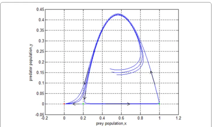
Figure 1 Es0= (0, 0) is stable,Es1= (0.2, 0) is a saddle point andEs2= (1, 0) is a saddle point
Figure 2 Es2= (1, 0) is stable
According to Fig.1, we can findEs0= (0, 0) that it is asymptotically stable. Ifγ <δthen
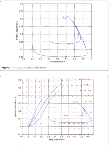
γ = 0.36 <δ= 0.4,Es2= (1, 0) is asymptotically stable as shown in Fig.2. Ifβ<2δγ–γ then 0.2 < 2∗0.2–0.290.29 ≈0.379,Es∗= (x∗,y∗) = (0.689, 0.303) is asymptotically stable as shown in Fig.3we also find the saddle pointEs1= (0.2, 0) like Fig.1. Moreover, we find that there
may be two stable equilibrium points; this is what we call a bistable system as shown in Fig.4.
Figure 3 Es∗= (x∗,y∗) = (0.689, 0.303) is stable
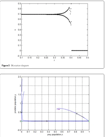
Figure 4Bistable system
11.2 Weak Allee effect
The ODE model (4) has four parameters:α,β,γ,δ. We choose the parameters
α= 0.5, β= 0.2, γ = 0.36, δ= 0.4, (8)
α= 0.5, β= 0.2, γ = 0.36, δ= 0.2, (9)
α= 0.5, β= 0.2, γ = 0.36, δ= 0.2. (10)
According to Fig.6, we can findEw0= (0, 0) to be a saddle point. Ifγ<δthenγ = 0.36 <
Figure 5Bifurcation diagram
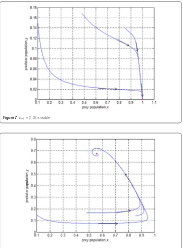
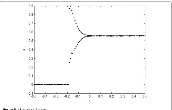
Figure 6 Ew0= (0, 0) is a saddle point,Ew2= (1, 0) is a saddle point andEw∗= (x¯∗,y¯∗) = (0.556, 0.671) is stable
1 – 2∗0.556 = –0.112,Ew∗= (x¯∗,y¯∗) = (0.556, 0.671) is asymptotically stable as shown in Fig.8.
According to Fig.9, we find that bifurcation occurs at approximatelyr= –0.112, that is, Hopf bifurcation. As we have demonstrated in the article, whenβ= –0.112, model (4) undergoes Hopf bifurcation.
12 Conclusions
Figure 7 Ew2= (1, 0) is stable
Figure 8 Ew∗= (¯x∗,¯y∗) = (0.556, 0.671) is stable
point are obtained. We analyze the Hopf bifurcation occurring atEs∗= (x∗,y∗) by choos-ingβas the bifurcation parameter, obtain the conditions for generating a Hopf bifurcation and further calculation of the Hopf bifurcation. Ifσ< 0, the equilibriumEs∗is destabilized through a Hopf bifurcation that is supercritical and the Hopf bifurcation is subcritical otherwise. The prey-predator model with weak Allee effect is also analyzed and we ob-tain stability conditions for three equilibrium points, the global stability ofEw2= (1, 0) and
equilib-Figure 9Bifurcation diagram
rium point in the phase diagram, and we draw the bifurcation diagram under the strong and weak Allee effect. It is worth noting that there are some differences between the spe-cial case of bistability and the Allee effect as regards strength and weakness. If the posi-tive equilibrium point of the model is stable, model (3) with strong Allee effect must be a bistable system. However, in the case of the weak Allee effect, the model is not necessarily a bistable system because the axial equilibrium point is unstable under certain conditions.
Funding
This work was supported by the National Natural Science Foundation of China (31560127), the Fundamental Research Funds for the Central Universities (31920180116, 31920180044, 31920170072), the Program for Yong Talent of State Ethnic Affairs Commission of China (No. [2014]121), Gansu Provincial First-class Discipline Program of Northwest Minzu University (No. 11080305) and Central Universities Fundamental Research Funds for the Graduate Students of Northwest Minzu University (Yxm2019109).
Competing interests
The authors declare that they have no competing interests.
Authors’ contributions
All authors contributed equally and significantly in this paper. All authors read and approved the final manuscript.
Author details
1School of Mathematics and Computer Science, Northwest Minzu University, Lanzhou, People’s Republic of China. 2Experimental Center, Northwest Minzu University, Lanzhou, People’s Republic of China.
Publisher’s Note
Springer Nature remains neutral with regard to jurisdictional claims in published maps and institutional affiliations.
Received: 16 December 2018 Accepted: 22 August 2019
References
1. Caughley, G., Lawton, J.H.: Plant-herbivore systems. In: May, R.M. (ed.) Theoretical Ecology, pp. 132–166. Sinauer, Sunderland (1981)
2. Freedman, H.I.: Deterministic Mathematical Models in Population Ecology. Dekker, New York (1980) 3. Banerjee, M., Takeuchi, Y.: Maturation delay for the predators can enhance stable coexistence for a class of
prey-predator models. J. Theor. Biol.412, 154–171 (2017)
4. Gupta, R.P., Chandra, P.: Bifurcation analysis of modified Leslie–Gower predator-prey model with Michaelis–Menten type prey harvesting. J. Math. Anal. Appl.398, 278–295 (2013)
6. Hu, D., Cao, H.: Stability and bifurcation analysis in a predator-prey system with Michaelis–Menten type predator harvesting. Nonlinear Anal., Real World Appl.33, 58–82 (2017)
7. Kar, T.K.: Modelling and analysis of a harvested prey-predator system incorporating a prey refuge. J. Comput. Appl. Math.185(1), 19–33 (2006)
8. Allee, W.C.: Animal Aggregations: A Study in General Sociology. University of Chicago Press, Chicago (1931) 9. Manna, D., Maiti, A., Samanta, G.P.: A Michaelis–Menten type food chain model with strong Allee effect on the prey.
Appl. Math. Comput.311, 390–409 (2017)
10. Perko, L.: Diffrential Equations and Dynamical Systems, 3rd edn. Texts in Applied Mathematics, vol. 7. Springer, New York (2001)
11. Cheng, K.S., Hsu, S.B., Lin, S.S.: Some results on global stability of a predator-prey system. J. Math. Biol.12, 115–126 (1981)
12. Cai, Y., Zhao, C., Wang, W., Wang, J.: Dynamics of a Leslie–Gower predator-prey model with additive Allee effect. Appl. Math. Model.39, 2092–2106 (2015)
13. Ghosh, J., Sahoo, B., Poria, S.: Prey-predator dynamics with prey refuge providing additional food to predator. Chaos Solitons Fractals96, 110–119 (2017)
14. Sen, M., Banerjee, M.: Rich global dynamics in a prey-predator model with Allee effect and density dependent death rate of predator. Int. J. Bifurc. Chaos25(03), 1530007 (2015)
15. Li, Y.: Hopf bifurcations in general systems of Brusselator type. Nonlinear Anal., Real World Appl.28, 32–47 (2016) 16. Yang, R., Zhang, C.: The effect of prey refuge and time delay on a diffusive predator-prey system with hyperbolic
mortality. Complexity21(S1), 446–459 (2016)
17. Ma, Z., Liu, J., Li, J.: Stability analysis for differential infectivity epidemic models. Nonlinear Anal., Real World Appl.4(5), 841–856 (2003)
18. Li, X., Jiang, W., Shi, J.: Hopf bifurcation and Turing instability in the reaction-diffusion Holling–Tanner predator-prey model. IMA J. Appl. Math.78(2), 287–306 (2013)
19. Wei, J.: Bifurcation analysis in a kind of fourth-order delay differential equation. Discrete Dyn. Nat. Soc.2009(2), 332–337 (2014)
20. Sambath, M., Balachandran, K., Suvinthra, M.: Stability and Hopf bifurcation of a diffusive predator-prey model with hyperbolic mortality. Complexity21(S1), 34–43 (2016)
21. Ma, Z., Wang, S., Wang, T., et al.: Stability analysis of prey-predator system with Holling type functional response and prey refuge. Adv. Differ. Equ.2017(1), 243 (2017)
22. Wang, J., Shi, J., Wei, J.: Predator-prey system with strong Allee effect in prey. J. Math. Biol.62(3), 291–331 (2011) 23. Rao, F., Castillo-Chavez, C., Kang, Y.: Dynamics of a diffusion reaction prey-predator model with delay in prey: effects
of delay and spatial components. J. Math. Anal. Appl.461(2), 1177–1214 (2018)
24. Feng, P., Kang, Y.: Dynamics of a modified Leslie–Gower model with double Allee effects. Nonlinear Dyn.80(1–2), 1051–1062 (2015)
25. Cai, Y., Gui, Z., Zhang, X., et al.: Bifurcations and pattern formation in a predator-prey model. Int. J. Bifurc. Chaos28(11), 1850140 (2018)
26. Zhang, H., Cai, Y., Fu, S., et al.: Impact of the fear effect in a prey-predator model incorporating a prey refuge. Appl. Math. Comput.356, 328–337 (2019)
27. Yang, B., Cai, Y., Wang, K., et al.: Global threshold dynamics of a stochastic epidemic model incorporating media coverage. Adv. Differ. Equ.2018(1), 462 (2018)
28. Cai, Y., Wang, K., Wang, W.: Global transmission dynamics of a Zika virus model. Appl. Math. Lett.92, 190–195 (2019) 29. Huang, S., Tian, Q.: Marcinkiewicz estimates for solution to fractional elliptic Laplacian equation. Comput. Math. Appl.
78(5), 1732–1738 (2019)
30. Wang, J., Cai, Y., Fu, S., et al.: The effect of the fear factor on the dynamics of a predator-prey model incorporating the prey refuge. Chaos29(8), 243 (2019)
31. Ye, Y., Liu, H., Wei, Y., et al.: Dynamic study of a predator-prey model with weak Allee effect and delay. Adv. Math. Phys.