Proceedings of the
XII Spanish Conference on Programming and Computer
Languages
(PROLE 2012)
Tabling with Support for Relational Features in a
Deductive Database
Fernando S´aenz-P´erez
16 pages
Guest Editors: Mar´ıa-del-Mar Gallardo
Managing Editors: Tiziana Margaria, Julia Padberg, Gabriele Taentzer
Tabling with Support for Relational Features in a
Deductive Database
Fernando S´aenz-P´erez1∗
Grupo de programaci´on declarativa (GPD), Dept. Ingenier´ıa del Software e Inteligencia Artificial,
Universidad Complutense de Madrid, Spain1
Abstract: Tabling has been acknowledged as a useful technique in the logic gramming arena for enhancing both performance and declarative properties of pro-grams. As well, deductive database implementations benefit from this technique for implementing query solving engines. In this paper, we show how unusual opera-tions in deductive systems can be integrated with tabling. Such operaopera-tions come from relational database systems in the form of null-related (outer) joins, duplicate support and duplicate elimination. The proposal has been implemented as a proof of concept rather than an efficient system in the Datalog Educational System (DES) using Prolog as a development language and its dynamic database.
Keywords:Tabling, Outer Joins, Duplicates, Relational databases, Deductive databases, DES
1
Introduction
Tabling is a useful implementation technique embodied in several current logic programming systems, such as B-Prolog [ZS03], Ciao [GCH+08], Mercury [SS06], XSB [SW10], and Yap Prolog [RSC05], to name just a few. This technique walks by two orthogonal axes: performance and declarative properties of programs. Tabling enhances the former because repeated computa-tions are avoided since previous results are stored and reused. The latter axis is improved because order of goals and clauses are not relevant for termination purposes. In fact, tabled computations in the context of finite predicates and bounded term depths are terminating, a property which is not ensured in top-down SLD computations.
Deductive database implementations with Datalog as query language have benefited from tabling [RU93,SSW94a,SP11] as an appropriate technique providing performance and a frame-work to implement query meaning. Terminating queries is a common requirement for database users. Also, the set oriented answer approach of a tabled system is preferred to the SLD one answer at a time.
However, “relational” database systems embed features which are not usually present alto-gether in deductive systems. These include duplicates, which were introduced to account for bags of data (multisets) instead of sets. Also, the need for representing absent or unknown in-formation delivered the introduction of null values and outer join operators ranging over such
values. Finally, aggregate functions allow to compute summarized data in terms of (multi)sets and considering null occurrences. So, these systems are not relational anymore as they depart from the original relational model, where these features are not considered. In addition, the in-troduction by major vendors of some of these features in databases are claimed as error sources and unnecessary [Dat09], but it is a fact that they are widely used by database practitioners. However, this is rather a debate out of the scope of this paper.
Thus, the aim of this paper is to show how such features can be supported altogether in a tabled deductive system with Datalog as a query language. To this end, we base our presen-tation on the grounds of DES (Datalog Educational System) [SP11], a system implemented in Prolog which runs on different platforms (both Prolog and OS’s), which allows to easily test new engine implementations. This work extends [SP12b] by describing how tabling is imple-mented and introducing (tabled) duplicates in the context of a deductive system dealing with nulls. Supported Prolog platforms along time include Ciao, GNU Prolog, SICStus Prolog and SWI-Prolog. Because it was thought to be as platform independent as possible, tabling in par-ticular was implemented as no supported platform provided it (Ciao recently added this feature). Also, proprietary systems as SICStus Prolog do not provide open sources to modify parts of the system, as it would be the case for implementing tabling.
The very first motivation for including such features in this system came for the need to support SQL as a query language in a deductive database. In DES, both Datalog and SQL are supported, and SQL statements are compiled to Datalog programs and eventually solved by the deductive inference engine. So, embodying nulls, outer joins and duplicates became a need. However, as the system was intended for educational purposes since its inception, it is not targeted at performance and also lacks features such as concurrency, security and others that a practical database system must enjoy.
Next section introduces DES whereas Section3describes its basic implementation of tabling stemmed from [Die87]. Section 4 explains the tabled support for nulls and outer join opera-tions, and Section5 do the same for duplicates. Section 6 gives some hints for performance improvement. Finally, Section7draws some conclusions and points out some future work.
2
Datalog Educational System
The Datalog Educational System (DES) [SP11] is a free, open-source, multiplatform, portable, in-memory, Prolog-based implementation of a deductive database system. DES 3.0 [SP12a] is the next shortcoming release, which enjoys Datalog and SQL query languages, full recursive evaluation with tabling, types, integrity constraints, stratified negation [Ull88], persistency, full-fledged arithmetic, ODBC connections and novel approaches to Datalog and SQL declarative debugging [CGS08,CGS11], test case generation for SQL views [CGS10], null value support, outer join and aggregate predicates and functions [SP11].
A reasonable set (for education purposes) of SQL following ISO standard SQL:1999 is sup-ported (further revisions of the standard cope with issues such as XML, triggers, and cursors, which are outside of the scope of DES). SQL row-returning statements are compiled to and ex-ecuted as Datalog programs (basics can be found in [Ull88]), and relational metadata for DDL statements are kept. Submitting such a query amounts to 1) parse it, 2) compile to a Datalog program including the relationanswer/n with as many arguments as expected from the SQL statement, 3) assert this program, and 4) submit the Datalog queryanswer(X1, . . . ,Xn), where
Xi :i∈ {1, . . . ,n} aren fresh variables. After its execution, this Datalog program is removed.
On the contrary, if a data definition statement for a view is submitted, its translated program and metadata do persist. This allows Datalog programs to seamlessly use views created at the SQL side (also tables since predicates are used to implement them). The other way round is also possible if types are declared for predicates.
There are available some usual built-in comparison operators (=, \=, >, . . . ). When being solved, all these operators demand ground (variable-free) arguments (i.e., no constraints are al-lowed up to now) but equality, which performs unification. In addition, arithmetic expressions are allowed via the infix operatoris, which relates a variable/number with an arithmetic expres-sion. The result of evaluating this expression is assigned/compared to the variable. The predicate not/1implements stratified negation. Other built-ins include outer joins and aggregates.
3
Tabling-based Query Solving
The computational model of DES follows a top-down-driven bottom-up fixpoint computation with tabling, which follows the ideas found in [SD91,Die87,TS86]. In its current form, it can be seen as an extension of the work in [Die87] in the sense that, in addition, it deals with a modified algorithm for negation, undefined (although incomplete) information, nulls and aggregates. Also, instead of translating each tabled predicate for including fixpoint and memoization management as in [Die87], Datalog rules are stored as dynamic predicates and other predicates explicitly deal with fixpoint computation as shown next.
3.1 Tabling
So, repeated answers are not kept in the extension table.
First occurrence during computation of a tabled goal is known as a generatorwhilst further occurrences of subsumed goals are known asconsumers. A generator is responsible of building all thedifferentanswers which will be used by its consumers eventually.
The algorithm implementing this idea (followingET algorithm in [Die87]) is depicted next:
% Already called. Call table with an entry for the current call memo(G)
:-build(G,Q), % Build in Q the same call with fresh variables
called(Q), % Look for a unifiable call in CT for the current call
subsumes(Q,G), % Test whether CT call subsumes the current call
!, %
et_lookup(G). % If so, use the results in extension table (ET)
% New call. Call table without an entry for the current call memo(G)
:-assertz(called(G)), % Assert the current call to CT
( (et_lookup(G)) % First call returns all previous answers in ET
;
(solve_goal(G), % Solve the current call using applicable rules
build(G,Q), % Build in Q the same call with fresh variables
no_subsumed_by_et(Q), % Test whether there is no entry in ET for Q
et_assert(G), % If so, assert the current result in ET
et_changed)). % Flag the change
First clause tests whether there is a previous call that subsumes the current call. For this, build constructs a term which is a copy up to variable renaming (i.e., implemented with copy term; more on this later when dealing with nulls). Predicatesubsumes/2 on the left of Figure1implements term subsumption, where a general term subsumes a specific termst if grounding ofstvariables (as, e.g., vianumbervars) makes them unifiable. There are two possibilities: 1) There is such a previous call subsuming the current one: then, use the result in the extension table, if any. To this end, predicateet lookup/1 is implemented as a simple call to the predicateet/1 (et lookup(G) :- et(G).) It is possible that there is no such a result (for instance, when computing the goalpin the programp :- p) and no more tuples can be deduced. 2) Otherwise, process the new call. Second clause ofmemostores the new call inCTand then, returns all previous answers in ET(from a previous fixpoint iteration). Next, it solves the goal with the program rules (recursively applying this algorithm). Once the goal has been solved (if succeeded), it stores the computed answer if there is no any previous answer subsuming the current one (note that, via recursion, we can deliver new answers for the same call). Subsumption is now checked with predicateno subsumed by et/1, shown on the right of Figure1. The whole process is known as a memoization process and will also be referred to as thememofunction.
subsumes(General,Specific) :- no_subsumed_by_et(Q,G)
:-\+ :-\+ (make_ground(Specific), \+ ((et_lookup(Q),
General=Specific). subsumes(Q,G))).
3.2 Fixpoint Computation
The memo function is insufficient in itself for computing all possible answers to a goal since incomplete information is used from the goals in its defining rules (as these goals can be mutually recursive). Therefore, it is needed to ensure that all the possible information is deduced by finding a fixpoint of this function, which is implemented as shown next (followingET∗[Die87]):
solve_star(Q,St) :-repeat,
(remove_calls, % Clear CT
et_not_changed, % Flag ET as not changed
solve(Q,St), % Solve the call to Q using memoization at stratum St
fail % Request all alternatives
;
no_change, % If no more alternatives, start a new iteration
!, fail). % Otherwise, fail and exit
First, the call table is emptied to try to obtain new answers for a given call, preserving the previous computed answers. Then, the memo function is applied (via predicatesolve/2), pos-sibly providing new answers. If the extension table remains the same as before after this last memo function application, we are done. Otherwise, the memo function is reapplied as many times as needed until no changes are found in the extension table. Upon exiting, the extension table contains the meaning of the query (plus perhaps other meanings for the relations used in the computation of the given query).
Predicatesolveis defined as a straight call to the memo function but for built-ins (that are left apart from the memoization process as would otherwise be a resource waste) and conjunctive goals (which recursively calls itself).
3.3 Dependency Graph and Stratification
Each time a database changes, a predicate dependency graph (PDG) is built [ZCF+97]. This graph shows the dependencies between predicates in the program. Each node in this graph is a program predicate symbol and there are as many nodes as such symbols. Arcs come from each predicate in a rule body (antecedent) to its rule predicate. Arcs are labeled as either neg-ative, if the antecedent node occurs negated, or positive otherwise. This dependency graph is used to looking for a stratification for the program [ZCF+97]. A stratification collects predi-cates into numbered strata (1. . .N) so that, given the functionstrata(p)which assigns a strata number to predicatep, then for a positive arcp←q,strata(p)≤strata(q), and for a negative arcp←¬q,strata(p)<strata(q). A cycle in this graph containing a negative arc amounts to a non-stratifiable program.
A na¨ıve bottom-up computation would solve all of the predicates in stratum 1, then 2, and so on, until the meaning of the whole program is found. However, the implementation of DES only resort to compute by stratum when a negative dependency occurs in the predicate dependency graph, restricted to the query, as shown next:
solve_stratified(Query) :-sub_pdg(Query,(_Nodes,Arcs)),
strata(St), sort_by_strata(St,Arcs,Preds),
build_queries(Preds,Query,Queries), solve_star_list(Queries)).
Here, predicatesub pdg/2 gets the current PDG restricted to the query. Predicateneg dep-endencies/1 tests whether there are negative dependencies in the subgraph. Predicate stra-ta/1 gets the current stratification. Predicates in the sub-PDG are sorted w.r.t. this stratifi-cation with sort by strata/2. Then build queries build a list of queries for sorted predicates (an atom with fresh variables for each predicate) appended to the input query. The call to solve star list/1 solves each of these queries in order by successively calling solve star/2 with each query and its corresponding stratum number.
4
Nulls and Outer Joins
Unknownness has been handled in relational databases long time ago because its ubiquitous presence in real-world applications. Despite its claimed dangers due to unclean semantics (see, e.g., the discussion in [Dat09]), null values to represent unknowns have been widely used. Also, interest in including nulls in logic programming has been stated some time ago [TG94].
Supporting nulls conducts to also provide built-ins to handle them, as outer join operations. DES includes the common outer join operations in relational databases, providing the very same semantics for outer join operators ranging over null values, which are described next.
4.1 Null Semantics
A null value represents unknown data. To include such values into relational database systems (RDBMS’s), a new logical value is added for unknown results, leading to a three-valued logic (3VL, fortrue,falseandunknown). Any comparison operator (=,<, . . . ) relating at least a null value should return theunknownlogic value [Dat09]. Although a 3VL is assumed for RDBMS’s (Oracle, DB2, SQL Server, MySQL, . . . ), the fact is that the implemented logic does not account for the unknown logic value as it is represented by the null value [Dat09].
However, as we are interested in allowing outer join operations and we rely on a logic engine with 2VL (two-valued logic), we restrict to this, so that any comparison relating at least a null value returnsfalseinstead ofunknown. Truth tables for usual logical operators (not,and and or) remain thus as for 2VL. Regarding comparison operators, two (distinct) null values are not (known to be) equal, and are (not known to be) distinct. Thus, neithernull = null (syntactic equality) nor null \= null (syntactic disequality) hold. Further, for the same null value, the equality should succeed, as in the conjunctive queryX=null,X=X. Evaluation of a given expression including at least one null value always returns the same concrete null value. Thus, two expressions are considered equal if they are syntactically equal. This covers, for instance, that the following query succeeds:X=null,X+1=X+1.
4.2 Null Representation
in other systems [SWSJ09], but, as a difference, DES considers null as a first class citizen and its internal representation is hidden from the user. Therefore, asserting or consulting a rule as p(null)is directly allowed. Since the null value in this rule receives a unique identifier, the conjunctive queryp(X),X=Xsucceeds, sinceXstands for the same unknown value (note that this is in contrast to the flaw in SQL, whereSELECT * FROM p WHERE x=xdiscards tuples with a null inx).
Any explicit null occurring in either a program or a query is replaced by its internal represen-tation during parsing. Internal represenrepresen-tations are also allowed to be written for implementors purposes, but irrespective of the user-provided identifier (which can also be a variable), it is replaced by a unique identifier. Also, when building a new fresh call in predicate build/2 (cf. Section3.1), not only variables have to be fresh, but also any occurrence of a null value. Therefore, this predicate also includes anull providerfor such occurrences, where concrete null identifiers are replaced by variable identifiers, as$NULL(V)), whereVis a variable. A null provider argument in a rule means that each tuple generated by that rule (and therefore added to the extension table) gets a unique null for that argument eventually. However, along fixpoint iterations, the non-ground null representation is the one to be stored in the extension table. Only once the fixpoint has been reached, nulls are grounded for the answer to be shown to the user. This is in contrast to asserting or consulting a rule containing a null argument, as p(null), where the rule is stored asp($NULL(N)), whereNis a concrete number. Users are precluded from using null generators, which are only available as a result of preprocessing, but it will be needed along the tabled computations of outer joins.
4.3 Outer Join Built-ins
Three outer join operations are provided, following well-known relational database query lan-guages (SQL and extended relational algebra): left (lj/3), right (rj/3) and full (fj/3) outer joins. A left outer joinlj(L,R,C)computes the cross-product of two relationsLandRthat satisfy a third relationC, extended with some special tuples including nulls as explained next. Tuples inLwhich have no counterpart inRw.r.t. Care included in the result, so that the values corresponding to columns ofRare set tonull. The right outer joinrj(L,R,C)is equivalent tolj(R,L,C)(it is only provided as a syntactic sugar), and the full outer joinfj(L,R,C)is equivalent tolj(L,R,C)∪rj(L,R,C). In addition, bothLandRcan take the form of such constructions in order to allow more neat, nested applications of outer joins.
strati-fication idea: relations in an outer join are collected into a lower stratum as if they were negative atoms. That way, before computing an outer join built-in, its arguments are already computed because they belong to a lower stratum (cf. Section3.3).
4.4 Outer Join Transformations
This section introduces a source-to-source transformation (in a preprocessing phase) for solving the left outer join (other outer joins are analogous), rather than resorting to write (Prolog-)specific code for this. As it is well-known, a single left or right outer join suffices to express others.
A new predicate$piis introduced as an argument of the built-in, void predicatelj/1, which does nothing, but is handy to specify a predicate classification in strata. So, the predicate$pi
is to be set in a deeper strata than the predicate of the rule in which it occurs, say of predicate p, because the negative arc$pi←¬pis added to the dependency graph. The calllj($pi)is solved by predicatesolve/2 as a built-in, with a straight call to$pi(no entries are added to the extension table forlj/1). Next, predicate$piis defined to compute the outer join. All of the facts in the meaning of$picome from two sources: the facts inLjoined with those ofRthat meetO, and the facts inLjoined with nulls thatdo notmeetO. Next example shows how these data are collected for solving the outer joinv(X,Y) :- lj(s(X,U),t(V,Y),U>V):
v(X,Y) :- lj(’$p0’(X,U,V,Y)).
’$p0’(A,B,’$NULL’(C),’$NULL’(D)) :- s(A,B), not(’$p1’(A,B,E,F)).
’$p0’(A,B,C,D) :- ’$p1’(A,B,C,D).
’$p1’(A,B,C,D) :- s(A,B), t(C,D), B > C.
Predicate$p0is source of the facts either provided by the positive case (astraightcall to$p1 from the second rule of$p0), or by the negative case (anegatedcall to$p1in the first rule of $p0). This negated call oughts $p1to be in a lower strata than$p0. Therefore, before com-puting$p0, the meaning of$p1is completely available. Predicate$p1contains the (possible) hard stuff to be computed since it contains the Cartesian product of two relations, followed by the condition. Despite its arrangement, which may yield to think of a bad computational behav-ior (compute all tuples froms, then all from t, and finally filter results), the top-down driven computation looks for a tuple froms, then a tuple from t, and only adds a new tuple to the extension table of’$p1’if the conditionB > Cholds. Indeed, this is quite similar to the RDB implementations of join operations (modulo indexing). The first rule for’$p0’builds the null values for the arguments of the right relationRfor which no tuples are found meeting condition O, i.e., So, it is a null provider, as it contains specifications with the form$NULL(V), whereVis a variable. If there are more than one tuple inLthat does not match withR, each one is therefore joined with a non-ground null tuple. If the null ground representation was instead considered, then the same null tuples will be appended to the result, breaking the assessment that null values should all be unique.
added to the extension table. Such negated entries are not be reused by any other (negated) calls in the program because they belong to system-generated predicates. Safety checking takes such floundering into account, avoiding error messages. Other works treat the floundering problem in a more general use of negation (see, e.g., constructive negation [LAC99] and also tabled query evaluation [Dam96]), where non-ground negated calls are possibly involved in recursive calls, which we do not consider in our setting.
Other deductive systems, such as DLV [LPF+06], might benefit from including outer joins as well. In this case, floundering programs are not allowed, but for true negation (CWA is not assumed; instead, negative data are explicitly declared). Fortunately, as pointed out in [Ull88], programs as above can be transformed into non-floundering programs, where all calls to negated goals are ensured to be ground. Next program shows this transformation, where non-relevant variables are dropped and unfolding is applied:
v(X,Y) :- ’$p0’(X,U,V,Y).
’$p0’(A,B,’$NULL’(C),’$NULL’(D)) :- s(A,B), not(’$p1’(B)).
’$p0’(A,B,C,D) :- s(A,B), t(C,D), B > C.
’$p1’(B) :- s(A,B), t(C,D), B > C.
However, comparing this version to the example, even when the number of relations does not increase, extra computation has to be done in the second clause of$p0. So, although it seems possible to compute outer joins in DLV with this technique, nulls should be natively supported; otherwise it couldn’t be applied because there is no provision to get unique identifiers for null values in this system (DLV does not feature a general-purpose programming language, but a deductive language).
XSB [SSW94b] is another system which supports non-ground semantics allowing floundering programs with the use of the special negationsk not/1, which automatically produces a similar translation as explained before [SWSJ09]. To write outer joins in this system, in particular it is needed to generate unique identifier integer numbers for the null values and declare as tabled the predicates involved in the computation of the outer join. The following program implements the outer join example in XSB:
:- table(’$p0’/4), table(’$p1’/4), table(s/2), table(t/2). main(Vs) :- findall(v(X,Y),v(X,Y),Vs).
v(X,Y) :- ’$p0’(X,U,V,Y).
’$p0’(A,B,’$NULL’(C),’$NULL’(D))
:-get_id(C), get_id(D), s(A,B), sk_not(’$p1’(A,B,E,F)). ’$p0’(A,B,C,D) :- ’$p1’(A,B,C,D).
’$p1’(A,B,C,D) :- s(A,B), t(C,D), B > C. :- dynamic id/1.
id(0).
get_id(X) :- id(X), retractall(id(X)), Y is X+1, assertz(id(Y)).
Here, the main entry point (predicatemain/1) returns a list of deduced facts via the metapred-icatefindall, which collects all answers to the goal v(X,Y). Predicateget idreturns a new integer each time it is called, therefore allowing to uniquely identify nulls.
5
Duplicates
other issues: Duplicates in a table are repeated rows in a relation and, from a logical viewpoint, have no sense because repeated rows mean the same1. Another issue with duplicates is that equivalent-intended statements can deliver a different number of duplicate rows [Dat09]. As well, they preclude query optimizations and make optimizers much more complicated than if were if no duplicates were allowed. Nonetheless, duplicates are useful in a number of situations, for instance, when considering aggregates.
Noticeably, whilst in relational databases they are assumed, they are not usual in deductive databases (mainly because of the claimed issues), where they are removed by default. However, there are deductive systems supporting duplicates as LDL++, but duplicates are removed from recursive rules. As a main difference, DES also allows recursive rules to be generators of dupli-cates in a similar way as in SQL recursive statements. Since duplidupli-cates are not removed from derived relations, each rule is understood as a possible, distinct duplicate generator. When dupli-cates are disabled, they are discarded along computation, i.e., subsumed answers are not added to the extension table. Next subsection shows how this behavior is supported in a tabled system.
5.1 Duplicates and Tabling
An alternative for supporting duplicates in extensional predicates it to distinguish each rule in the program, so that two repeated rules are not considered to be equivalent w.r.t. subsumption. To this end, we can add a uniquerule identifier to each rule in the program, as in the program 1:p(a), 2:p(a), 3:p(b). Then, an entry in the extension table will contain tuples of the form (Atom, RuleId), where Atom is the answer and RuleIdthe rule identifier that generated that answer. In this example, the entries obtained for the callp(X)are:{(p(a),1), (p(a),2), (p(b),3)}. So, the first and second answers do not subsume each other and the usual behavior for answer subsumption can be kept. From a user viewpoint, rule identification is of no use (as in relational databases), so that they are hidden when displaying answers and listing rules.
As an example of a recursive predicate, let’s consider the rules{p(a),p(a),p(X):-p(X)}
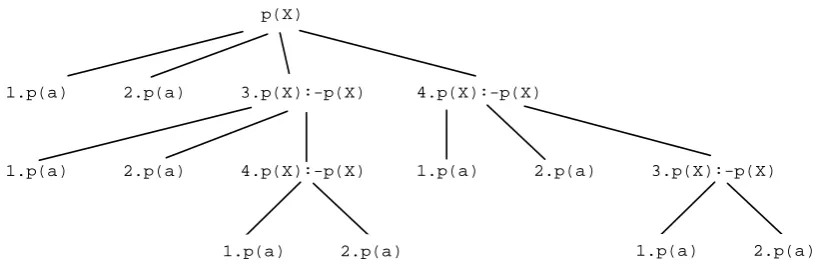
(two facts and a recursive rule, respectively). Its intended meaning is the multiset containing the tuplep(a)four times, where two tuples correspond to the extensional rules forpand the other two to the single intensional rule forp. This intensional rule generates one tuple for each exten-sional rule. By adding the rulep(X) :- p(X)once more, the meaning of pwould contain p(a)ten times, i.e., it contains: two tuples from the two facts, and four tuples for each recursive rule. The first recursive rule is source of four tuples because of the two facts and the two tuples from the second recursive rule (analogously for the second recursive rule). In fact, this mimics SLD resolution by collecting all possible answers coming fromdifferentsources, therefore prun-ing infinite computation paths, i.e., all possible computation paths are considered, stoppprun-ing when a (recursive) node already used in the computation is reached. Figure2shows the tabling tree for the queryp(X)and the annotated program 1.p(a), 2.p(a),3.p(X) :- p(X), and 4.p(X) :- p(X). Infinite computations are elided in this case because the rule with identifier 3is neither reused for solving its body nor the body of rule4as this rule is a descendant of3 (analogously for rule4).
The idea above about uniquely identifying each rule can be applied to recursive predicates
p(X)
1.p(a) 2.p(a) 3.p(X):-p(X) 4.p(X):-p(X)
1.p(a) 2.p(a) 4.p(X):-p(X) 1.p(a) 2.p(a) 3.p(X):-p(X)
1.p(a) 2.p(a) 1.p(a) 2.p(a)
Figure 2: Tabling tree for the queryp(X)
as well. One possible solution is to keep track of the computation path by annotating the rules which have been used to deduce a given atom. So, each entry in the extension table can be identified by a chain of such rule identifiers. Each deduced atom is associated with a pair (Id, IdChain), whereIdis the identifier of the rule which is the generator of the atom, andIdChain is the list of as many pairs as goals in ruleId. So, all rule identifiers in the computation path up to the tabling tree leaf are stored. Referring to Figure2, the following are the entries stored in the extension table after computation, from left to right: (p(a), (1,[])), (p(a), (2,[])), (p(a), (3,[(1,[])])), . . . , (p(a), (4,[(3,[(2,[])])])).
To implement this, two additional parameters to predicatememo/1 are added: Dfor selecting whether or not duplicate answers for a relation are requested (all,distinct, resp.) or elim-inate duplicates for a given set of arguments (distinct(Vs,Ps)), andIdas the identifier pair as described above. Its new prototype ismemo(+G,+D,-Id). These two parameters are passed toet lookup (which is further explained in Subsection5.3) in the first clause of this predicate and also tono subsumed by et(Q,D,(G,Id)), which is modified as follows:
% no_subsumed_by_et(+Query,+Distinct,+(Goal,IdGoal))
no_subsumed_by_et(Q,all,(_G,_IdG)) :- % No entry matching Q \+ et_lookup(Q,all,_IdQ), !.
no_subsumed_by_et(Q,all,(G,IdG)) :- % Existing entries matching Q
nr_id(IdG), % Check that IdG is not cyclic
\+ (et_lookup(Q,all,IdQ), my_subsumes((Q,IdQ),(G,IdG))).
no_subsumed_by_et(Q,_D,(G,_IdG)) :- % For distinct answers
\+ (et_lookup(Q,all,_IdQ), my_subsumes(Q,G)).
5.2 Duplicates and Nulls
listings, which in particular shows null internal representations, in the former case both tuples are listed.
5.3 Duplicate Elimination
When duplicates are enabled, duplicate elimination is provided with the built-indistinct/1, which applies to a positive atom. In this case, duplicate elimination policy for an atomAconsists of discarding all duplicates forA and all of its descendants in the tabling tree. To implement this policy, functionmemois added with a parameter indicating whether duplicates are discarded (distinct) or not (all). When adistinct(G)call is to be solved with predicatesolve, a call to this function is called with this parameter, which is passed to subsequent descendant calls to the memo function in the same subtree. Because there can be other calls toAnot involved in a duplicate elimination path, all its answers are computed by the generator, and consumers in-volved in duplicate elimination are responsible of using non-repeated entries. So, each consumer uses the modified predicateet lookup, as shown next, including a new second parameter se-lecting whether or not all duplicate answers are requested:
% et_lookup(+Goal,+Distinct,-Id)
et_lookup(G,all,IdG) :- et(G,IdG).
et_lookup(G,distinct,IdG)
:-findall((G,IdG),et(G,IdG),GIdGs), setof(G,IdGˆmember((G,IdG),GIdGs),Gs), member(G,Gs), once(member((G,IdG),GIdGs)).
This predicate is called from predicatememo/3 in two scenarios: First, for consumers that get all entries in the extension table for a subsumed call (first clause ofmemo) or from a previous fixpoint iteration (first call in second clause ofmemo), both with the valuedistinctfor the second argument of et lookup. In this first case and when distinct answers are required, second clause ofet lookupis applied. Second case is for generators (second call in second clause ofmemo), where all answers are required and this predicate is called with second argument with all. For providing distinct entries in ET, first all entries matching the input goal are collected with findall, along with their identifiers. Next, setof filters duplicated goals. Each possible answerGis selected withmember via backtracking. One class representant is finally selected with the only one solution call to member in last line. Its identifier of this representant is the one returned.
5.4 Duplicates and Projection
Aforementioned handling of duplicate elimination is not enough to deal with correlated SQL queries. Compiling such a SQL query to Datalog may involve a distinct operator for a projection (a subset) of the arguments in a relation as, for instance:
CREATE TABLE t(a int, b int); CREATE TABLE s(a int, b int);
CREATE VIEW v(a) AS SELECT a FROM t WHERE a IN (SELECT DISTINCT a FROM s WHERE t.b<s.b);
A possible Datalog program for this view follows:
v(A) :- t(A,B), distinct(v_1(A,B)).
But this is not a correct equivalent formulation because distinct/1 applies to different tuples fromv_1instead of different values fora, andbmust be passed tov_1to filter results. So, a new built-indistinct(Arguments,Relation)is needed, which computes different results for the list of relation arguments for the relation. The first Datalog rule would be rewritten asv(A) :- t(A,B), distinct([A],v 1(A,B)).
Solving this new built-in is via the callmemo(G,distinct(Vs,Ps),Id), whereGis to be computed for returning only distinct tuples of variablesVs, which correspond to argument positionsPs. These positions are kept to account projection positions as any variable inVsmight become ground before solving this call. no_subsumed_by_et/3 is modified accordingly by adding the next clause, which deals with duplicate elimination when duplicates are enabled.
no_subsumed_by_et(Q,distinct(_Vs,Ps),(G,_IdG)) :-\+ (functor(Q,F,A), functor(FQ,F,A),
get_ith_arg_list(Ps,Q,QAs), get_ith_arg_list(Ps,FQ,QAs), et(FQ,_Id),get_ith_arg_list(Ps,G,GAs),my_subsumes(QAs,GAs)).
As well, predicateet_lookup/3 is added with the following clause:
et_lookup(G,distinct(Vs,_SG),IdG)
:-findall((G,IdG),et(G,IdG),GIdGs), term_variables(G,GVs), set_diff(GVs,Vs,EVs),
build_ex_quantifier(EVs,my_member((G,IdG),GIdGs),QG),
setof(Vs,IdGˆQG,Vss), my_member(Vs,Vss), once(my_member((G,IdG),GIdGs)).
Although similar to the second clause of this predicate in previous section, this clause adds handling of unprojected variables by building existential quantifiers over them, so thatsetof/3 returns distinct tuples for projected variables.
5.5 Duplicates in Aggregates
Aggregates are supported in DES in several flavors [SP11], both as functions and predicates, but for the sake of this paper, we restrict the presentation to a simplified aggregate predicates. An ag-gregate predicate returns its result in its last argument position, as insum(p(X),X,R), which binds Rto the cumulative sum of values for X, provided by relation p. Duplicate elimination versions are also available, such assum distinct/3.
Solving rules involving aggregates via successive fixpoint iterations might lead to incorrect entries to be added to the extension table because in a given iteration it is not ensured that all the meaning of the aggregated relation is computed. A straightforward approach to solve them is analogous to negation: new negative arcs are added to the dependency graph in order to place such relation in a stratum lower than the predicate of the rule in which it occurs. So, the rule s(R) :- sum(p(X),X,R)implies an arc s←¬p, which in turn also implies the constraint strata(p)<strata(s)for the stratification.
compute_distinct_aggregate_pred(Aggr)
:-Aggr =.. [F,R,V,O], R =.. [_P|Args], get_arg_position(V,Args,I), nf_setof(N, CRˆIdsˆ(et(CR,Ids),\+ \+ (CR=R),
arg(I,CR,N),N\=’$NULL’(_Id)), Ns), compute_aggregate(F,Ns,O).
Here, nf setof is the non-failing version of setof (it returns an empty list instead of failure), and collects all values for the argument to which the aggregate is applied (X in the example above). As in relational databases, null arguments are omitted from this set.
6
Enhancing Performance
Several performance penalties can be found in the current implementation of the deductive database system DES. Next, we list them and propose some ways for overcoming:
• Prolog-based implementation. Instead of resorting to a compiler generating native code, we have used a Prolog system because it is much more adequate for rapid prototyping than low-level languages as, e.g., C++. Indeed, the higher abstraction level of Prolog w.r.t. third generation languages is a definitive advantage to quickly get results. However, one can find speed-ups in such languages which are orders of magnitude better. Even Java programs compiled to byte code, reveal better performance, as, e.g., the classic queens benchmark if compared to a CLP(FD) implementation.
• Interpreted vs. compiled Prolog code. We assert Datalog rules in a dynamic Prolog database. Most Prolog systems distinguish between asserted and compiled (consulted) programs. Whereas the former use the dynamic database, the latter compile to some sort of WAM code including first-argument indexing. This makes consulted programs perform better than asserted programs. So, following [Die87], we could implement query solving in the definition of Datalog predicates and queries. Then, predicates would be compiled instead of asserted and therefore more efficient.
• Indexing. Despite the last issue and its improvement, there remains dynamic data in the call and extension tables. On the one hand, such dynamic data suffers from the same issue as above, and, on the other hand, accessing such data structures with a sequential index is not enough for large amounts of data (assuming that we could automatically do it as the Prolog compiler does with compiled predicates). Better index structures should be taken into account, such as balanced trees or, better,tries, as implemented in the XSB system.
7
Conclusions
This paper has shown how some widespread-used features in relational databases, namely nulls, outer joins and duplicates, can be included altogether into a tabled deductive database system. Since this system compiles SQL statements to Datalog programs, it was a need to embody such features coming from relational database systems into the concrete deductive inference engine DES. Because this system is not geared towards performance, this implementation should be seen as a proof of concept. Some hints have been provided for the porting to other deductive systems and future work may include to use other external efficient engines such as XSB.
Bibliography
[BD98] G. Brewka, J. Dix. Knowledge Representation with Logic Programming. In Dix et al. (eds.),Proceedings of LPKR’97. LNAI 1471, pp. 1–51. Springer-Verlag, 1998.
[CGS08] R. Caballero, Y. Garc´ıa-Ruiz, F. S´aenz-P´erez. A Theoretical Framework for the Declarative Debugging of Datalog Programs. InInternational Workshop on Seman-tics in Data and Knowledge Bases. LNCS 4925, pp. 143–159. Springer, 2008.
[CGS10] R. Caballero, Y. Garc´ıa-Ruiz, F. S´aenz-P´erez. Applying Constraint Logic Program-ming to SQL Test Case Generation. InProc. International Symposium on Functional and Logic Programming (FLOPS’10). LNCS 6009. 2010.
[CGS11] R. Caballero, Y. Garc´ıa-Ruiz, F. S´aenz-P´erez. Algorithmic Debugging of SQL Views. InErshov Informatics Conference (PSI’11). LNCS. Springer, 2011. In Press.
[Dam96] C. Dam´asio. Paraconsistent Extended Logic Programming with Constraints,. PhD thesis, Dept. de Informˆatica, Universidade Nova de Lisboa, 1996.
[Dat09] C. J. Date. SQL and relational theory: how to write accurate SQL code. O’Reilly, Sebastopol, CA, 2009.
[Die87] S. W. Dietrich. Extension Tables: Memo Relations in Logic Programming. InIEEE Symp. on Logic Programming. Pp. 264–272. 1987.
[GCH+08] P. C. de Guzm´an, M. Carro, M. V. Hermenegildo, C. Silva, R. Rocha. An improved continuation call-based implementation of tabling. PADL’08, pp. 197–213, 2008.
[LAC99] J. Y. Liu, L. Adams, W. Chen. Constructive negation under the well-founded seman-tics.JLP38(3):295–330, 1999.
[LPF+06] N. Leone, G. Pfeifer, W. Faber, T. Eiter, G. Gottlob, S. Perri, F. Scarcello. The DLV system for knowledge representation and reasoning. ACM Tran. on Computational Logic7(3):499–562, 2006.
[RU93] R. Ramakrishnan, J. Ullman. A survey of research on Deductive Databases. JLP 23(2):125–149, 1993.
[SP11] F. S´aenz-P´erez. DES: A Deductive Database System.Electronic Notes on Theoretical Computer Science271:63–78, March 2011.
[SP12a] F. S´aenz-P´erez. Datalog Educational System. May 2012.http://des.sourceforge.net/.
[SP12b] F. S´aenz-P´erez. Outer Joins in a Deductive Database System. Electronic Notes in Theoretical Computer Science282:73 – 88, 2012.
[SD91] C. Shih, S. Dietrich. Extension Table Evaluation of Datalog Programs with Negation. InProc. of the IEEE International Phoenix Conference on Computers and Commu-nications. Volume AZ, pp. 792–798. Scottsdale, March 1991.
[SS06] Z. Somogyi, K. Sagonas. Tabling in mercury: Design and implementation. In In Proceedings of Practical Aspects of Declarative Programming (PADL’06). Pp. 150– 167. Springer-Verlag, 2006.
[SSW94a] K. Sagonas, T. Swift, D. S. Warren. XSB as an Efficient Deductive Database Engine. InIn Proceedings of the ACM SIGMOD International Conference on the Manage-ment of Data. Pp. 442–453. ACM Press, 1994.
[SSW94b] K. Sagonas, T. Swift, D. S. Warren. XSB as an efficient deductive database engine. InSIGMOD’94: Proceedings of the 1994 ACM SIGMOD International Conference on Management of Data. Pp. 442–453. ACM, New York, NY, USA, 1994.
[SW10] T. Swift, D. S. Warren. XSB: Extending Prolog with Tabled Logic Programming. CoRRabs/1012.5123, 2010. Submitted to TPLP.
[SWSJ09] T. Swift, D. Warren, K. Sagonas, J. Freire et al. The XSB System Version 3.2. Volume 2: Libraries, Interfaces and Packages. 2009.
[TG94] B. Traylor, M. Gelfond. Representing Null Values in Logic Programming. In LFCS’94. Pp. 341–352. 1994.
[TS86] H. Tamaki, T. Sato. OLDT Resolution with Tabulation. InThird International Con-ference on Logic Programming. Pp. 84–98. 1986.
[Ull88] J. D. Ullman. Database and Knowledge-Base Systems, Vols. I (Classical Database Systems) and II (The New Technologies). Computer Science Press, 1988.
[ZCF+97] C. Zaniolo, S. Ceri, C. Faloutsos, R. T. Snodgrass, V. S. Subrahmanian, R. Zicari. Advanced Database Systems. Morgan Kaufmann, 1997.