Model-based shape matching of orthopaedic implants in RSA and fluoroscopy

(1)

The handle

http://hdl.handle.net/1887/33103

holds various files of this Leiden University

dissertation

Author: Prins, A.H.

Title:

Model-based shape matching of orthopaedic implants in RSA and fluoroscopy

(2)

Model-based shape matching

of orthopaedic implants

in RSA and fluoroscopy

(3)

Cover design and Layout: A.H.Prins

(4)

Model-based shape matching

of orthopaedic implants

in RSA and fluoroscopy

Proefschrift

ter verkrijging van

de graad van Doctor aan de Universiteit Leiden, op gezag van Rector Magnificus prof. mr. C.J.J.M. Stolker,

volgens besluit van het College voor Promoties te verdedigen op

donderdag 4 juni 2015 klokke 16:15 uur

door

Anne Hendrik Prins

(5)

Promotor: Prof. dr. ir. E.R. Valstar Co-promotores: Dr. ir. B.L. Kaptein

Dr. B.C. Stoel

Overige leden: Prof. dr. R.G.H.H. Nelissen Prof. dr. ir. J.H.C. Reiber

Prof. dr. J. Harlaar (VUMC, Amsterdam)

(6)

(7)

(8)

CONTENTS

1 Introduction 1

1.1 Radiological assessment of implant position and kinematics . 2

1.2 Aim . . . 7

2 Integrated contour detection 9 2.1 Introduction . . . 11

2.2 Method . . . 12

2.3 Validation: experimental . . . 15

2.4 Validation: clinical . . . 17

2.5 Results: experimental . . . 18

2.6 Results: clinical . . . 19

(9)

3.1 Introduction . . . 27

3.2 Methods . . . 28

3.3 Experimental setup . . . 31

3.4 Results . . . 33

3.5 Discussion . . . 35

4 Detecting femur-insert collisions 41 4.1 Introduction . . . 43

4.2 Methods . . . 44

4.3 Experimental setup . . . 47

4.4 Results . . . 49

5 Performance of optimization 57 5.1 Introduction . . . 59

5.2 Methods . . . 60

5.3 Experiments . . . 66

5.4 Results . . . 68

(10)

6 Detecting condylar contactloss 77

6.1 Introduction . . . 79

6.2 Methods . . . 81

6.3 In vivo experiment . . . 83

6.4 Phantom experiments . . . 85

6.5 Results . . . 87

7 Discussion and recommendations 95 7.1 Recommendations . . . 99

8 Summary 103

9 Samenvatting 107

References 111

List of publications 123

Curriculum 125

(11)

(12)

CHAPTER

1

(13)

1.1 Radiological assessment of implant position

and kinematics

In patients with severe arthritis, e.g. osteoarthritis or rheumatoid arthritis, the replacement of the degenerated joint by a prosthesis is a common and successful surgical procedure. Approximately ninety percent of the implants will function well for up to 15 years, greatly alleviating pain and improving the function of the joint [Gill et al., 1999, Kim et al., 2001, Costigan et al., 2002, Malchau et al., 2002, Banks et al., 2003, Catani et al., 2006, Havelin et al., 2009]. However, some implants fail much earlier, e.g. due to an infection or dislocation, but most commonly due to aseptic loosening. As a consequence another major surgery is eventually needed to replace the implant.

Radiolucency measured on standard clinical radiographs has been shown to be an important indicator of implant loosening. However, radiolucency is an indirect measure of possible prosthesis loosening and it can be underesti-mated on a radiograph or can be difficult to measure due to overprojection [Nelissen, 1995, Reading et al., 1999]. The migration of the implant over time with respect to the bone is an alternative measurement of implant loosening.

(14)

Introduction

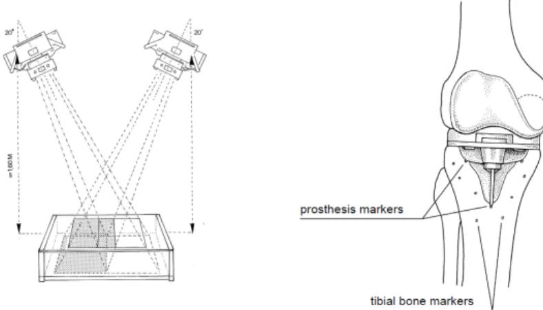
Figure 1.1: Typical RSA setup with two Roentgen foci (left) and a schematic of a knee implant with markers in the surrounding bone (right)

Where implant position is measured to assess migration, the measurement of in vivoimplant motion is an important tool for validating the implant design by comparing actual in vivo implant motion with its designed movements. The external limb motion is often measured with a motion capture system which measures the positions of small markers attached to the skin with multiple camera’s. However, the measurement of implant motion is inaccu-rate using external motion capture, because the skin and attached markers move relative to the implant [Sati et al., 1996, Leardini et al., 2005, Garling et al., 2007, Barre et al., 2013]. In addition, such external measurements cannot measure the internal kinematics of for example the mobile bearing in a knee implant [Garling et al., 2005, Wolterbeek et al., 2009, 2012a].

(15)

1.1.1 Model-based RSA

At the Leiden University Medical Center, RSA software has been developed with a model-based approach to determine the implant position and orien-tation from stereo radiographs (Model-based RSA) [Valstar, 2001, Kaptein et al., 2003]. Without the need for attaching markers to the implant, model-based RSA determines the position and orientation of the implant from the shape of its silhouette in the radiographs. Markers are still necessary in the bone as model-based matching of the bone is not yet accurate enough.

The outer contour of the implant silhouette is extracted from the X-ray image and shape matching determines the position and orientation of an accurate 3D model of the implant, such that a virtual projection of a 3D model of the implant matches the implant silhouette. Computer-aided de-sign (CAD) implant models were initially used for Model-based RSA, but the accuracy of a reverse-engineered (RE) model was shown to increase the accuracy of Model-based RSA [Kaptein et al., 2003]. In clinical practice, the relative position and orientation of the implant can be measured with errors smaller than 0.5 mm and 0.5◦ [Kaptein et al., 2006]. The method has been applied successfully in clinical studies to measure implant position and migration [Nelissen et al., 2005, 2002, Nieuwenhuijse et al., 2012, Pijls et al., 2012].

A possible limitation of model-based RSA is introduced, where the specific shape of the implant model makes model-based shape matching in some cases infeasible or inaccurate. Shape matching relies on a sufficiently unique silhouette such that the implant position and orientation can be determined. For example, rotating a hip stem about its longitudinal axis results in no changes or minor changes to its silhouette due to its cylindrical shape. This makes the measurement of this longitudinal rotation inaccurate.

1.1.2 Model-based fluoroscopic analysis

(16)

kinemat-Introduction

ics [Garling et al., 2005, Wolterbeek et al., 2009, 2012a,b]. A few mile-stone papers were published halfway the nineties on measuring knee implant kinematics utilizing single-plane fluoroscopy [Stiehl et al., 1995, Banks and Hodge, 1996]. Stiehl et al. [1995] measured the knee kinematics of 47 pa-tients by estimating the position and orientation of the implant in static radiographs every 5◦ of knee flexion. Banks and Hodge [1996] demonstrated the feasibility of fluoroscopy, or X-ray video, to record knee kinematics. Similar methods have been developed for measuring the position and ori-entation of the implant for model-based fluoroscopic analysis [Zuffi et al., 1999, Mahfouz et al., 2003, Komistek et al., 2003, Kanisawa et al., 2003, Li et al., 2004, Hermans et al., 2007, 2008].

The estimation of the position and orientation of the implant has been done using features, intensities or gradients [Markelj et al., 2012]: feature-based methods perform pose estimation on features extracted from the image such as the outer contour of the implant’s silhouette. Intensity-based or gradient-based methods perform the estimation directly on the image data or after edge detection in the image.

The feature-based approach for fluoroscopic analysis has been further devel-oped in this thesis. The features of the implant silhouette are detected in the X-ray video frame. A model-based shape matching approach, similar to the one used in model-based RSA, estimates the position and orientation of a 3D implant model. An optimization method minimizes an error measure, such that a virtual projection of a 3D model of the implant matches the implant silhouette.

(17)

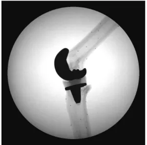
Figure 1.2: Typical high quality fluoroscopic frame of a phantom experiment

However, poor accuracy with errors of several millimeters has been reported for the out-of-plane position due to the single-plane nature of fluoroscopic analysis [Banks and Hodge, 1996, Hoff et al., 1998, Mahfouz et al., 2003, Komistek et al., 2003, Kanisawa et al., 2003]. With fluoroscopic analysis of a knee implant, this can result in the femoral component seemingly inter-secting with the polyethylene insert, which is physically impossible.

As another limitation, the resolution and contrast of fluoroscopic frames are much lower compared to clinical radiographs and large image deformation is present on analogue systems with image intensifiers. When capturing a dynamic task with a high frame rate, a compromise needs to be found between exposure time, X-ray intensity, pulse width and radiation exposure for the subject. Such a compromise may result in poor image quality, which makes it difficult to distinguish the implant silhouette from the surrounding bony structures and tissues in the frame.

(18)

Introduction

The labour-intensive nature makes model-based shape matching operator-dependent and possibly less robust. The number of frames to be analyzed after a single session can run into the hundreds or thousands when a captured dataset can easily encompass a few seconds of video with frame rates up to 30 Hz. This makes the analysis time-consuming and limits the method to small scale study groups.

1.2 Aim

Model-based shape matching methods for RSA and fluoroscopy are valuable for measuring implant migration and implant kinematics. However, several limitations have been described in the reliability and usability of such meth-ods. Therefore, the aim of this research is to improve the reliability and usability of model-based shape matching for RSA and fluoroscopic analysis. Therefore, current limitations have been investigated in this thesis and new approaches have been developed:

Improvements to the interactivity of the shape matching method: The labour-intensive nature of model-based shape matching makes the method operator-dependent and possibly less robust. The selection of relevant contour parts needs to be done manually and the researcher needs to review the results of pose estimation each frame and restart the process in case of suboptimal solutions.

A new model-based shape matching method will be presented with in-tegrated contour detection, which improves the interactivity and ease-of-use of the algorithm, thereby making the pose measurements more robust and less operator dependent when dealing with poor image quality (Chapter 2).

(19)

A combined model approach to improve the accuracy: The specific shape of the implant model could cause a failure in model-based shape matching or limit the accuracy. For example, rotating a hip stem about its longitudinal axis results in no changes or minor changes to its sil-houette due to its cylindrical shape. This makes the measurement of this longitudinal rotation inaccurate.

A solution will be presented in Chapter 3 for increasing the accuracy of pose estimation for hip stems by adding the spherical head to the model with an additional degree of freedom.

In Chapter 4 the out-of-plane accuracy in single-plane fluoroscopy is improved by combining the femoral and tibial component into a single model. By adding a collision constraint, physically impossible inter-sections between the femoral component and the polyethylene insert are prevented.

(20)

CHAPTER

2

INTEGRATED CONTOUR DETECTION AND POSE

ESTIMATION FOR FLUOROSCOPIC ANALYSIS OF KNEE IMPLANTS

A.H. Prins1_{, B.L. Kaptein}1_{, B.C. Stoel}2_{, R.G.H.H. Nelissen}1_{, J.H.C. Reiber}2_{, E.R. Valstar}1,3 1. Biomechanics and Imaging Group, Department of Orthopaedics, Leiden University Medical Center, The Netherlands

2.Division of Image Processing, Department of Radiology, Leiden University Medical Center, The Netherlands

3. Department of Biomechanical Engineering, Faculty of Mechanical, Maritime and Materials Engineering, Delft University of Technology, The Netherlands

Proceedings of the Institution of Mechanical Engineers, Part H: Journal of Engineering in Medicine

(21)

Abstract

With fluoroscopic analysis of knee implant kinematics the implant contour must be detected in each image frame, followed by estimation of the implant pose. With a large number of, possibly low quality, images, the contour de-tection is a time-consuming bottleneck. In this article anAutomatedcontour detection method is proposed, which is integrated in the pose estimation.

In a phantom experiment theAutomated method was compared to a Stan-dard method, which uses manual selection of correct contour parts. Both methods demonstrated comparable precision, with a minor difference in the Y-position (0.08 mm vs. 0.06 mm). The precision of each method was so small (below 0.2 mm and 0.3◦) that both are sufficiently accurate for clinical research purposes.

The efficiency of both methods was assessed on six clinical datasets. With the Automated method the observer spent 1.5 minutes per image, signifi-cantly less than 3.9 minutes with the Standard method. A Bland-Altman analysis between the methods demonstrated no discernable trends in the relative femoral poses.

(22)

Integrated contour detection

2.1 Introduction

Single-plane fluoroscopic analysis is an important tool for the evaluation of knee implant kinematics. Many methods have been described for the estimation of the three-dimensional (3D) position and orientation (pose) of the implant in each fluoroscopic image. Template-matching [Banks and Hodge, 1996, Hoff et al., 1998] or model-based 3D-to-2D registration [Zuffi et al., 1999, Kaptein et al., 2003] are common approaches. These methods have accuracies ranging from 0.09 mm to 0.40 mm for the in-plane positions and from 0.35◦ to 1.3◦ for the orientations [Banks and Hodge, 1996, Hoff et al., 1998, Mahfouz et al., 2005, Komistek et al., 2003, Kanisawa et al., 2003, Li et al., 2004, Garling et al., 2005, Hanson et al., 2006]. These in-plane accuracies are sufficient for clinical uses, whereas the out-of-plane position is considered not accurate enough for usage in many clinical applications.

Many of these methods require that the contour of the implant is detected in each image frame. The implant pose is then estimated by minimizing the difference between the contour and a virtual projection of the model. Contour detection is often a manual or semi-automatic task, which requires a significant amount of user interaction: selecting the relevant contour parts or discarding the erroneous parts. Since fluoroscopic images have lower image contrast and resolution than standard X-rays and the contour detection must be performed for each single image in a dataset, this makes the analysis cumbersome and time-consuming. In addition, the accuracy of the detected contour is an important factor in the final accuracy of the estimated pose [Fregly et al., 2005, Mahfouz et al., 2005]. Because Mahfouz et al. [2005] considered contour detection too prone to errors, they suggested to avoid an a priori contour detection step and instead use a direct model-to-image pose estimation method.

(23)

one image to the next [Zuffi et al., 1999].

Both phantom and clinical data were used to validate the accuracy and precision on the clinically relevant in-plane positions and orientations. It is compared to a conventional model-based pose estimation method [Kaptein et al., 2003] with semi-automatic contour detection (the Canny edge detector [Canny, 1986]), and the effects of image quality, the agreement in pose and the analysis time of the methods were investigated as well.

2.2 Method

The main input of the automated model-based contour detection method consists of a fluoroscopic image, the relative X-ray focus position and a 3D surface model of the implant. Furthermore, an initial candidate pose is required.

The image is preprocessed by applying noise reduction with a Gaussian filter. The integrated pose estimation and contour detection consist of the following loop (Algorithm 1), updating the contour and pose in each iteration:

Algorithm 1 Pose estimation with integrated contour detection

1: for each iteration do 2: Detection:

Model-based contour detection, based on the current candidate pose. 3: Selection:

Contour-point selection, automatically selecting 20% of the (good-quality) contour parts.

4: Pose estimation:

Robust pose estimation with the selected contour parts, giving a new candidate pose.

(24)

The initial pose for the method can be provided by the user. For example, in our application the user can easily and intuitively manipulate the 3D surface model and can get direct feedback of the implant pose with respect to the image. A second possibility is the propagation of the implant pose from the analysis of an earlier image frame [Zuffi et al., 1999], and this allows for the automatic analysis over all image frames.

2.2.1 Model-based contour detection

First, a virtual projection of the model onto the image plane is calculated (Figure 2.1a) [Kaptein et al., 2003]. This projection is a closed curve and represents the outer boundary of the implant silhouette.

A region of the image around the virtual projection is then resampled along scan lines perpendicular to the virtual projection (counterclockwise and from outside to inside). The resulting scan-matrix represents a straightened ver-sion of the image region in a band around the virtual projection. Each line in the matrix corresponds to a scan line starting at the outside of the virtual projection and ending on the inside of the virtual projection (Figure 2.1b). The width of this region can be adjusted by setting the length of the scan lines; the pixel spacing is the same as in the original image.

A derivative matrix is calculated with a convolution operation ( [1 0 −1] kernel) along each line in the intensity matrix. This represents the derivative in the image perpendicular to the virtual projection. With a dark implant silhouette, the positive edges (from black to white) will be assigned a high value, while negative edges (from white to black) a low value (Figure 2.1c).

A dynamic programming approach extracts an optimal path, passing each scan line once, while maximizing the sum of edge values in the edge matrix [Bellman and Dreyfus, 1966]. The resulting path follows decreasing edges (from white to black) as close as possible (Figure 2.1c). This path is trans-formed back into the image domain (Figure 2.1d) and for each point the edge strength (derivative edge value) is stored.

(25)

Figure 2.1: a) Contour detection starts with a virtual projection. b) The im-age is resampled (counter-clockwise) along this virtual projection with scan-lines perpendicular to the projection, resulting in a scan-image with the virtual pro-jection as a straight line in the center (dashed line) and the corresponding scan lines. c) A convolution with a positive difference filter ([-1 0 1]) results in the cost-image (third image). Minimal path extraction using dynamic programming then extracts a path (dashed curve). d) After back-transforming this path, the result is a contour (right image) with associated edge strengths.

around the virtual projection, with the edge strengths available for later use by the pose estimation.

2.2.2 Contour-point selection

The edge strengths are normalized over the entire contour to a range of [0,1]. Using a threshold in the range of [0,1], the user can specify how much of the contour should be discarded. Contour points with an edge strength below the threshold are then discarded (a threshold of 0.25 was typically used). From the remaining contour-points (those with an edge strength above the threshold), 20% was selected, uniformly sampled along the contour, in order to reduce the computational cost.

2.2.3 Robust pose estimation

(26)

To this end, a weighted distance measure is calculated between the selected contour points and the virtual projection of the implant model. The distance measure is the same as described by Kaptein et al. [Kaptein et al., 2003], with one addition: The edge strengths from the selected contour points are used as weights.

2.3 Validation: experimental

Data was collected from a phantom experiment using a bi-plane flat panel fluoroscopic setup (Super Digital Fluoroscopy (SDF) system, Toshiba In-finix: Toshiba Medical Systems Europe, Zoetermeer, The Netherlands). The phantom study was performed with a size 3 cruciate-substituting PFC-Sigma prosthesis fixed in sawbones with a 5 mm thick insert (DePuy Orthopedics, Warsaw, IN). A 3D implant model of the femoral component was reverse engineered with an accuracy of 0.05 mm (TNO Industry, Eindhoven, The Netherlands) for use by the pose estimation methods.

The image intensifiers were positioned perpendicular to each other and the sawbones were placed such that one image intensifier had a medial-lateral view, while the other had an anterior-posterior view. The X-ray focus posi-tions were calculated using a calibration box [Koning et al., 2007].

Two motions of the femur were captured (15 fps). In the first motion, the femur moved from full extension to 90◦ of flexion, followed by an abduction of approximately 20◦, back to 20◦ adduction and finally back to full exten-sion. In the second motion, the femur started at 30◦ of flexion, moved to full extension after which some internal/external rotation (roughly 20◦) was performed.

(27)

2.3.1 Image quality

The new method was validated on single-plane fluoroscopic image data using the data from the phantom experiment, but only from the image intensifier with a medial-lateral view. This data was of excellent quality; high resolu-tion and high image contrast. In routine clinical practice, the image quality is worse and can have an influence on the accuracy of contour detection and pose estimation. In this validation experiment the effects of lower image quality on the new method was investigated.

The image qualities were assessed as encountered in ongoing clinical studies. Four quality levels were defined: L0,L1,L2 andL3. LevelL0 has no quality reduction and serves as a baseline measurement. LevelsL1 - L3 represent good, moderate and poor qualities, respectively. Each image was degraded according to these levels with the following method:

1. A template image was created with Simplex noise [Perlin, 2001] which was used as a template for local intensity-reduction. This resulted in different parts of the image having different intensity levels, which was used to crudely simulate different contrasts, which can arise in clinical practice due to soft tissue.

2. Locally varying Gaussian noise was introduced and the overall sharp-ness of the image was reduced with a Gaussian blur.

The parameters used, the example images and the corresponding clinical images are presented in Figure 2.2

(28)

optimiza-Integrated contour detection

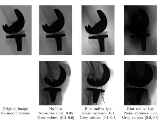
Original image No blur Blur radius 1px Blur radius 1px

No modifications Noise variance: 0.05 Noise variance: 0.1 Noise variance: 0.2 Grey values: [0.2,0.6] Grey values: [0.1,0.4] Grey values: [0.0,0.3]

Figure 2.2: Examples of reduced quality images of the phantom experiment in the first row and their clinical counterparts on the second row. The intensity-range on a scale of[0,1]is presented for each image in the third row, together with the variance for the noise.

tion of the distance measure between the contour points and the implant model [Kaptein et al., 2003].

For both the Automated and the Standard method, the error in pose was calculated as the difference for each pose-parameter with respect to the pose obtained by the bi-planeReference measurement. Students T-test was then used to compare the mean errors between theStandard and theAutomated and Levene’s test to compare the variance of the differences.

2.4 Validation: clinical

(29)

were considered of moderate quality, while those of the other patient were considered of good quality, comparable to levelsL1 and L2 in Figure 2.2.

An experienced user applied both the Automated and Standard methods to each dataset and the total analysis time was recorded for each method. The tibial and femoral components were analyzed and the relative poses between the two components were calculated for each method. To deter-mine the agreement between the two methods, a Bland-Altman analysis was performed for each pose parameter.

2.5 Results: experimental

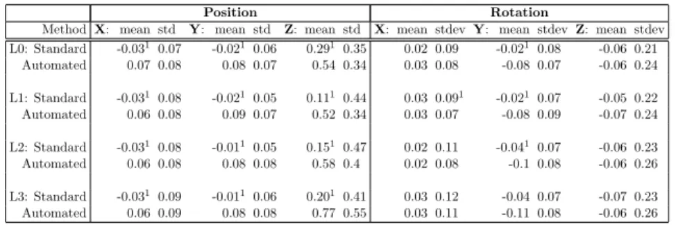
All the errors in pose for both methods are presented in Table 2.1. The mean errors and the standard deviations for the highest and lowest image qualities (L0 andL3) are presented in Figure 2.3. The most prominent differences are in the systematic errors between the two methods: TheAutomated method demonstrates small, but statistically significant worse systematic errors in the in-plane positions (X: 0.07 mm, Y: 0.08 mm), which is consistent over all quality levels. The mean error in the less accurate out-of-plane position increases up to 0.77 mm for theAutomatedmethod and is significantly larger (p <0.001) than theStandard method for all quality levels.

(30)

Figure 2.3: Standard deviations of the error in pose with respect to the reference pose measurement for the Automated and Standard methods and the best and the worst level of image quality.

2.6 Results: clinical

On average an experienced user spent 3.9±0.36 minutes per image with the Standard method, whereas the Automated required only 1.5±0.36 minutes per image. This difference was highly significant (p <0.001).

The Bland-Altman plots of the relative pose with respect to the tibia pose are presented in Figure 2.4. There were no strong trends discernable in the Bland-Altman plots. The largest differences presented themselves in the out-of-plane position with a mean difference of 0.77 mm and large stan-dard deviation of 3.46 mm. A relatively large discrepancy in the Y- and Z-orientation was found with standard deviations of 1.11◦ and 0.98◦.

2.7 Discussion

(31)

Position Rotation

Method X: mean std Y: mean std Z: mean std X: mean stdevY: mean stdevZ: mean stdev L0: Standard -0.031 _0.07 _-0.021_0.06 _0.291 _0.35 _{0.02 0.09} _-0.021 _0.08 _{-0.06 0.21}

Automated 0.07 0.08 0.08 0.07 0.54 0.34 0.03 0.08 -0.08 0.07 -0.06 0.24 L1: Standard -0.031 _0.08 _-0.021_0.05 _0.111 _0.44 _{0.03 0.09}1 _-0.021 _0.07 _{-0.05 0.22}

Automated 0.06 0.08 0.09 0.07 0.52 0.34 0.03 0.07 -0.08 0.09 -0.07 0.24 L2: Standard -0.031 _0.08 _-0.011_0.05 _0.151 _0.47 _{0.02 0.11} _-0.041 _0.07 _{-0.06 0.23}

Automated 0.06 0.08 0.08 0.08 0.58 0.4 0.02 0.08 -0.1 0.08 -0.06 0.26 L3: Standard -0.031 _0.09 _-0.011_0.06 _0.201 _0.41 _{0.03 0.12} _{-0.04 0.07} _{-0.07 0.23}

Automated 0.06 0.09 0.08 0.08 0.77 0.55 0.03 0.11 -0.11 0.08 -0.06 0.26

1

Significant difference (p <0.05) between the Automated and the Standard methods on the same level of image quality.

Table 2.1: Means and standard deviations of the errors in position and orien-tation for both the Automated and Standard methods on single-plane data, with respect to the Reference method (from bi-plane data). The single-plane data was reduced according to four quality levels.

contour detection enables a more intuitive and thus faster analysis proce-dure for the researcher, with only minor consequences for the accuracy of the system. Although the systematic errors of the Automated method are consistently higher than the errors of theStandard method, their values in the clinically relevant parameters remain below 0.1 mm and 0.1◦. In addi-tion, the systematic errors are less important than the standard deviations when investigating implant kinematics, where the relative motions of the components are considered. With respect to the standard deviations, the two methods performed virtually identical. The only significant difference (0.08 mm vs. 0.06 mm) was found in the Y-position. These differences are, however, clinically irrelevant.

(32)

Figure 2.4: Bland Altmann plots for the agreement in the pose measured by the Standard method and the Automated method on the clinical data. The x-axes represent the agreement in the pose parameters, calculated as the mean of the two methods. The y-axes represent the difference in pose-parameter between the two methods. The colors represent the two patients from which the data was obtained. The central dashed line represents the mean difference over all measurements, while the two outer dashed lines indicate limits of agreement for the differences (two standard deviations around the mean).

Automated methods. The difference in contour detection method between the Standard and Automated methods may then cause the discrepancy in the systematic errors between the Standard and Automated methods.

The results from the phantom experiment compare well with the results pub-lished in the literature and are more accurate than the literature. Earlier studies on single-plane fluoroscopy have reported precisions for estimating positions from 0.09 mm to 0.46 mm and precisions for estimating the orien-tations between 0.35◦ and 1.3◦ [Banks and Hodge, 1996, Hoff et al., 1998, Mahfouz et al., 2005, Komistek et al., 2003, Kanisawa et al., 2003]. Fregly et al. (2005) have demonstrated the effects of X-ray attenuation on the accu-racy of the silhouette in the image and how this could possibly account for most of measurement bias. Mahfouz et al. (2005) demonstrated how manual segmentation can severely affect the accuracy of pose estimation and even recommended a pose estimation process without manual, a priori segmenta-tion. TheAutomated method has no such ”manual, a priori segmentation”, but instead relies on an automatic model-based segmentation method.

(33)

analysis-time with theAutomatedmethod with the added advantage that no continu-ous supervision by the researcher was required. With a fluoroscopic dataset of 50 images, a researcher would spend 75 minutes with the newAutomated method, and 195 minutes with theStandard method.

The lack of a good reference measurement in the clinical data makes it dif-ficult to determine the accuracy of the two methods. The two methods show differences within 1 mm and 1◦ for all orientations and positions, re-spectively, except for the out-of-plane position where the differences can be as high as 7 mm. These values are comparable with the earlier mentioned ranges from the literature.

A difficult problem arose with the tibial orientation in three of the six datasets. For several images, there was some ambiguity in the silhouette of the tibial component. Its silhouette was such that both pose estimation methods had to choose from two or sometimes three pose candidates. In those cases it could be that the Standard and Automated picked different pose candidates, resulting in differences in measured orientations of a few de-grees. This is likely an issue with any pose estimation method and could have caused the relatively large differences in Y-orientation and Z-orientation.

When dealing with patient-data, the motion between two consecutive images can be large. Extrapolation of the pose from one image to the next [Zuffi et al., 1999] can then put the implant model too far away from its new silhouette. This can cause the automatic model-based contour detection to fail, when the detection region on the image around the virtual projection of the model is too small to capture enough parts of the new contour. To overcome this problem, the detection region can be enlarged. However, this adds the risk that another strong contour instead of the implant contour is found, e.g. the skin-to-air transition. In those cases it was easier for the user to update the model pose interactively and then continue the analysis.

(34)

a threefold reduction in analysis time.

2.7.1 Acknowledgement

(35)

(36)

CHAPTER

3

HANDLING MODULAR HIP IMPLANTS IN MODEL-BASED RSA: COMBINED STEM-HEAD MODELS

A.H. Prins1_{, B.L. Kaptein}1_{, B.C. Stoel}2_{, R.G.H.H. Nelissen}1_{, J.H.C. Reiber}2_{, E.R. Valstar}1,3 1. Biomechanics and Imaging Group, Department of Orthopaedics, Leiden University Medical Center, The Netherlands

3.Department of Biomechanical Engineering, Faculty of Mechanical, Maritime, and Materials Engineering, Delft University of Technology, The Netherlands

(37)

Abstract

(38)

Combined stem-head models

3.1 Introduction

Roentgen Stereophotogrammetric Analysis (RSA) is a well-known method for measuring micromotion of joint replacement prostheses and can be used to detect prosthesis loosening [Kärrholm et al., 1994]. It is used to measure the position and orientation of attached prosthesis-markers with respect to markers inserted into the bone [Selvik, 1989]. This marker-based approach is very accurate, with standard deviations ranging from 0.03 mm to 0.35 mm for translations [Mjöberg et al., 1986, Kärrholm, 1989, Kärrholm et al., 1994] and from 0.05◦ to 0.58◦ for rotations [Kärrholm, 1989, Börlin et al., 2002]. But, the marker-based approach has the disadvantage that the implant may obscure these markers in the radiograph making pose estimation impossible. Furthermore, it is expensive to attach the markers to the implant.

To prevent the requirement of attaching markers to the prosthesis, elemen-tary geometrical shape models (EGS) can be used to determine the position and orientation of a prosthesis. For example, the center of a sphere can be used to measure the position of the spherical head [Baldursson et al., 1979, Kärrholm, 1989, Önsten et al., 1995, Kärrholm et al., 1997], while the position and orientation of a cylinder or a cone can be used to measure the position and orientation of the stem of the implant [Valstar, 1996, Valstar et al., 2001, Kaptein et al., 2006].

The method cannot be applied, however, if these elementary geometrical shape models do not fit the implant properly. Therefore, a so-called model-based approach was developed to overcome this problem. It uses a 3D surface model of the stem of the prosthesis to measure its position and orientation with respect to the bone [Valstar, 2001, Kaptein et al., 2003].

(39)

impor-tant early indicators of loosening [K¨arrholm, 1989, Nistor et al., 1991, Gill et al., 2002] and precise measurements of these two migration directions are important. Unfortunately, both elementary geometrical shapes and model-based RSA show relatively large standard deviations for the rotation about the longitudinal axis.

The lower precision of the model-based approach may be explained partially by the fact that it uses a 3D surface model of the stem only, without the spherical head. This makes the 3D surface model relatively symmetric about its longitudinal axis, making estimation of rotation about the longitudinal axis difficult. The head was not included in the 3D surface model, however, because dimensional tolerances in the manufacturing process influence the exact position of the head with respect to the stem.

In this paper, a new method is proposed that models the dimensional tol-erances by adding a spherical head to the 3D surface model in such a way that the relative position of the head is optimised during the estimation of position and orientation of the prosthesis. This method with a combined stem-head model (CM-RSA) was validated in a phantom study and a clinical study using double examinations of implanted hip prostheses. In this study, the new method (CM-RSA) was compared with the standard model-based approach (MB-RSA) and the method using elementary geometrical shapes (EGS-RSA).

3.2 Methods

To estimate the position and orientation of the prosthesis, the following three methods were used.

3.2.1 Elementary Geometrical Shapes

(40)

detected in the roentgen images using the Canny Edge detector [Canny, 1986]. Shapes corresponding to the spherical head of the prosthesis are identified by the user and the position of the spherical head is computed from these shapes and the two focus positions. The mid-point of the shortest line-segment connecting these two projection lines forms the estimation of the center of the spherical head, i.e. the first landmark.

The left side of the distal part of the stem is estimated as follows. The user identifies the corresponding lines in the two roentgen images. Two planes are formed from these images using the two focus positions. The crossing line of these two planes forms the left side (in 3D) of the stem. The right side of the distal part of the stem is estimated similarly. These two 3D lines are then used to compute a central axis through the distal part of the stem.

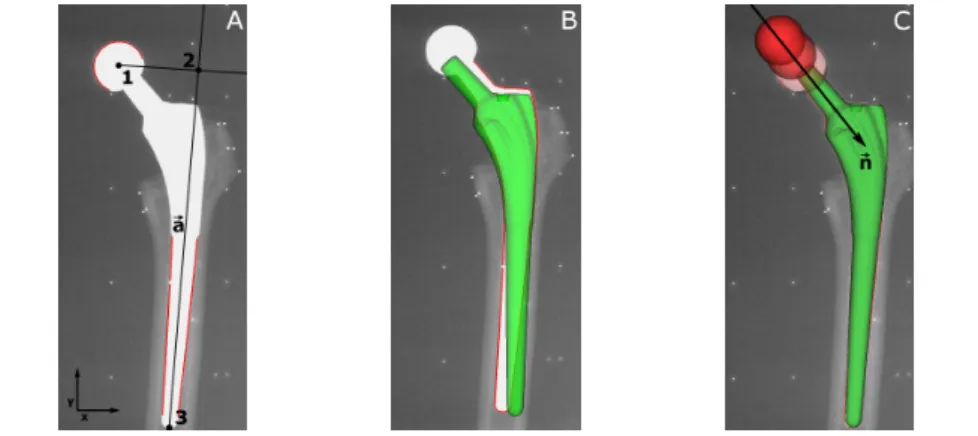
Figure 3.1: EGS-RSA: The first landmark (1) is formed by the estimation of the center of the spherical head. An axis a is estimated through the most distal part of the stem. The second landmark (2) is obtained by projecting landmark

1 onto the axis a, while the third landmark (3) is formed as the projection of the tip of the stem onto axis a. MB-RSA: The 3D surface model of the stem is used to minimize the distance between a virtually projected contour and the detected contour. CM-RSA: A combined head-stem model is used to minimize the distance between a virtually projected contour and the detected contour, while allowing the position of the spherical head to vary during the minimization.

The second landmark is obtained by projecting the first landmark, the center of the spherical head, onto this central axis.

(41)

through the focus positions and the initial guesses of the tip. The projec-tion of the 3D tip posiprojec-tion onto the central axis of the stem results in the third landmark. With three landmarks, sufficient information is available to compute the position and orientation of the prosthesis in 3D.

3.2.2 Model-based RSA

This method (MB-RSA) uses a 3D surface model of the stem. This 3D surface model is used to determine the position and orientation of the pros-thesis, by aligning it with the detected contours of the prosthesis in the image (Figure 3.1b): Contours are detected using the Canny Edge detec-tor [Canny, 1986], after which the contour parts of the stem are manually selected. To reduce the computation time, 25% of the detected contour is used for the alignment of the surface model. The alignment of the surface model is performed by calculating a contour of the virtually projected 3D surface model, followed by a calculation of the distance between this virtual contour and the actual, detected, contour. The correct pose of the surface model is then determined by searching through the six-dimensional parame-ter (position + orientation) space for an optimal pose, which minimizes the distance between the contours.

3.2.3 Combined stem-head model

(42)

Contours are detected using the Canny Edge detector [Canny, 1986], after which the correct contour parts are manually selected. Because the 3D surface model is now composed of a stem and a head, contour parts for the head are selected as well. To reduce the amount of computation time, 25% of this detected contour is used for the aligning of the surface model. Equivalent to the MB-RSA method, the alignment of the surface model is performed by calculating contours of the virtually projected combined model, followed by a calculation of the distance between this virtual contour and the actual, detected, contour. The correct pose is then determined by searching through the seven-dimensional parameter space for an optimal pose which minimizes the distance between these contours.

3.3 Experimental setup

The new method (CM-RSA) was validated in both a phantom study and on clinical data, where it is compared to MB-RSA and EGS-RSA.

3.3.1 Phantom experiment

The phantom study was performed on five prostheses (of three different hip stem designs).

• Mallory/Head size 9 and size 12 (Biomet, Inc, Warsaw, IN, USA)

• SL-Plus size 4 (Plus Orthopedics AG, Rotkreuz, Switzerland)

• Two straight Stanmore prostheses size 3 (Biomet, Inc, Warsaw, IN,

USA)

(43)

and Wedin, 1993]. For the SL-Plus prosthesis, a cup was added in which the spherical head was placed.

Eleven RSA-images were made of each prosthesis. Between exposures, the entire phantom was placed in a position and orientation mimicking the clin-ical situation. Furthermore, between exposures, the phantom was reposi-tioned manually, each time in a similar clinically relevant position, but with an overall variation of roughly 15◦ orientation. The RSA-setup consisted of two synchronized roentgen tubes at 1.5 m above the roentgen film and were directed towards the roentgen film, each one making an angle of 20◦ with the vector perpendicular to the roentgen film. Migrations between pairs of consecutive scenes were computed. I.e. the migrations were computed between the following scene-pairs: (1, 2), (2, 3), (3, 4).

3.3.2 Clinical data

In addition to the phantom experiment, the CM-RSA method was applied to clinical double-examination data. 11 double stereo roentgen-images were available for the Mallory/Head prostheses (sizes 7−14) with a metal-backed cup. For the standard Stanmore-prostheses (size 2 and size 3), eleven double images were available with a polyethylene cup. In both cases, migrations were computed between corresponding image pairs.

3.3.3 Validation

Laser-scanning (TNO Industry, Eindhoven, The Netherlands) with a spatial resolution of 0.05 mm, was used to generate reverse-engineered 3D surface models for the prostheses. The images were analyzed using Model-based RSA 3.12 (Medis specials, Leiden, The Netherlands) using standard methods for calibration and the described three methods (MB-RSA, EGS-RSA and CM-RSA) for the estimation of the position and orientation of the prosthesis.

(44)

in the (saw)bone. Therefore, the measured migration represents the mea-surement error. The mean migrations give an indication of the systematic error of the measurements, while the standard deviations give an indication of the precision of the measurements. Migrations were computed using the calibration box as the global coordinate system: the reference coordinate system is illustrated in Figure 3.1a, with the x- and y-axes in the image plane and with the z-axis perpendicular to the image plane.

Levene’s test for equality of variances was used to compare the standard deviations of the three methods.

3.4 Results

The time needed for the analysis of a pair of roentgen-images was comparable between the three methods and ranged from three to five minutes. For each method and each prosthesis, means and standard deviations for both the translational and rotational components of the measured migrations were computed. The results from the phantom-experiment and the clinical double-examinations are presented in Table 3.1.

Method Translations Rotations

x(mm) y(mm) z(mm) x(◦) y(◦) z(◦) Phantom EGS-RSA 0.02 [0.05] 0.00 [0.10] 0.00 [0.12] 0.01 [0.15] 0.01 [0.51]1 ₋₀_._{01 [0}_._09]

Mallory-Head MB-RSA −0.01 [0.05] 0.00 [0.06] 0.00 [0.13] 0.00 [0.22] 0.00 [1.01] 0.00 [0.13] (N= 22) CM-RSA −0.01 [0.05] 0.00 [0.06] 0.00 [0.09] 0.00 [0.22] 0.00 [0.67] 0.01 [0.12] Phantom SL EGS-RSA−0.02 [0.07] 0.00 [0.13] 0.01 [0.29]1 ₋₀_._{09 [0}_._34] ₋₀_._{01 [2}_._22]1 ₋₀_._{00 [0}_._20]1

SL Plus MB-RSA −0.01 [0.04] 0.01 [0.07] 0.00 [0.10] −0.04 [0.27] 0.00 [1.00] −0.00 [0.09] (N= 9) CM-RSA 0.00 [0.07] 0.01 [0.11] −0.01 [0.49]1 ₋₀_._{04 [0}_._22] ₀_._{00 [1}_._23] ₋₀_._{00 [0}_._09]

Phantom EGS-RSA 0.00 [0.04]1 ₀_._{00 [0}_._09]1 ₀_._{01 [0}_._23]1 ₀_._{01 [0}_._15] ₀_._{00 [0}_._66] ₀_._{02 [0}_._08]

Stanmore MB-RSA 0.00 [0.02] 0.00 [0.03] 0.01 [0.09] −0.02 [0.15] 0.01 [0.94] 0.04 [0.11] (N= 22) CM-RSA 0.00 [0.03]1 ₀_._{00 [0}_._02] ₀_._{00 [0}_._06] ₀_._{00 [0}_._13] ₀_._{00 [0}_._37]1 ₀_._{01 [0}_._04]1

Clinical EGS-RSA −0.02 [0.12] 0.11 [0.21] −0.12 [0.30] 0.03 [0.27] −0.41 [1.02] 0.06 [0.08] Mallory-Head MB-RSA 0.00 [0.08] −0.02 [0.11] 0.02 [0.17] 0.02 [0.22] −0.02 [0.52] 0.03 [0.10] (N= 11) CM-RSA −0.05 [0.14] −0.03 [0.19] 0.10 [0.20] 0.02 [0.20] −0.07 [0.43] 0.04 [0.09] Clinical EGS-RSA 0.01 [0.03] 0.04 [0.06] 0.01 [0.08] 0.01 [0.15] 0.12 [0.32] −0.02 [0.06] Stanmore MB-RSA 0.02 [0.05] 0.01 [0.07] 0.00 [0.08] 0.00 [0.18] 0.20 [0.24] −0.03 [0.05] (N= 11) CM-RSA 0.03 [0.06] 0.02 [0.07] −0.04 [0.11] −0.02 [0.16] 0.17 [0.20] −0.02 [0.06]

1_{Significantly different from MB-RSA}

Table 3.1: Migration results (mean [standard deviation]) for each method applied to each prosthesis.

(45)

is presented in figure 3.2. The standard deviations show that CM-RSA performed significantly better (p = 0.02) on the y-rotation than MB-RSA (0.69◦ vs. 0.96◦), while on the clinical dataset, there was no significant difference (0.41 vs 0.35). For the translation along the y-axis, there is a slight increase (from 0.05 mm to 0.06 mm) on the phantom data, while there is a significant increase (from 0.09 mm to 0.14 mm,p= 0.04) on the clinical data. EGS-RSA performs similar to MB-RSA (1.02◦ vs. 0.96◦) on the phantom data for the rotation about the longitudinal axis and significantly worse (0.10 mm vs. 0.06 mm, p <0.01) for the translation along the longitudinal axis. On the clinical data, it appeared to perform worse than MB-RSA. Its standard deviations (0.15 mm and 0.79◦) were significantly larger (p= 0.02 andp <0.01, respectively) than MB-RSA.

For the individual experiments, it can be seen that for the phantom data the mean translation errors were all below 0.1 mm, indicating small systematic errors. For the clinical experiment these values were in general slightly higher, with values below 0.12 mm.

Similarly, the mean rotation errors were mostly below 0.1◦, with some ex-ceptions: in the clinical data a mean y-rotation of 0.49◦ was measured for EGS-RSA applied to the Mallory/Head data. All three methods had a rela-tively large mean y-rotation on the clinical Stanmore data, with 0.12◦, 0.20◦ and 0.17◦ for EGS-RSA, MB-RSA and CM-RSA, respectively.

(46)

Figure 3.2: The measured Y-translations and Y-rotations for the three methods (EGS-RSA, MB-RSA and CM-RSA). On the left: The Y-translation for the phantom dataset and the clinical dataset. On the right: the Y-rotation for the phantom and clinical dataset. The boxes represent mean standard deviation.

respectively.

For each prosthesis, Levene’s test for equality of variances was used to de-termine if CM-RSA or EGS-RSA showed a significant improvement over MB-RSA. Several significant differences were found. E.g. when considering the y-rotations, EGS-RSA performed significantly better than MB-RSA on both the phantom and clinical data of the Mallory/Head, but at the same time it performed significantly worse on the phantom data for the SL-Plus. CM-RSA performed significantly better on the phantom data for the Stan-more prosthesis.

3.5 Discussion

Overall, the results from figure 3.2 demonstrate that the new CM-RSA method, using a combined stem-head model, can yield more accurate re-sults than the original MB-RSA method with a surface model of the stem only.

(47)

EGS-RSA on the phantom data of the Mallory/Head prosthesis, EGS-RSA performs very well, with a factor two improvement for the standard devi-ation for the rotdevi-ation about the y-axis (from 1.01◦ for MB-RSA to 0.51◦ for EGS-RSA, p = 0.01). At the same time, it also may perform better on the phantom data of the Stanmore prosthesis (from 0.94◦ for MB-RSA to 0.66◦ for EGS-RSA). The overall worse performance of EGS-RSA with respect to MB-RSA on the phantom data can probably be explained by its poor performance on the SL-Plus prosthesis. On the phantom data of the SL-Plus, EGS-RSA performs a factor two worse (p <0.01) than MB-RSA, with a standard deviation of 2.22◦ for EGS-RSA, compared to 1.00◦ for MB-RSA. The SL-Plus stem design has a rectangular cross-section, as opposed to the curved cross-sections of the Mallory/Head and Stanmore designs. For certain stem orientations, this rectangular cross-section can make the esti-mation of the orientation troublesome. This suggests that the performance of EGS-RSA depends partially on the shape of a particular prosthesis.

In clinical practice the precision is usually worse than the precision in a controlled phantom experiment. For the Mallory/Head and the Stanmore prostheses, this is not visible in the results. The improvement of CM-RSA with respect to MB-RSA as visible in the phantom data, is not clearly present in the clinical data. For the Mallory/Head prosthesis, there is a small non-significant improvement from 0.54◦ to 0.40◦ and for the Stanmore prosthesis MB-RSA already achieves good results and CM-RSA yields only a marginal improvement over MB-RSA from 0.24◦ to 0.204◦.

(48)

Mallory/Head prosthesis.

For the discrepancy between phantom and clinical data for the Stanmore prosthesis a simpler explanation can be given. Most Stanmore prostheses in the clinical dataset were standard curved Stanmore prostheses, while the ones from the phantom experiment were straight Stanmore prostheses. The straight Stanmore prosthesis is much more symmetric around its longitu-dinal axis and will therefore result in a larger standard deviation for the rotation about that axis. As the standard curved Stanmore prosthesis is far less symmetrical and thus less sensitive for measurement error on ax-ial rotation, the addition of the spherical head will not yield a noticeable improvement in the double examinations. This is in line with the initial hypothesis that the addition of the spherical head will yield more precision, because the symmetry along the longitudinal axis is reduced.

The results for the phantom experiment with the SL-Plus prosthesis and the results for the clinical double-examination data for the Mallory/Head prosthesis demonstrate that even with a partial overlap of the head by a metal cup, CM-RSA shows smaller standard deviations (0.84 mm vs. 1.20 mm and 0.40 mm vs. 0.54 mm) for the rotation about the y-axis than MB-RSA. In clinical practice, such a cup will often be present and cause large parts of the spherical head to be occluded.

Kaptein et al. [2006] presented an analysis of the precision of the model-based approach and reported standard deviations for translations ranging from 0.03 mm to 0.21 mm and standard deviations for rotations ranging from 0.04◦ to 1.76◦, with the largest error found for rotation about the y-axis. As can be seen from Table 3.1, the results for MB-RSA presented here are similar.

The results for EGS-RSA are similar to the data presented by Kaptein et al. [Kaptein et al., 2006] with standard deviations for translations ranging from 0.07 mm to 0.14 mm and from 0.10◦ to 0.61◦ for rotations. Both results have the largest error for rotation about the y-axis.

(49)

translations [Mjöberg et al., 1986, Kärrholm, 1989, Kärrholm et al., 1994] and from 0.05◦ to 0.58◦ for rotations [Kärrholm, 1989, Börlin et al., 2002], the marker-based approach is currently considered the most accurate method for migration measurements.

The results in Table 3.1 show that CM-RSA and EGS-RSA can still have problems with measuring the rotation about the y-axis. Considering the magnitudes of the errors, the small increase in translation error is probably justified by the decrease of the error in the other directions. It can also be seen that there is indeed an increase in accuracy with CM-RSA as opposed to MB-RSA.

3.5.1 Conclusion

It was demonstrated that using a combined stem-head model, with optimisa-tion of the head posioptimisa-tion during estimaoptimisa-tion of the pose of a prosthesis, yields more precise migration measurements on the phantom data when compared to a model-based approach with surface models of the stem only. On the same phantom data was demonstrated that elementary geometrical shapes can also be a feasible method for migration measurements on some implant designs.

Overall, CM-RSA appears to be a feasible alternative to MB-RSA. As op-posed to CM-RSA and MB-RSA, EGS-RSA eliminates the need for an ac-curate (reverse engineered) surface model, but it is only applicable in cases where the shape of the implant can be described by elementary geometrical shapes.

(50)

3.5.2 Future Work

One of the reasons for adding the spherical head to the model of the pros-thesis was to show that pose estimation using a combined model is feasible. Now that this is demonstrated, the method can be applied to other mod-ular prostheses. E.g. when focusing on knee prostheses, a combined tibial stem-plateau model can be constructed and used to increase the accuracy of RSA.

3.5.3 Acknowledgement

(51)

(52)

CHAPTER

4

DETECTING FEMUR-INSERT COLLISIONS TO IMPROVE PRECISION OF FLUOROSCOPIC KNEE ARTHROPLASTY ANALYSIS

A.H. Prins1_{, B.L. Kaptein}1_{, B.C. Stoel}2_{, J.H.C. Reiber}2_{, E.R. Valstar}1,3

1. Biomechanics and Imaging Group, Department of Orthopaedics, Leiden University Medical Center, The Netherlands

3.Department of Biomechanical Engineering, Faculty of Mechanical, Maritime, and Materials Engineering, Delft University of Technology, The Netherlands

(53)

Abstract

(54)

Detecting femur-insert collisions

4.1 Introduction

Fluoroscopic analysis is an important tool for assessing in vivo kinematics of knee prostheses. In a typical fluoroscopic setup, the subject performs a certain task (e.g. a step-up, a lunge-motion, etc.), while fluoroscopy is used to capture the internal motion of the prosthesis.

In general, shape matching techniques from the field of computer vision are used to align the shape of a 3D surface model of the implant with its silhouette detected in the image [Banks and Hodge, 1996, Hoff et al., 1998, Zuffi et al., 1999, Kaptein et al., 2003, Tashman and Anderst, 2003, Li et al., 2008]. A virtual contour of a 3D surface model of the prosthesis is calculated and compared with the actual contour of the silhouette, detected in the image. The difference between the virtual and actual contour is minimized using an optimization method.

In a bi-plane setup, high precision motion estimations have been reported [Tashman and Anderst, 2003, You et al., 2001, Kaptein et al., 2003, Li et al., 2008] from 0.06 mm to 0.23 mm for translations and from 0.07 to 1.2 for rotations. In a standard bi-plane setup, however, the freedom of movement for the subject is limited due to the presence of an extra X-ray tube and detector. A single-plane setup allows for sufficient freedom of movement, but it has serious effects on the precision of the shape matching: the out-of-plane precision, with values ranging from 1.4 mm to 4.0 mm, is much worse than the in-plane precision, where absolute precisions in measuring translations from 0.09 mm to 0.46 mm are reported [Banks and Hodge, 1996, Hoff et al., 1998, Mahfouz et al., 2003, Komistek et al., 2003, Kanisawa et al., 2003]. Precisions of the orientation measurement with single-plane fluoroscopy are between 0.35 and 1.3 [Banks and Hodge, 1996, Hoff et al., 1998, Mahfouz et al., 2003, Komistek et al., 2003, Kanisawa et al., 2003], which are comparable to those of bi-plane measurements.

(55)

Figure 4.1: Example demonstrating a standard fluoroscopic image with the mod-els overlaid in the poses estimation with normal MBRSA in the left image. The right image shows the displacement with the collision marked.

in the out-of-plane direction and simply use the same z-coordinate as the tibial component. Alternatively, we propose to incorporate collision detec-tion into the pose estimadetec-tion method. We investigated whether it would be feasible to improve the estimation of out-of-plane positions by preventing femur-insert collisions. It has been demonstrated previously in Roentgen Stereo-photogrammetric Analysis (RSA) how the use of Reverse Engineered (RE) models instead of Computer Aided Design (CAD) models can improve the accuracy of the pose estimation [Kaptein et al., 2003]. To assess the ef-fects of model accuracy on the out-of-plane position we investigated how the normal method and the new method are affected by the use of RE models and CAD models.

The poses were estimated in a single-plane setup by the new method, the normal model-based approach by Kaptein et al. [2003] and the method pro-posed by Banks and Hodge [1996]. The results of these three methods were compared to those from the much more accurate bi-plane setup, as a gold standard.

4.2 Methods

(56)

1. A combined model is constructed, similar to the models by Prins et al. [Prins et al., 2008];

2. A similarity measure is constructed between the combined model and the images, which takes collisions into account;

3. An optimization method is then used to determine the optimal pose of each component in the combined model.

1. Combined model: A combined surface model [Prins et al., 2008] is constructed from surface models of the femoral and tibial components and the polyethylene insert, with a total of twelve parameters. In this combined model, six parameters are used to control the position and orientation of the femoral component and the remaining six parameters control the position and orientation of the tibial component. Similar to a real implant, the insert in this combined model is placed in a fixed position with respect to the tibial component.

2. Similarity measure: An overall similarity measure is constructed com-posed of a contour measure and a collision measure. The contour mea-sure indicates the difference between a virtual projection of the model and contours detected in the image, while the collision measure indi-cates the extent of an intersection between the femoral component and the polyethylene insert.

• Contour measure: Similarly to the normal model-based pose

esti-mation method [Kaptein et al., 2003], contours are detected using a Canny edge detector [Canny, 1986] and the parts corresponding to the femoral and tibial components are selected manually. For each component the average distance is calculated between points on the actual contour detected in the image, and the projected contour of the surface model. This results in two differences,Df

and Dt, for the femoral and tibial component, respectively.

• Collision measure: In addition to the two similarity measures,

(57)

Figure 4.2: Example demonstrating how medial-lateral motion of the femoral component can result in an intersection with the post of the insert. The inter-section curve is defined by the locations where the outer surfaces of the femoral component and the insert intersect.

the insert component is composed of a set of volumes. An exam-ple of such a situation is presented in Figure 4.2, with a closed curve formed by the surface that the outer surfaces of two compo-nents have in common. We use the length of this boundary-curve as an indication of the amount of collision. The sum of the lengths of these curves determines an overall collision measure,Dc, which

gives an indication for the extent of the intersection.

• Overall measure: The femoral component is prevented from in-tersecting with the insert, by using the collision measure as a penalty term. When no intersection is present (Dc= 0), there is

obviously no penalty And the overall measure is then constructed asD=Df+Dt+wDc. Pilot experiments showed thatw= 0.5

was a reasonable value for the weight of the collision in this overall measure.

(58)

• Constrained 2: The relative out-of-plane position is determined

by the two z-positions of the femoral and tibial component. The simplest approach is used, which optimizes only those two Z-position parameters, while keeping the other parameters as they were obtained during the first phase.

• Constrained 6: To give the optimizer some additional freedom to correct errors in the relative out-of-plane position and to deter-mine if it will also result in a more consistent in-plane position, all six position-parameters are optimized, whereas the orientation parameters were kept unchanged.

• Constrained 12: To correct for possible small errors in orientation and position and to determine feasibility of a full optimization, optimization on all twelve parameters (controlling pose of both components) is performed. Thus, repeating the entire optimiza-tion process based on the initial pose of the first step, but now with additional collision prevention.

4.3 Experimental setup

In a bi-plane flat-panel fluoroscopic setup (Toshiba Infinix-NB: Toshiba, Zoetermeer, The Netherlands), two C-arms were used with the image de-tectors perpendicular to each other. Using a small calibration box, with a known configuration of embedded markers, the relative X-ray focus positions were calculated [Koning et al., 2007].

(59)

was performed.

To evaluate the effects of model accuracy in a single plane fluoroscopic setup, the analysis was performed with RE and CAD models. The RE models were made from the very same components as were used in the experiment, resulting in the best possible models with respect to accuracy. The following methods were considered:

Reference: As a gold standard measurement, the bi-plane data (from both image detectors) was analyzed with normal model-based pose estima-tion [Kaptein et al., 2003].

Normal: Normal model-based pose estimation was applied to the single-plane data [Kaptein et al., 2003].

Banks: The results from Normal; followed by a correction to zero of the relative pose of the femoral component [Banks and Hodge, 1996].

Constrained 2: The results from Normal; followed by a correction with optimization of the two z-positions of the components in a combined model with collision detection.

Constrained 6: The results from Normal; followed by a correction with optimization of the six position-parameters of the components in a combined model with collision detection.

Constrained 12: The results from Normal; followed by a correction with optimization of all twelve parameters of the components in a combined model with collision detection.

(60)

4.4 Results

A typical result of the constrained pose estimation is presented in Figure 4.3. As measures of accuracy and precision, the mean and standard devia-tion of the differences in posidevia-tion and in orientadevia-tion between the methods and the Reference method are presented in Figure 4.4 for the RE models and in Figure 4.5 for the CAD models. Bland-Altman plots [Martin Bland and Altman, 1986] for the relative z-position were used to present the corre-spondence for the out-of-plane direction (see Figure 4.6). As expected, the Normal method showed a large systematic error (2.0mm for RE models and 5.3mm for CAD models) in the out-of-plane direction.

Figure 4.3: Example demonstrating a standard fluoroscopic image with the mod-els overlaid in the poses estimation with constrained MBRSA in the left image. Note that this image is virtually identical to the left image in Figure 4.1. The right image shows the corrected displacement without visible collisions.

With CAD models, the correction of the relative z-position of the femoral component (Banks) reduced this large systematic error significantly (p¡0.001) to 1.1mm, without change in its standard deviation. With RE models, how-ever, it introduced a systematic error of -2.6mm. This error of Banks method is represented as a straight line in Figure 4.6, because it is the direct result of a difference between the actual measurement by the Reference method and the relative z-position of zero imposed by Banks et al.

(61)

With CAD models, the use of only the two z-position parameters (Con-strained 2) goes at the expense of a significant increase in the standard deviation (from 0.7 – 2.0 mm, p = 0.005). With RE models, the standard deviation for the out-of-plane error improved as well (from 0.7 – 0.3 mm, p <0.001).

The other two constrained methods showed significantly decreased standard deviations for the relative out-of-plane position: Constrained 12 improved to 0.1 mm (p < 0.001) with RE models and to 0.5 mm (p = 0.010) with CAD models. Constrained 6 improved to 0.1 mm (p < 0.001) and to 0.4 mm (p <0.001), for RE and CAD models, respectively.

Figure 4.4: Mean (left) and standard-deviations (right) of the differences with RE models from the stereo measurement for the position and orientation of the femoral component relative to the tibial component.

Figure 4.5: Mean (left) and standard-deviations (right) of the differences with CAD models from the stereo measurement for the 24 position and orientation of the femoral component relative to the tibial component.

(62)

a difference with CAD models: it appeared that Constrained 6 achieved lower mean error and standard deviation for the Z-position at the cost of larger errors for the X- and Y-position. The error in X-position changed from −0.1±0.1 mm to 0.1±0.4 mm and for the Y-position it changed from 0.1±0.1 mm to 0.4±0.6 mm. The Constrained 12 method on the other hand showed only significantly smaller mean errors for the X- and Y-positions and slightly larger standard deviations. The largest errors with the Constrained 12 method manifested themselves in the orientations, with significant increases for means and standard deviations of the errors of all orientations. The error in the Y-rotation of 1.2◦ ±1.0◦ in particular was significantly worse (p <0.001 for mean and standard deviations) than the Normal method.

Figure 4.6: Bland-Altman plots for the out-of-plane position of the femoral com-ponent, relative to the tibial component. The left plot demonstrates the results with RE models and the right plot those with CAD models. The average with the bi-plane reference measurement is presented on the x-axis with the differences with respect to the reference measurement on the y-axis.

4.5 Discussion

For the out-of-plane Z-position, there is clearly an improvement in accuracy and precision using collision detection in single plane fluoroscopy. With RE models, this is without significant effect on the other parameters, while the results with CAD models demonstrate that improvements are still possible, but at the expense of a decreased precision for the other parameters.

(63)

a large relative displacement of the femoral component of 5.3 mm out-of-plane would imply a femur-insert intersection as demonstrated in Figures 4.1 and 4.2. This large difference is due to the errors in absolute positions of the two components:

The absolute femoral position is biased towards the X-ray focus (3mm with CAD and 0.5mm with RE), while the tibial position is biased towards the image detector (-2mm with CAD and -1.5mm with RE). This opposite shift increases the overall difference out-of-plane between the two components. A systematic error of 5.3 mm with CAD models is much higher than has been reported before [Banks and Hodge, 1996, Mahfouz et al., 2003]. This large error is likely caused by high sensitivity of the estimation of the out-of-plane position to model inaccuracies: when the surface model is slightly smaller than the actual implant the estimate of the out-of-plane position will be further away from the image plane and this can easily be up to a few millimeters.

The large differences in results between CAD and RE models clearly demon-strate that the use of accurate models is very important in a single-plane setup. Note that in clinical practice, the RE models are not made from the very same component as implanted in the patient. So this paper shows the best and the worst case scenario.

Fixing the relative out-of-plane position as applied by Banks improves the accuracy to 1.2 mm for CAD models, but without an improvement of the precision. An additional consequence of fixing the out-of-plane position of the femoral component is that any information on that parameter during a task is lost. We believe this is what occurs with the RE models, where the correction by Banks shows much larger errors (-2.4mm ? 1.4mm).