COMPUTATIONAL TOOLS FOR CLASSIFYING AND VISUALIZING RNA STRUCTURE CHANGE IN HIGH-THROUGHPUT EXPERIMENTAL DATA
Chanin Tolson Woods
A dissertation submitted to the faculty at the University of North Carolina at Chapel Hill in partial fulfillment of the requirements for the degree of Doctor of Philosophy in the
Bioinformatics and Computational Biology Curriculum in the School of Medicine.
Chapel Hill 2017
© 2017
ABSTRACT
Chanin Tolson Woods: Computational tools for classifying and visualizing RNA structure change in high-throughput experimental data
(Under the direction of Alain Laederach)
Mutations (or Single Nucleotide Variants) in folded RiboNucleic Acid (RNA) structures that cause local or global conformational change are riboSNitches. Predicting riboSNitches is challenging, as it requires making two, albeit related, structure predictions. The data most often used to experimentally validate riboSNitch predictions is Selective 2’ Hydroxyl Acylation by Primer Extension, or SHAPE. Experimentally establishing a riboSNitch requires the quantitative comparison of two SHAPE traces: wild-type (WT) and mutant. Historically, SHAPE data was collected on electropherograms and change in structure was evaluated by “gel gazing.” SHAPE data is now routinely collected with next generation sequencing and/or capillary sequencers. We aim to establish a classifier capable of simulating human “gazing” by identifying features of the SHAPE profile that human experts agree “looks” like a riboSNitch.
To my parents, James and Pollie, who from my earliest days pushed me to always do the “hard thing”, and encouraged me whenever I came up short. Those lessons stayed with me and without
them I would not be writing this dissertation.
To my husband, Makieal, who tries to remind me to laugh, to take naps, to eat the extra fish stick and to let it all go. You have been my sanity in an otherwise insane process. I love you.
ACKNOWLEDGEMENTS
There are many people who have helped me navigate my time in graduate school. The BBSP program staff has been vital in providing me with resources to succeed during my year in the umbrella program and long after. I especially want to acknowledge Jessica Harrell and Ashalla Freeman for helping me through a particularly rough patch. I also want to thank Olga Gonzalez-Lopez for mentoring me during this time. The BCB curriculum director, Tim Elston, and program administrators, John Cornett and Cara Marlow, have helped me to tailor the program’s resources to best supplement my learning. My committee members have been assets in my development as a graduate student. They held me to a high standard and pushed me to understand the broader context of my work, particularly my committee chair Terry Furey. And David Gotz has provided guidance on data visualization and encouraged me to iterate over my design. I would like to acknowledge our collaborators Nikolay Dokholyan and Benfeard Williams for providing me with their 3D modeling expertise.
TABLE OF CONTENTS
LIST OF FIGURES ... xii
LIST OF ABBREVIATIONS ... xiv
CHAPTER 1: INTRODUCTION ... 1
1.1 Messenger RNA ... 1
1.2 RNA Structure ... 5
1.3 RNA Structure Probing ... 7
1.4 RNA Structure Prediction ... 11
1.5 Boltzmann Suboptimal Sampling ... 16
1.6 Machine learning in classification ... 18
1.7 Random Forest and Classification of RNA Structure Change ... 19
1.8 RNA Structure Visualization ... 23
CHAPTER 2: CLASSIFICATION OF RNA STRUCTURE ... 28
2.1 Introduction ... 28
2.2 Methods... 30
2.2.1 Data Set ... 30
2.2.2 Data normalization and noise reduction ... 31
2.2.3 Human expert evaluations ... 31
2.2.5 classSNitch package ... 33
2.2.6 WT SHAPE improved SNPfold ... 34
2.3 Results ... 34
2.3.1 The “obvious” riboSNitch ... 34
2.3.2 Human consensus on local and global structure change ... 37
2.3.3 Automated classification of mutation induced structure change ... 45
2.3.4 classSNitch analysis of experimental structure change ... 48
2.3.5 WT SHAPE informed riboSNitch detection ... 50
2.4 Discussion ... 52
2.5 Methods Supplementary ... 57
2.6 Supplementary Materials ... 64
CHAPTER 3: VISUALIZATION OF THE RNA SUBOPTIMAL ENSEMBLE ... 84
3.1 Introduction ... 84
3.2 Materials and Methods ... 89
3.2.1 Generating structures for the map of conformational space ... 91
3.2.2 Projection of the map of conformational space ... 92
3.2.3. EnsembleRNA package ... 93
3.2.4. In vitro SHAPE treatment ... 93
3.2.5. In vivo SHAPE treatment ... 94
3.2.6. SHAPE data collection and analysis ... 94
3.2.9. RNA Dynamics ... 96
3.3 Results ... 97
3.3.1 Generating a robust 2-dimensional representation of an RNA ensemble ... 97
3.3.2. Detecting RNA structure change induced by ligand binding ... 98
3.3.3. Observing regional structure differences in vitro and in vivo ... 101
3.4 Discussion ... 108
3.5 Supplementary Materials ... 113
CHAPTER 4: CONCLUSION ... 122
4.1 Important Findings ... 124
4.2 Approach Weaknesses ... 125
4.3 Future directions ... 127
LIST OF TABLES
Table 2.1 Expert evaluation summary ... 38
Table 2.2 Features used to quantify differences between WT and mutant traces ... 43
Table 2.3 RNAs for use in analysis ... 76
Table 2.4 Formula and descriptions for features describing SHAPE trace pairs ... 77
Table 2.5 Algorithm selection ... 78
Table 2.6 Breakdown of mutations for the mutate-and-map data set ... 79
Table 2.7 Formula symbols ... 80
Table 2.8 Validation Traces ... 81
Table 2.9 Feature Statistics ... 82
LIST OF FIGURES
Figure 1.1. SHAPE-MaP Methodology. ... 10
Figure 1.2. Nearest-neighbor model for a stem loop. ... 13
Figure 1.3. Dynamic programming methodology. ... 15
Figure 1.4 A random forest model decision tree ... 21
Figure 1.5 Current methods for RNA structure visualization. ... 26
Figure 2.1 Structure change patterns in SHAPE trace data for glycine riboswitch aptamers ... 36
Figure 2.2 Expert evaluation of RNA structure change in SHAPE data ... 40
Figure 2.3 classSNitch performance ... 47
Figure 2.4 Fraction of disruption for individual RNAs ... 51
Figure 2.5 Improving the performance of structure change prediction algorithms ... 53
Figure 2.6 Differences between top performing algorithms ... 64
Figure 2.7 Robustness to noise ... 65
Figure 2.8 Feature descriptions ... 66
Figure 2.9 Dynamic time warping feature ... 68
Figure 2.10 Feature selection ... 70
Figure 2.11 Dynamic time warping versus eSDC ... 71
Figure 2.12 Probability of disruption for 16S Four-Way Junction ... 73
Figure 2.13 Improving the performance of structure change prediction algorithms ... 74
Figure 3.1. The conformational states of the vibrio vulnificus add adenine riboswitch. ... 85
Figure 3.2. Building the map of conformational space. ... 89
Figure 3.3 Visualization of the vibrio vulnificus add adenine riboswitch. ... 100
Figure 3.5. Ensemble visualization for in vitro and in vivo human β-actin mRNA. ... 107
Figure 3.6. RNA structure abstraction and nestedness. ... 113
Figure 3.7. Projection of the reference RNA. ... 114
Figure 3.8. Comparison of similar in vitro and in vivo structure for the β-actin mRNA. ... 115
Figure 3.9. Similar in vitro and in vivo ensembles for human β-actin mRNA. ... 117
Figure 3.10. Comparison of different in vitro and in vivo structure for the β-actin mRNA. ... 118
LIST OF ABBREVIATIONS RNA DNA mRNA poly(A) UTR tRNA eRF1 PARS FTL IRE IREBP NMR SHAPE SHAPE-MaP cDNA MFE PCA MDS RiboNucleic Acid Deoxyribonucleic Acid Messenger Ribonucleic Acid Poly Adenine
Untranslated Region Transfer Ribonucleic Acid
Eukaryotic Translation Termination Factor 1 Parallel Analysis of RNA Structure
Ferritin Light Chain Iron Response Element
Iron Response Element Binding Protein Nuclear Magnetic Resonance
Selective 2’-Hydroxyl Acylation by Primer Extension
Selective 2’-Hydroxyl Acylation by Primer Extension & Mutational Profiling Complementary Deoxyribonucleic Acid
Minimum Free Energy
CHAPTER 1: INTRODUCTION
Machine learning has become an integral part of our lives. These algorithms help us to do everything from shopping to communicating to working out. Every technological device we own, our computers, our phones, even our watches are involved in forming a representation of our lives in data. In the biomedical sector, these algorithms are revolutionizing healthcare diagnostics. These types of tools are being used to predict spiking blood pressure levels in
intensive care patients and to monitor a patient’s neurological condition in real-time (Kohn et al., 2014). And with the emergence of high-throughput technology, we can leverage these learning algorithms to glean insight into hidden patterns and complex systems found in large, complex biological data sets as well. Machine learning algorithms are being applied to topics in biology as varied as protein structure classification and estimating bias in microarray data (Qi, 2012). In this work, we describe the development of two computational tools that help analyze the role of RNA structure in human health.
1.1 Messenger RNA
Ribonucleic acid (RNA) is involved in many different functions in a cell, such as
to the 5’ end of the DNA template strand, the RNA polymerase unwinds the DNA and transcribes the complementary RNA strand (Lee and Young, 2000). The growth of the RNA strand is called elongation (Lee and Young, 2000).
reaches the RNA polymerase and detaches it from the DNA (Dever and Green, 2012). An adenine tail is added to the newly formed precursor mRNA (pre-mRNA) (Shatkin and Manley, 2000). This poly(A) tail is added to the 3’ end of the pre-mRNA. Polyadenylation can play a role in nuclear export and stability, but is particularly important in degradation (Shatkin and Manley, 2000). Once the poly(A) tail has been added, the now mature mRNA can be exported from the nucleus to the cytoplasm through nuclear pore complexes (Strambio-De-Castillia et al., 2010).
change occurs in the ribosome and if the anticodon sequence of the tRNA is not complementary to the three mRNA nucleotides at that position, particularly the first two positions, the tRNA will be ejected from the site (Yonath, 2010). Once a complementary tRNA has entered the A-site a peptide bond will be formed between the amino acid and the growing polypeptide chain (Yonath, 2010). The RNA portion of the ribosome catalyzes this reaction (Yonath, 2010). The ribosome then moves the tRNA in the A-site to the P-site, and the P-site tRNA to the E-site through a ratcheting motion (Dever and Green, 2012). The tRNA is then able to exit the ribosome from the E-site (Dever and Green, 2012). The growing polypeptide chain exists the ribosome through the ribosomal tunnel (Yonath, 2010). The tunnel is involved in ensuring that the protein properly folds once it has exited the ribosome (Yonath, 2010). When the stop codon is reached on the mRNA, eukaryotic translation termination factor 1 (eRF1) releases the newly formed protein from the ribosome and the two subunits dissociate (Dever and Green, 2012). The ribosome subunits can then be recycled for use on another mRNA (Dever and Green, 2012). It is also important to note that a single mRNA can have many ribosomes attached at once (Dever and Green, 2012).
RNA performs many functions in a cell and key to all of these functions is its structure. For mRNA, structure can regulate gene expression during translation initiation and elongation. Structure in the coding region can also allow for proper folding of proteins. Variants or
1.2 RNA Structure
A single-stranded RNA can fold to adopt specific conformations that are key to the functions it performs in a cell (Weeks, 2010). Over a millisecond timeframe, RNA secondary structure develops from base-pair interactions (Weeks, 2010). During the second and minute timeframe an RNA can form long-range tertiary interactions further increasing an RNAs stability (Weeks, 2010). The structure of RNA is dynamic, which may be important for function, like in the case of riboswitches that form at least two different structures (Lemay et al., 2009; Lemay et al., 2006; Lipert et al., 2007; Tucker and Breaker, 2005). Riboswitches are RNAs found in the 5’ untranslated region of an mRNA that regulate gene expression (Lemay et al., 2009; Lemay et al., 2006; Lipert et al., 2007; Tucker and Breaker, 2005). These riboswitches bind a ligand that induces a conformational change that either promotes or inhibits translation of that mRNA (Lemay et al., 2009; Lemay et al., 2006; Lipert et al., 2007; Tucker and Breaker, 2005). Another example of RNA structure playing an important role in function is gene regulation by
microRNAs, where double stranded regions are precursors for Dicer recognition to further process the microRNAs for use in the RISC complex (Mortimer et al., 2014; Wilson and Doudna, 2013).
RNA structure also plays a role in translational control in mRNAs (Mortimer et al., 2014). Structuredness in the 5’ untranslated region of an mRNA, particularly around the
intermediates required for proper folding (Komar, 2009; Mortimer et al., 2014). Structuredness in the coding region of an RNA has also been linked to increased translational efficiency (Kertesz et al., 2010; Li et al., 2012; Mortimer et al., 2014). Increased structuredness in the 3’ untranslated region of mRNAs can help localize them to the correct location in the cell (Kertesz et al., 2010; Mortimer et al., 2014). Structured 3’ untranslated regions of an mRNA can lead to longer half-lives, with less flexible 3’ ends being less targeted by the exosome complex for degradation (Wan et al., 2012).
It is important to note that while some ribonucleic acid (RNA) molecules have evolved to adopt a single conformation, a majority of RNAs are thought to adopt multiple conformations (Matthews, 2006). RNA molecules may exist in multiple conformations in order to perform a function, such as promoting or inhibiting expression of an associated gene (Lemay et al., 2009; Lemay et al., 2006; Lipert et al., 2007; Tucker and Breaker, 2005). In order to perform these functions there must be several energetically similar and easily accessible structures that RNA molecules can form (Matthews, 2006). The possible structures that RNA may take in a cell constitute its structural ensemble (Matthews, 2006).
Structural changes in RNA may lead to a functional consequence, a phenomena referred to as a riboSNitch. RiboSNitches can be created through polymorphisms and variation in DNA that is transcribed into the RNA. A recent study compared RNA structure in a human family trio (mother, father and child) on a genome wide scale using parallel analysis of RNA structure (PARS)(Wan et al., 2014). This study identified riboSNitches in 15% of over 12,000 single nucleotide variants, and 22 unique riboSNitches associated with human phenotypes and diseases, including multiple sclerosis and asthma(Wan et al., 2014). These findings indicate that
chain (FTL) is a protein subunit that is associated with Hyperferritienemia Cataract Syndrome, a genetic disorder that causes cataracts in infancy (Ritz et al., 2012). A mutation in the 5’
untranslated region of the mRNA for FTL contains an iron response element (IRE) that binds the iron response element binding protein (IREBP) (Ritz et al., 2012). A mutation in the 5’
untranslated region that does not directly alter the sequence of the IRE, changes the structure of the 5’ untranslated region preventing the IRE from binding to the IREBP (Ritz et al., 2012).
1.3 RNA Structure Probing
There are several methods for determining RNA structure. With X-ray crystallography and Nuclear Magnetic Resonance (NMR) secondary and tertiary structure can be determined, however, for many longer RNAs these methods cannot be used (Kubota et al., 2015). An
alternative set of methods for determining RNA structure is chemical probing (Ehresmann et al., 1987; Peattie and Gilbert, 1980). For these methods a chemical probe reagent interacts with a portion of the RNA and that interaction can be measured to give information on RNA structure (Weeks, 2010). There are base-specific reagents that form adducts with one or more RNA bases that provide information on base stacking, hydrogen bonding and the electrostatic environment adjacent to the modified base (Tijerina et al., 2007; Weeks, 2010). Alternatively, hydroxyl radicals can be generated to cleave RNA backbone giving information on solvent accessibility of the backbone (Tullius and Greenbaum, 2005; Weeks, 2010). Using reagents that are tethered to one section of an RNA that can react with distant regions, long-range tertiary interactions can be measured (Sigurdsson et al., 1995; Weeks, 2010). Some methods interact with specific
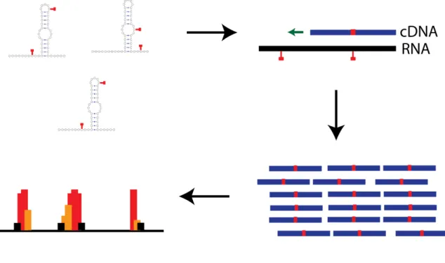
One such method that interacts with the hydroxyl of the RNA backbone is selective 2’-hydroxyl acylation analyzed by primer extension (SHAPE) (Wilkinson et al., 2006). SHAPE reagents react with the 2’hydroxyl group to form an adduct (Wilkinson et al., 2006). These reagents preferentially form adducts in more flexible regions (more likely unpaired), because these regions are more likely to adopt conformations that are favorable to reaction with the SHAPE reagent (Wilkinson et al., 2006). Radiolabeled complementary DNA is annealed to the modified RNA by reverse transcriptase (Wilkinson et al., 2006). Once an adduct is reached, the reverse transcriptase stops, leaving a complementary DNA fragment (Wilkinson et al., 2006). These fragments can then be size separated by gel electrophoresis or capillary electrophoresis (Mitra et al., 2008; Wilkinson et al., 2006). Positions with high modification, indicated by 3’ fragment ends, are more flexible positions (Wilkinson et al., 2006). Advancements to the SHAPE method have utilized high-throughput sequencing technology to measure hundreds of RNA sequences for several experiments at once (Lucks et al., 2011). Reagents have also been developed to allow for in vivo SHAPE analysis (Spitale et al., 2013).
SHAPE experiments can also be performed genome-wide using SHAPE and mutational profiling (SHAPE-MaP) (Figure 1.1) (Siegfred et al., 2014). In this method, an adduct induces a mutation that the reverse transcriptase can read through creating differences in the
Figure 1.1. SHAPE-MaP Methodology.
RNAs are modified by chemical reagents that preferentially form an adduct at the backbone 2’-hydroxyl for flexible positions (Siegfred et al., 2014). Reverse transcriptase produces
Many techniques have been developed to experimentally determine RNA structure. However, structures for every RNA are not always readily available or easily obtained. In these cases it may be useful to rely on computational methods for the prediction of RNA structure.
1.4 RNA Structure Prediction
For RNAs where an experimentally determined structure is unavailable, structure prediction may be a valuable tool in determining RNA secondary structure. RNA secondary structure can be predicted without knowing the tertiary structure, because secondary interactions are typically stronger and occur faster than tertiary interactions (Banerjee et al., 1993; Matthews et al., 1997; Woodson, 2000).
One of the first methods used for predicting RNA secondary and tertiary structure, comparative sequence analysis, compared multiple homologous sequences between organisms with shared ancestry (Gutell et al., 2002; Michel et al., 2000). Base-pairs were inferred by
determining canonical pairs that are common among the sequences (Gutell et al., 2002; Michel et al., 2000). Compensating base-pair changes further provided support for a base-pairing (Gutell et al., 2002; Michel et al., 2000). Comparative sequence analysis has been shown to be most
successful when many homologous sequences are available (Gutell et al., 2002).
two structures 𝑆! and 𝑆! is given by the ratio of these equilibrium constants. From these equations, the lowest free energy structure is the most common conformation at equilibrium (Matthews, 2006).
𝑆!" ⇌𝑆! (1)
𝐾! = !!!
!" (2)
𝐾! =e!!!!"
!(!)/!!
(3) !!
!! =
!! !! = e
(!!!"! ! !!!!"! !/!" (4)
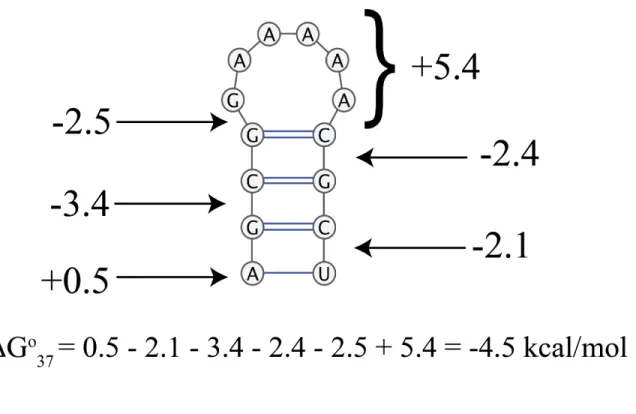
The most common method for predicting the folding free energy of a secondary structure is an empirical nearest-neighbor model (Matthews et al., 1999; Matthews et al., 2004; Xia et al., 1998). For a nearest-neighbor model, the free energy change is determined by the sequence and the most adjacent base pairs (Figure 1.2) (Matthews, 2006). The entropic contributions for the free energy change include loops and bulges, while the enthalpic contributions include base pairs and stacking (Matthews et al., 1999; Matthews et al., 2004; Xia et al., 1998). The parameters for each of these contributions have been determined experimentally (Matthews et al., 1999;
Figure 1.2. Nearest-neighbor model for a stem loop.
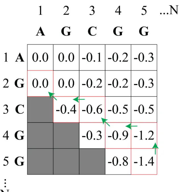
The number of secondary structures 𝑁!! grows exponentially with length 𝑁 (Eq. 5) (Giegerich et al., 2004; Matthews, 2006). To find the lowest free energy structure, dynamic programming can be implemented in order to avoid generating all possible structures (Figure 1.3) (Nussinov and Jacobson, 1980; Nussinov et al., 1978). In the fill step, the lowest free energy is determined for each sequence fragment starting with the smallest fragment and then
increasingly longer fragments (Eddy, 2004; Nussinov and Jacobson, 1980; Nussinov et al., 1978). The additive nature of the free energy calculation allows for the longer fragments to be calculated recursively (Eddy, 2004; Nussinov and Jacobson, 1980; Nussinov et al., 1978). The longest fragment is the entire sequence, so once the fill step is complete the minimum free energy for the sequence is now known (Matthews, 2006). The traceback step starts at the minimum free energy and traces backward through the fragments generated in the fill step to determine the interactions that contributed to the minimum free energy are determined (Eddy, 2004; Nussinov and Jacobson, 1980; Nussinov et al., 1978). This method guarantees the lowest free energy structure is found (Matthews, 2006).
Figure 1.3. Dynamic programming methodology.
The fill and traceback steps for dynamic programming are depicted for a model RNA fragment. The matrix shows the fill step that calculates the lowest free energy. The green arrows show the traceback step that calculates which fragments are included in the minimum free energy
RNA structure prediction can be improved with the inclusion of structure probing data (Diegan et al., 2008). An extra free energy term can be added to the nearest neighbor free energy model in order to account for the empirical information (Eq. 6) (Diegan et al., 2008). The
intercept 𝑏 represents a reward for pairing nucleotides with a low SHAPE reactivity, and the slope 𝑚 represents a penalty for pairing nucleotides with high SHAPE reactivity(Diegan et al., 2008). Parameters 𝑏and 𝑚 were determined empirically using the prediction 23S ribosomal RNA as a model RNA, where the secondary structure is known from comparative sequence analysis (Diegan et al., 2008).
Δ𝐺!!!"# 𝑖 =𝑚ln 𝑆𝐻𝐴𝑃𝐸 𝑖 +1 +𝑏 (6)
RNA structure prediction can be useful for understanding how RNA structure relates to function, particularly when a crystal structure is unavailable. While the free energy minimization using dynamic programming provides an efficient method to calculate a representative structure for an RNA, this prediction can be improved with the addition of chemical mapping data. Sampling from the entire ensemble of structures that an RNA may take in a cell, may further improve RNA secondary structure prediction, allowing for a more accurate representation of RNA structure.
1.5 Boltzmann Suboptimal Sampling
Schroeder et al., 1999). Some interactions cannot be modeled using dynamic programming (Matthews, 2006; Matthews and Turner, 2002). The assumption that the RNA is at equilibrium does not account for how folding kinetics may play a role in determining secondary structure (Heilman-Miller and Woodson, 2003; Matthews, 2006). Most importantly many RNAs, like riboswitches, have evolved to form multiple conformations, which can be important to their function (Lemay et al., 2009; Lemay et al., 2006; Lipert et al., 2007; Martin et al., 2012; Schultes and Bartel, 2000; Tucker and Breaker, 2005). All of the conformations a single RNA may sample in a cell are its structural ensemble (Matthews, 2006). For these reasons, calculation of a set of low free-energy suboptimal structures provides more information on RNA structure than just the minimum free energy structure.
The first algorithms that allowed for the prediction of suboptimal secondary structures allowed for an arbitrary starting point for the traceback step in finding the minimum free energy structure (Steger et al., 1984; Zuker, 1989). The traceback step then created a suboptimal secondary structure (Steger et al., 1984; Zuker, 1989). This method was efficient, but not all possible secondary structures could be explored (Matthews, 2006). Subsequent algorithms determined all suboptimal structures within an energy range from the minimum free energy (Williams and Tinoco, 1986; Wuchty et al., 1999). All secondary structures are calculated without redundancy in the fill step from minimum free energy calculation (Wuchty et al., 1999). The trace back step then determines all structures within a specified range of the lowest free energy structure (Wuchty et al., 1999).
Current algorithms sample suboptimal secondary structures from the Boltzmann
McCaskill, 1990). The traceback step generates base-pairs according to the partition functions for all possible sequence fragments (Ding and Lawrence, 2003; Ding and Lawrence, 1999). This creates a set of suboptimal structures that is a statistical sample of the RNA structural ensemble (Ding et al., 2005). The statistical sample is remarkably stable; a messenger RNA with over 1000 nucleotides a sample size of 1000 structures is sufficient to produce nearly the same base pairing probabilities for each run (Ding et al., 2006).
With the ability to create a statistical ensemble of RNA structures, we can more
accurately identify structural elements that are playing a role in an RNAs function (Ding et al., 2006; Ritz et al., 2012). We can also better determine how variants contribute to differences in RNA structure and how that potentially leads to differences in phenotype.
With the advent of new technologies, information on RNA structure can be gathered on a genome-wide scale. However, this large amount of data can be difficult to analyze. This
difficulty particularly exists in identifying structure change in RNAs caused by variants or polymorphisms. Algorithms in the machine learning field have been developed to address the problem of finding patterns in large data sets, and can be utilized to address this problem.
1.6 Machine learning in classification
There are three subgroups of machine learning techniques: unsupervised learning,
supervised learning, and semi-supervised learning (Hua et al., 2009; Libbrecht and Noble, 2015). Unsupervised learning finds hidden structure in unlabeled data (Raychaudhuri et al., 2009). Examples of unsupervised learning algorithms include clustering and principal component analysis (Ding et al., 2006; Raychaudhuri et al., 2009). The semi-supervised learning uses an incomplete training set for learning, because the use of even small amounts of labeled data improves the accuracy of learning (Libbrecht and Noble, 2015).
Supervised learning infers function from labeled data (Libbrecht and Noble, 2015). This subgroup includes two categories: classification, which predicts categories and regression that allows the prediction of values (Liaw and Weiner, 2002; Libbrecht and Noble, 2015). Both of these infer function from a set of known examples, and predict the function for future samples (Liaw and Weiner, 2002).
Currently, many supervised learning techniques exist that can be utilized for
classification of the change in RNA structure. One classifier that can classify RNA structure change is random forest. Such a classifier would be built on a set of features that characterize RNA structure change in chemical mapping data. A set of labeled samples would be required for use in random forest supervised learning.
1.7 Random Forest and Classification of RNA Structure Change
2010). Inputs for random forest consist of a set of N samples characterized by a set of M features. Each of these samples has a label or value (Figure 1.4A) (Breiman, 2001; Liaw and Weiner, 2002).
The random forest technique forms decision trees, which group the samples into different nodes according to the feature being measuring (Figure 1.4B) (Breiman, 2001; Chen et al., 2011). The root node is the feature that includes all of the samples (Liaw and Weiner, 2002). The features of the samples using random forest are selected at random to split the node (Liaw and Weiner, 2002). If multiple features are selected, a linear combination of the features will be used (Liaw and Weiner, 2002). The tree grows by choosing the best split based on the selected
features and breaking the samples into two new nodes (Liaw and Weiner, 2002). A node that can no longer be split, is called a leaf node, because all samples are identical or the node only
Figure 1.4 A random forest model decision tree
The importance of individual features in building a random forest classifier can be determined using the Gini importance or the permutation importance (Breiman, 2001). Gini importance calculates the average node purity or how mixed the labels are for each node (Breiman, 2001). This measure is sensitive to categorical data features with more variables (Breiman, 2001). The permutation importance determines how much the prediction accuracy decreases when a variable is removed, which is sensitive to differences in scale between features (Breiman, 2001). The fraction of trees where two elements are located in the same leaf node gives a proximity measure (Breiman, 2001). The proximity measure can be used to create a similarity matrix.
A random forest classifier produces the best error rate when the correlation between trees is low and the strength or accuracy of each tree is high (Breiman, 2001). The performance of a classifier can be improved by reducing the number of features selected to split each node (Breiman, 2001). A large number of trees is required for stable estimates (Breiman, 2001). For an unbalanced population, where one class has many more samples, the class with more samples can be under-sampled to produce better error rates (Chen et al., 2004). An alternative is
increasing the percentage of tree votes required to determine the class with more samples (Chen et al., 2004).
Random forest is widely used for several reasons; (1) the classifier is efficient on large data sets, because it is easily parallelized, (2) the generalized error rate is unbiased so there is no need for cross-validation, and (3) the method is non-parametric, so there is no assumption about the underlying population distribution (Breiman, 2001; Touw et al., 2013). Random forest performs well with many features and few cases or with few features and many cases for
there are several drawbacks. Individual trees are not useful, making the interpretation of the forest more difficult (Breiman, 2001; Touw et al., 2013). Correlated features are problematic and especially for determining feature importance (Breiman, 2001; Touw et al., 2013). The
generalization error has an upper bound, but it is still possible that the error rate for a training set is much better than the error rate for a test set (Breiman, 2001; Touw et al., 2013).
Random forest can be a useful tool in identifying structure change in chemical mapping data. Once differences in RNA structure have been identified, it is important to determine which structural elements are changing and how these relate to function. Secondary and tertiary
structural information for an RNA can be experimentally determined by techniques such as x-ray crystallography (Holbrook and Kim, 1997). However, structures resolved using such techniques are not always available. Our goal is to use computational prediction as a valuable alternative to determine how changes in RNA affects their structure.
1.8 RNA Structure Visualization
One way that we can utilize algorithms that statistically sample an RNA structural ensemble is to ompare the predicted ensembles using data visualization techniques. Data visualization is used for two purposes: data analysis and communication (Few). Visualization can be a powerful tool in identifying important structural elements in an RNA and comparing how these elements differ between variants (Ding et al., 2005; Ritz et al., 2012). RNA structure visualization also enables scientists to effectively communicate how differences in RNA
structure may affect phenotype (Ritz et al., 2012).
Zuker and Stiegler, 1981). These single structure representatives have been shown to inadequately describe RNA molecules, as they exist in an ensemble (Ding et al., 2006;
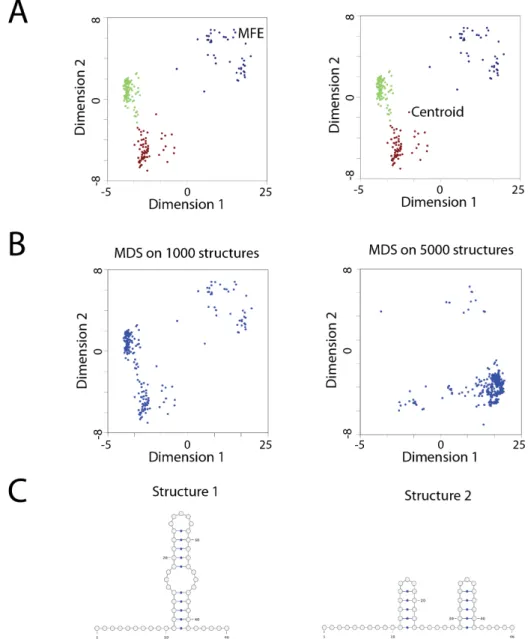
Matthews, 2006). The MFE representation assumes that at equilibrium an RNA molecule folds into a unique lowest energy state (Ding et al., 2005; Matthews et al., 1999; Zuker and Stiegler, 1981). However, the MFE structure is not always the most common structure in an ensemble (Ding et al., 2005; Ding et al., 2006). The ensemble centroid structure is the structure with the minimum base-pair distance to all other structures in the ensemble(Ding et al., 2005; Ding et al., 2006). This representation is a more accurate representation of an RNA structural ensemble, but does not account for different clusters of structures (Ding et al., 2005; Ding et al., 2006). In some cases a single structure representation is not sufficient to describe an ensemble of RNA structures (Figure 1.5A).
the smallest residual sum of squares when compared to the original distance matrix (Abdi, 2007; Torgerson, 1952). Non-metric MDS also optimizes the data point configuration but instead preserves the order of the data points not their distances (Abdi, 2007; Torgerson, 1952). This algorithm is similar to metric MDS except an additional step before optimization occurs where isotonic regression is used to relate the distance matrix to the lower dimensional projection (Abdi, 2007; Torgerson, 1952). The positioning between the structures is well maintained in all three MDS algorithms. However, new structures cannot be projected onto the space without recalculating the eigenvectors, which could greatly change the visualization (Abdi, 2007). The lack of a consistent space for projection of structures would make the addition of new structures or the comparison between structural ensembles difficult (Figure 1.5B).
𝑆𝑡𝑟𝑒𝑠𝑠= (!!"! !!!!! )!
!!"!
!" (7)
Figure 1.5 Current methods for RNA structure visualization.
CHAPTER 2: CLASSIFICATION OF RNA STRUCTURE1
2.1 Introduction
A persistent challenge in the field of structural biology is accurately predicting the
conformational and ultimately functional consequences of a mutation on a protein or nucleic acid (Chauhan and Woodson, 2008; Cheng et al., 2005; Churkin et al., 2011; Russell et al., 2002). For both nucleic acids and proteins, accurately predicting the extent of disruption is generally more challenging than predicting the entire structure (Miao et al., 2015; Waldispuhl and Reinharz, 2015; Wan et al., 2014). Indeed it requires making two, albeit related structure predictions. The data most often used in conjunction with RiboNucleic Acid (RNA) structure prediction algorithms are chemical and enzymatic probing experiments (Corley et al., 2015; Ritz et al., 2012; Solem et al., 2015). These experiments, in particular Selective 2’ Hydroxyl
Acylation by Primer Extension (SHAPE) provide nucleotide resolution structural information and are exquisitely sensitive to structure change (Cruz et al., 2012; Kutchko et al., 2015; Rice et al., 2014; Siegfried et al., 2014). Recent technological advances enable this data to be collected with unprecedented throughput (Siegfried et al., 2014); traditionally this data was carefully
human curated to ensure accuracy, which is simply not possible in the genomic context (Ritz et al., 2012; Rocca-Serra et al., 2011; Sansone et al., 2012).
Chemical and enzymatic probing techniques have long been used in structural, kinetic and thermodynamic characterizations of nucleic acids (Brenowitz et al., 1986; Brenowitz et al., 1986; Deras et al., 2000; Sclavi et al., 1997). Until the advent of capillary sequencing and more recently next generation sequencing, the experiments were carried out using traditional gel electrophoresis (Brenowitz et al., 1986; Brenowitz et al., 1986; Petri and Brenowitz, 1997). Although informatics tools were developed to rapidly quantify these complex electropherograms, most structural insight was still gleaned by “gel gazing;” for an effect to be robust the scientist had to be able to visualize it (Das et al., 2008; Das et al., 2005; Russell et al., 2002; Takamoto et al., 2004). With high-throughput probing experiments rapidly becoming the norm, it is
impossible to systematically visualize all the data.
structural change is significant. In particular, the distinction between a local structural change affecting several residues and a global structure change affecting a majority of residues.
Human ability to visually detect patterns in data is exceptional; even in the field of RNA structure, humans readily design better RNA folds than purely automated programs (Lee et al., 2014; Rowles, 2013; Treuille and Das, 2014). Interestingly, with enough examples machines can then learn the rules used by humans to make these designs (Lee et al., 2014). In this manuscript, we aim to automate some of the human skills associated with “gel gazing” and apply these to the problem of identifying riboSNitches from high-throughput SHAPE data. We are particularly interested in understanding how humans interpret SHAPE data and what features of the signal they use to classify structure change. We are also interested in determining whether there is a consensus among users of SHAPE data as to what constitutes a small or large change in RNA structure. We therefore created a platform for easily visualizing SHAPE traces and asked experts in the field to classify traces and structures. As will be shown below, there is surprising
agreement in human appreciation of the data and from these classifications we are able to
identify novel metrics that reproduce the manual classifications. We are therefore able to report a structural classification scheme that quantitatively reproduces the process of “gel gazing.” Our classifier allows us to simulate human eyes on high-throughput data sets and identify important differences in specific RNAs’ sensitivity to mutation.
2.2 Methods
2.2.1 Data Set
al., 2011). These 17 RNA database entries had a total of 2019 WT and single-point mutant trace pairs (Table 2.3). Of these trace pairs, 200 pairs were chosen for manual evaluation by 14 experts. Due to incomplete survey results we were able to obtain a majority consensus from at least 14 experts on 167 of the pairs.
2.2.2 Data normalization and noise reduction
Each WT trace was normalized to a mean reactivity of 1.5. A multiplier was used to normalize the respective mutant trace. The multiplier was chosen that minimized the difference between the WT and mutant traces. We reduced noise by setting mutant SHAPE values equal to the WT value, if both reactivities were outliers as defined by (Karabiber et al., 2013). To remove end effects, 8% of the data was trimmed from the 5’ and 3’ ends. Normalization and noise reduction are further explained in Methods Supplementary, Subsection 2.5.2.2.
2.2.3 Human expert evaluations
Therefore, it is useful to consider secondary structure in structure change prediction, but the true secondary structure for an RNA is difficult to obtain experimentally. To address this we
compared the expert classification to secondary structure prediction guided by SHAPE data. It is important to note that using predicted secondary structures in lieu of experimental structures is imperfect and likely increases the perceived secondary structure classification error by the experts. The experts did occasionally classify local changers in predicted secondary structure as global changers. However, the experts rarely classified global changers in secondary structure as local changers. (Table 2.10). Experts were filtered using a set of questions that gauged their familiarity with the biological sciences, RNA, RNA structure and SHAPE experiments. We identified 14 respondents in our survey results who self-identified as experts.
2.2.4 Feature and algorithm selection
Twenty-three features were initially used to quantify WT and mutant SHAPE trace differences and are reported in Table 2.2 and Table 2.4. These features rely solely on the
next best performing algorithms, Multilayer Perceptron and Kstar. This is particularly true for WT/mutant pairs with minimal differences in pattern, but sizeable differences in magnitude such as the G55U mutation in the 16S four-way junction, which we illustrate in Figure 2.6. KStar and Multilayer Perceptron mislabel the pair as a local changer, while Random Forest correctly identified the pair as a non-changer in agreement with the majority vote of experts. Although these minor differences in classification do not indicate that random forest is statistically better than Kstar and Multilayer Perceptron, the correct classification by random forest on these particularly difficult comparisons led us to choose it for implementation in the classSNitch approach. We built a random forest classifier on the set of 167 trace pairs using the
randomForest R package with 5001 trees and default settings (Breiman, 2001; Liaw and Wiener, 2002). The random forest classifier was used to predict the classes for the entire set of 2019 normalized and noise reduced WT/mutant trace pairs. Feature selection, algorithm selection, and model building are further explained in Methods Supplementary, Subsection 2.5.2.4. The
model’s robustness to noise was tested using both simulated noise and repeated experiments (Figure 2.7).
2.2.5 classSNitch package
An R package was created for the identification of RNA structure change in large amounts of SHAPE data. The package includes methods for normalization, noise reduction, and calculating features. Feature calculations include pattern change, dynamic time warping, change contiguousness, Pearson correlation, Euclidean norm, change variance, eSDC and change range. The package can identify structure change in new SHAPE data sets based on an existing
2.2.6 WT SHAPE improved SNPfold
We modified the SNPfold scoring scheme, which is based on the WT and mutant Pearson correlation coefficient (Halvorsen et al., 2010), to include the WT SHAPE prediction as follows:
Score= -SNPfold!"#$%+SHAPE!"#$%&+GorC (8)
where SHAPE{0,1} is 1 if the WT SHAPE reactivity is above the median value of the trace, 0 if it
is below; GorC{0,1} is 1 if the WT nucleotide is a G or C, 0 otherwise. SNPfold is further
explained in Methods Supplementary, Subsection 2.5.2.6.
2.3 Results
2.3.1 The “obvious” riboSNitch
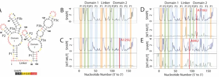
Figure 2.1A illustrates the published secondary structure of the apo Glycine riboswitch based on multiple probing experiments, phylogenetic analysis and partial crystal structures (Butler et al., 2011; Kladwang et al., 2011). The nucleotides are color coded according to
the structure prediction is nearly identical to that of the WT. Not surprisingly, mutating A125 in domain 2 (P3) does not affect structure, as this nucleotide is not paired.
In Figure 2.1D we report the SHAPE-directed prediction for the A116U mutation, which occurs in the P3 helix of domain 2. In this case we see a local difference in the SHAPE trace, and the predicted structure does not contain this region of P3. This mutation has disrupted a single hairpin. It is important to note that the resulting SHAPE differences are readily visualized with the difference of the two traces (green trace, right panel). Figure 2.1E shows the effect of
Figure 2.1 Structure change patterns in SHAPE trace data for glycine riboswitch aptamers
A) Published WT structure for the apo glycine riboswitch aptamers consistent with the crystal structure and multiple independent structure probing experiments (Butler et al., 2011; Kladwang et al., 2011). Red nucleotides indicate high SHAPE reactivity, yellow indicates mid-range reactivity, and black indicates low reactivity. B) The individual WT trace is shown in black; the colored bars indicate the structural regions for each of the aptamers: P1 (orange), P2 (green) and P3 (blue). C) The WT trace (black) is overlaid with the mutant SHAPE trace (dark blue), and the absolute difference between the WT and mutant traces is below (dark green). A red bar on the traces shows the mutation site. The A125U mutation is a mutation that leads to no appreciable differences in structure. 100% of experts that classified this mutant labeled it as a non-changer. D) The A116U mutation leads to a local structure change, where the mutant trace reactivity increases at the mutation site disrupting the P3 region of domain 2. 66% of experts that classified the A116U mutant labeled it as a local changer. E) The A94U mutation leads to a global
2.3.2 Human consensus on local and global structure change
Table 2.1 Expert evaluation summary
Human survey statistics on WT/mutant SHAPE trace pair classification. Survey Statistics
Total Traces 200
Total Experts 14
Total Responses 1427
Mean Trace Coverage 7.24
SD Trace Coverage 2.78
Mean Expert Agreement (%) 79.75
SD Expert Agreement (%) 0.79
Expert Reproducibility (%) 79.70
Total Non-Changers (Majority Consensus) 107
Total Local Changers (Majority Consensus) 40
Figure 2.2 Expert evaluation of RNA structure change in SHAPE data
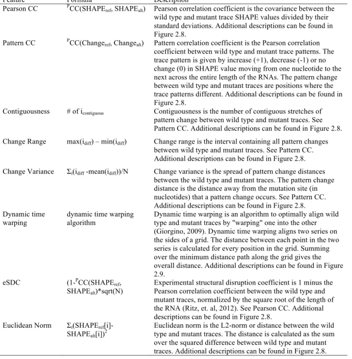
Table 2.2 Features used to quantify differences between WT and mutant traces
Feature formulas and descriptions for the 8 features included in the model. These 8 features were chosen by recursive feature elimination from the total set of 23 features (Methods
Feature Formula Description
Pearson CC PCC(SHAPEref, SHAPEalt) Pearson correlation coefficient is the covariance between the wild type and mutant trace SHAPE values divided by their standard deviations. Additional descriptions can be found in Figure 2.8.
Pattern CC PCC(Changeref, Changealt) Pattern correlation coefficient is the Pearson correlation coefficient between wild type and mutant trace patterns. The trace pattern is given by increase (+1), decrease (-1) or no change (0) in SHAPE value moving from one nucleotide to the next across the entire length of the RNAs. The pattern change between wild type and mutant traces are positions where the trace patterns different. Additional descriptions can be found in Figure 2.8.
Contiguousness # of icontiguous Contiguousness is the number of contiguous stretches of pattern change between wild type and mutant traces. See Pattern CC. Additional descriptions can be found in Figure 2.8. Change Range max(idiff) – min(idiff) Change range is the interval containing all pattern changes
between wild type and mutant traces. See Pattern CC. Additional descriptions can be found in Figure 2.8. Change Variance Σi(idiff -mean(idiff))/N Change variance is the spread of pattern change distances
between the wild type and mutant traces. The pattern change distance is the distance away from the mutation site (in nucleotides) that a pattern change occurs. See Pattern CC. Additional descriptions can be found in Figure 2.8. Dynamic time
warping
dynamic time warping algorithm
Dynamic time warping is an algorithm to optimally align wild type and mutant traces by "warping" one into the other (Giorgino, 2009). Dynamic time warping aligns two series on the sides of a grid. The distance between each point in the two series is calculated for every position in the grid. Summing over the minimum distance path along the grid gives the overall distance. Additional descriptions can be found in Figure 2.9.
eSDC (1-PCC(SHAPEref, SHAPEalt)*sqrt(N)
Experimental structural disruption coefficient is 1 minus the Pearson correlation coefficient between the wild type and mutant traces, normalized by the square root of the length of the RNA (Ritz, et. al, 2012). See Pearson CC. Additional descriptions can be found in Figure 2.8.
Euclidean Norm Σi(SHAPEref [i]-SHAPEalt[i])2
2.3.3 Automated classification of mutation induced structure change
To develop an automated classifier for identifying mutation induced structure changes in RNA we began by establishing a list of 23 features commonly used to evaluate quantitative differences between two linear data sets (Table 2.2 and Table 2.4). Using the human survey classification (Table 2.1) for supervised learning, we trained 38 different algorithms and evaluated their accuracy. The results of this training are provided in Table 2.5 and suggest the Random Forest classifier performs the best on this data using the eight features found in Table 2.2. The trained random forest classifier on these eight features is the algorithm used in the classSNitch R package released with this manuscript.
Interestingly no single feature drives the classification, indicating that the human experts are looking at multiple features of the signal to decide what is or is not a change. Nonetheless we performed random feature elimination and did identify that dynamic time warping alone achieves an accuracy of 65% (Figure 2.10A). Dynamic time warping is less sensitive to distortion caused by local misalignments, a quality that makes the technique useful in speech recognition and likely contributes to the feature’s success in our classifier (Sakoe and Chibe, 1978). We also ranked the eight features by their importance and see that each feature increases accuracy incrementally when added to the model in approximately equal increments. Plotting the WT to mutant Pearson correlation coefficient and contiguousness versus dynamic time warping (Figure 2.10B) reveals how these features correlate but also illustrates subtle differences in how these different features classify change.
data in Figure 2.9B. It identifies the minimum number of insertions and deletions to optimally align the mutant and WT traces. As such, a higher dynamic time warping score indicates greater differences in the traces. It is therefore likely that the expert humans are performing some form of trace alignment combined with pattern matching when evaluating the data. Processing SHAPE data (whether it is obtained by capillary or next generation sequencing) requires an alignment strategy. It is not surprising that humans may choose to ignore small frame shifts in the data (which lead to very high eSDC values) since they know these are most likely errors in trace alignment (Figure 2.11).
Figure 2.3 classSNitch performance
2.3.4 classSNitch analysis of experimental structure change
reaction, it is not surprising that 1M7 can detect more subtle differences in structure that could be occurring on a shorter time scale.
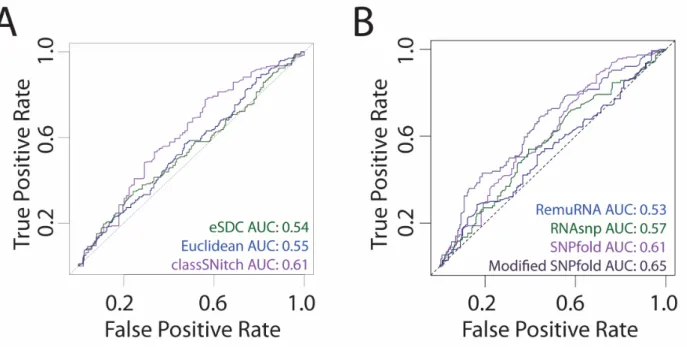
Most structure prediction programs have low accuracy when identifying experimental riboSNitches with AUC values ranging from 0.6-0.7 (Corley et al., 2015; Ritz et al., 2012). In these benchmark studies, validation of the experimental data is analyzed using simple metrics like eSDC or the Euclidean distance (Corley et al., 2015; Ritz et al., 2012). One possible
explanation for the poor predictive performance of the prediction algorithms in these benchmark studies is misclassification of the experimental data with these simple metrics. Indeed, when we observe the performance of SNPfold on data classified with either eSDC or Euclidean difference, the AUC values indicate the algorithm is barely predictive (Figure 2.5A). We observe a subtle improvement in performance when we use the classSNitch classification of the experimental data. A similar performance increase is observed for the other published algorithms designed for riboSNitch prediction (Figure 2.5B) (Halvorsen et al., 2010; Sabarinathan et al., 2013; Salari et al., 2013). Thus, misclassification of experimental data is likely a confounding factor for the poor performance of riboSNitch prediction algorithms, and the use of classSNitch in future benchmarking studies may improve prediction accuracy. Details on algorithm parameters can be found in Methods Supplementary, section 2.5.3.4.
2.3.5 WT SHAPE informed riboSNitch detection
It is well established that incorporating SHAPE into RNA structure folding algorithms improves secondary prediction performance (Diegan et al., 2009). Since we use SHAPE data to detect riboSNitches, it does not make sense to include experimental data for the WT and mutant in structure predictions. Nonetheless our analysis of sequence composition and WT SHAPE data for local and global changers does suggest an alternative. Can the WT SHAPE trace alone inform riboSNitch predictions? This is an attractive strategy since ultra high-throughput techniques exist to collect WT data on a genome-wide scale (Siegfried et al., 2014).
The major bottleneck in collecting systematic mutational information is the molecular biology required to synthesize and validate each mutant. When we modify the SNPfold
Figure 2.4 Fraction of disruption for individual RNAs
A) The fraction of mutations that cause no change (red), local change (blue) or global change (green) for each RNA as classified by classSNitch. The RNAs are grouped by biological
2.4 Discussion
Identifying mutations that are likely to lead to changes in RNA structure remains a significant computational and experimental challenge (Chauhan and Woodson, 2008; Cheng et al., 2005; Churkin et al., 2011; Russell et al., 2002). Such predictions are important in the context of personalized medicine since many riboSNitches are now known to be causative of human disease (Solem et al., 2015). Despite the advent of experimental technology enabling us to probe structure on a genome-wide scale, we still rely on structure change prediction
algorithms or visual interpretations of the data to detect riboSNitches as there is no ultra-high throughput approach for rapidly mutating an RNA (Ritz et al., 2012; Rocca-Serra et al., 2011; Sansone et al., 2012; Siegfried et al., 2014).
We hypothesized that one reason for the poor performance of RNA structure prediction algorithms (Corley et al., 2015; Ritz et al., 2012) on riboSNitches is the misclassification of the experimental data. We therefore set out to develop novel metrics to evaluate structure change from SHAPE data. This approach did lead to modest improvements in performance suggesting that careful analysis of SHAPE data is essential when using these data as a benchmark. In this age of whole transcriptomic structure probing, manual validation and curation of these data sets is impractical. The classSNitch classifier simulates human consensus on what is and is not a structure change and therefore offers an alternative to simple metrics like eSDC in
Figure 2.5 Improving the performance of structure change prediction algorithms
A) We performed ROC curve analysis for SNPfold, a structure change prediction algorithm, using classSNitch (purple), eSDC (green) and the Euclidean norm (blue) to classify the experimental data using the 10% tails strategy (Corley et al., 2015). B) We compare the performance of structure change prediction algorithms on the classSNitch classification for SNPfold (purple), RNAsnp (green) and RemuRNA (blue). Each of these algorithms predicts structure change in RNA using only sequence information. SNPfold, remuRNA, and RNAsnp all make ab initio predictions on whether a mutation alters the RNA structure; none of the
The features that classSNitch uses to classify change reveals some of the subtleties involved in interpreting SHAPE data. Beyond evaluating the magnitude difference between traces, human experts also utilize information on pattern matching and the distribution of change along the length of the RNA (Figures 2.8 and 2.9). We used those features to develop a classifier that successfully mimics expert classification of structure change (Figure 2.3). SHAPE reactivity is correlated with secondary structure, more reactive nucleotides are generally single stranded (Eddy, 2014); however the experiment probes the overall structure of the RNA. The classSNitch classifier does not attempt to model structure, but instead establishes a standard for quantifying change. This is biologically relevant, allowing us to compare different RNAs using a standard vocabulary (Figure 2.4). Although only two synthetic RNAs are included in our data set, there is a striking difference in their sensitivity to mutation (Figure 2.4A). Indeed a much larger fraction of the mutations in these RNAs result in conformational rearrangement. Although with only two RNAs it is impossible to draw statistical conclusions, this observation remains biologically interesting and warrants further investigation as more experimental data is obtained on a wide variety of RNAs (both synthetic and naturally occurring). The idea that RNA sequences under natural evolutionary pressure may evolve a general robustness to mutation warrants further investigation.
The data used for training classSNitch was exclusively collected using traditional
capillary methods of electrophoresis. The quantification of this type of data from a capillary trace
is a challenge, as it requires alignment to a reference ladder (Das et al., 2005; Karabiber et al.,
2013; Mitra et al., 2008). Recent algorithmic developments have further automated this process
and increased reliability (Yoon et al., 2011). It is interesting that dynamic time warping is the
errors were to persist in the data, one might expect that experts could be correcting these when
gazing at the data. As technology has evolved, in particular with the use of next generation
sequencing to collect chemical and enzymatic probing data (Kertesz et al., 2010; Mortimer et al.,
2012; Rouskin et al., 2014; Siegfried et al., 2014) alignment artifacts may disappear in the data.
As such it may become necessary to retrain classSNitch on these newer types of data. In our lab’s limited experience with these types of data (currently unpublished), classSNitch
Although classSNitch was trained on riboSNitches and is primarily intended as a tool to evaluate the effect of mutation induced structure change, it is in fact a more general metric for comparing SHAPE data. RNAs will adopt alternative conformations depending on their
environment. For example riboswitches adopt different conformations depending on the presence of the ligand. When applied to the WT traces of apo and bound riboswitch data, the algorithm does identify local and global change for a majority of riboswitches, as expected. Protein binding, changes in cellular environment and even counter-ions are known to affect RNA structure (Bai et al., 2005; Frederiksen et al., 2012). The classSNitch classifier provides a common language to describe these differences. For example, it could be used when comparing in vivo and in vitro probing of the RNA to identify regions where the presence of proteins alters structure locally and globally. It also offers an attractive way to quantify these changes in agreement with expert consensus.
The agreement between human experts “gazing” at this data is reassuring. Prior to quantitative methods being widely available to life scientists, significant progress was achieved by carefully looking at the data; the structure of group I introns, tRNA, and the ribosome were correctly predicted manually years before the were crystallized (Michel and Westhof, 1990). The value of automated systems that reproduce human appreciation of data is underutilized in RNA structural research despite the rich history of success in the field. Developing the classSNitch classifier minimally captures dying expert knowledge, while also making this expertise accessible to the community in an automated package.
2.5 Methods Supplementary
2.5.2 Methods
2.5.2.2 Data normalization and noise reduction
Variables:
n = nucleotide position
N = trace length in nucleotides WT = wild type reactivities MT = mutant reactivities
WTnorm = normalized wild-type trace MTnorm = normalized mutant trace WTreduc = noise reduced
MTreduc = noise reduced
Normalization: We normalized the mean of every WT trace to a mean of 1.5. This step increases the mean of the WT traces so that differences in magnitude are more pronounced.
𝑊𝑇𝑛𝑜𝑟𝑚 = 1.5𝑁 Σ𝑊𝑇 ∗𝑊𝑇 (9)
We normalized each MT by the multiplier that minimizes the absolute difference between the WT and MT. This step minimizes small differences in magnitude between the WT and MT traces that may be attributable to noise.
𝑀𝑇𝑛𝑜𝑟𝑚= 𝑎𝑟𝑔𝑚𝑖𝑛! Σ( 𝑊𝑇−𝑥∗𝑀𝑇 ) ∗𝑀𝑇 (10)
Noise Reduction: For every nucleotide [n], if the value in both WT and MT are higher than the normalized “high reactivity” value determined by QuSHAPE, we set MT[n] equal to WT[n]. This step minimizes differences in magnitude when both WT and MT have high reactivity.
if (WTnorm[n] > HIGH & MTnorm[n] > HIGH){MTreduc = WTreduc} (11)
For every nucleotide [n], if the value is less than -0.5, set them equal to 0. This step minimizes differences in magnitude when both WT and MT have small reactivity.
2.5.2.3 Human expert evaluations
Non-changer: A mutation that leads to no difference between the wild type and mutant SHAPE traces. Small differences at the mutation site or the two nucleotides immediately adjacent to the mutation site may be caused by a difference in reactivity between the modifier and specific nucleotide types. Due to this difference, changes in this region are ignored.
Local changer: A mutation that leads to a difference between the wild type and mutant SHAPE traces in the 20-nucleotide region surrounding the mutation site (10 nucleotides on either side). This is the average region of change around the mutation site for mutants labeled as local changers by the experts.
Global changer: A mutation that leads to differences between the wild type and mutant SHAPE traces beyond the 20-nucleotide region surround the mutation site. The change may be contiguous or separated by some distance and may also include change around the mutation site. 2.5.2.4 Feature and algorithm selection
k-fold cross-validation (CV): CV is a method used for model validation. In CV the data is divided into k subsamples. k-1
same 5 subsets were used for validation of every algorithm. The traces used in the validation folds are further described in Table 2.8. Random forest performed the best across validation for local, global and non-changers. Since the available number of manually classified samples was limited, we decided to average the performance over the 5 cross-validation sets (Brun et al., 2008; Molinaro et al., 2005).
Recursive Feature Elimination (RFE): RFE is a method for choosing a subset of appropriate features for use in a predictive model (Kuhn, 2008; Saeys et al., 2007; Zhou et al., 2014). We initially built a random forest model using all 23 features. To rank the features, we used
permutation importance, which measures the mean decrease in accuracy when a feature’s values are shuffled (Kuhn, 2008; Saeys et al., 2007; Zhou et al., 2014). We systematically remove one feature and retrain the models. This recursive process effectively ranks the feature’s importance when repeated, in our case, 10 times. Each time the order of the features remained the same, but the cumulative accuracy varied. Averaging the cumulative accuracy over 10 runs, we selected the number of features beyond which
the cumulative accuracy stabilized (the accuracy no longer increased). Thus this procedure allows us to identify the seven features we ultimately
implemented in the classSNitch
classifier. To perform recursive feature analysis, we used the rfeControl and
Random Forest (RF): Random Forest is a supervised learning technique using decision trees that can be used for classification or regression (Breiman, 2001; Liaw and Wiener, 2002). A decision tree groups the samples into different nodes according to the feature being measured. The root node includes all of the samples. In the first step a feature is selected at random and used to split the tree. The tree grows by choosing the best split based on the selected feature and breaking the samples into two new nodes. A node that can no longer be split is called a leaf node, because all samples are identical or the node only contains a single sample. Leaf nodes may contain samples with a mixture of expert class labels. For each sample, the tree “votes” on a class based on the majority of class labels in the leaf node where it is found. This is a supervised learning algorithm where the expert classifications determine the best tree from which to build the classifier. Random forest uses a set or forest of these decision trees (Breiman, 2001; Liaw and Wiener, 2002). Each individual tree samples with replacement from the full set of data, such that each tree is built on a different subset. Due to this sampling, trees may disagree on class votes for individual samples. The class for each sample is determined by the majority vote among all of the trees. Sampling with replacement results in some data being left out of the tree, referred to as “out-of-bag”. Each tree can predict the class for its “out-of-bag” samples. The classification error for the out of bag samples gives the generalization error. The classification for new samples can be determined from an existing forest of trees (Breiman, 2001; Liaw and Wiener, 2002). We chose a number of random forest trees greater than the number beyond which the error rate (averaged over 10 runs) stabilized.
optimization are those reported in Table 2.5. The optimization for random forest is described above. KStar is an instance-based learner that assigns classes for new instances according to its k-nearest data points (Cleary and Trigg, 1995). Similarity between samples in KStar is
determined by entropy. By gradually increasing the global blending parameter, we found the value that resulted in the maximum number correctly classified for non-changers, 22%.
Multilayer perceptron is an artificial neural network (Silva et al., 2008). The algorithm consists of layers of nodes in a directed graph, where each node is a nonlinear activation function. In multilayer perceptron the network is trained through backpropagation using gradient descent. We determined the optimal learning rate, momentum number of hidden layers and number of nodes in a given layer by gradually increasing each parameter individually and leaving the others at their default setting. The optimal learning rate was 0.1, the momentum was 0.65, the number of hidden layers was 1, and the single hidden layer had 5 nodes.
2.5.2.6 WT SHAPE improved SNPfold
SNPfold.py -A <seq file> <mutation> (14)
2.5.2.7 Figures and Diagrams
The minimum free energy structures were predicted using the RNAstructure package suite with SHAPE data to constrain the prediction (Diegan et al., 2009; Matthews, 2004; Matthews et al., 2004). Structure diagrams were created using VARNA (Darty et al., 2009). Cobweb diagrams were used for multi-class performance analysis (Diri and Albayrak, 2008).
2.5.3 Results
2.5.3.4 classSNitch analysis of experimental structure change
RNAsnp: We used default parameter settings for mode 1 (global folding) with RNAsnp (Sabarinathan et al., 2013). The window size for including base pairing probabilities is 200 nucleotides on either side of the mutation. We used the p-value for the correlation coefficient as the measure.