Vol. 11 (2017) 4179–4219 ISSN: 1935-7524
DOI:10.1214/17-EJS1355
Multiscale inference for multivariate
deconvolution
Konstantin Eckle
University of Leiden Mathematical Institute 2333 CA Leiden, The Netherlands e-mail:[email protected]
Nicolai Bissantz and Holger Dette
Ruhr-Universit¨at Bochum Fakult¨at f¨ur Mathematik 44780 Bochum, Germany
e-mail:[email protected];[email protected]
Abstract: In this paper we provide new methodology for inference of the geometric features of a multivariate density in deconvolution. Our approach is based on multiscale tests to detect significant directional derivatives of the unknown density at arbitrary points in arbitrary directions. The mul-tiscale method is used to identify regions of monotonicity and to construct a general procedure for the detection of modes of the multivariate density. Moreover, as an important application a significance test for the presence of a local maximum at a pre-specified point is proposed. The performance of the new methods is investigated from a theoretical point of view and the finite sample properties are illustrated by means of a small simulation study.
MSC 2010 subject classifications:Primary 62G07, 62G10; secondary 62G20.
Keywords and phrases:Deconvolution, modes, multivariate density, mul-tiple tests, Gaussian approximation.
Received November 2016.
Contents
1 Introduction . . . 4180
2 Multiscale inference in multivariate deconvolution . . . 4182
3 Asymptotic properties . . . 4185
4 Finite sample properties . . . 4190
4.1 A local test for modality – testing for a single mode . . . 4191
4.2 A local test for modality – testing for two modes simultaneously 4194 4.3 Inference about local monotonicity of a multivariate density . . 4196
5 Proof of Theorem3.1. . . 4196
5.1 Auxiliary results . . . 4197
5.2 Proof of the approximation (3.8) . . . 4203
5.2.2 Proof of (5.9) . . . 4208
5.3 Boundedness of the approximating statistic . . . 4209
6 Proofs of Theorems3.2and3.3 . . . 4215
7 Two technical results . . . 4217
Acknowledgements . . . 4217
References . . . 4218
1. Introduction
In many applications such as in biological, medical imaging or signal detec-tion only indirect observadetec-tions are available for statistical inference, and these problems are called inverse problems in the (statistical) literature. In the case of medical imaging, a well-known example is Positron Emission Tomography. Here, the connection between the ‘true’ image and the observations involves the Radon transform [see, for example, [10]]. Other typical examples are the reconstruction of biological or astronomical images, where the connection between the true image and the observable image is - at least in a first approximation - given by convolution-type operators [see, for example, [2] or [5]]. Whereas in these models the data is in general described in a regression framework, similar (de-) convolution problems arise in density estimation from indirect observations [see [13] for an early reference]. The corresponding (multivariate) statistical model for density deconvolution is defined by
Yi=Zi+εi, i= 1, . . . , n, (1.1)
where (Z1, ε1), . . . ,(Zn, εn)∈ Rd×Rd are independent identically distributed
random variables and the noise terms ε1, . . . , εn are also independent of the
random variablesZ1, . . . , Zn. We assume that the densityfεof the errorsεi is
known and are interested in properties of the densityf of the random variables Zi based on the sample{Y1, . . . , Yn}. In terms of densities, model (1.1) can be
rewritten as
g=f∗fε,
where g denotes the density of Y1. Density estimators can be constructed and
investigated similarly to the regression case (see the references in the next para-graph), and in this paper we are interested in describing qualitative features of the densityf using the sample {Y1, . . . , Yn}. In particular we will develop a
method for simultaneous detection of regions of monotonicity of the density f at a controlled level and construct a procedure for the detection of the modes of f. To our best knowledge multivariate problems of this type have not been investigated so far in the literature.
parameter for the noise level]. [6] develop confidence bands for deconvolution kernel density estimators, while minimax rates for this estimation problem can be found in [9] and [16]. [28] and [18] point out that the detection of regions of monotonicity and of the modes of a density is a more complex problem and [16] shows that the minimax rate for estimating the derivative over a H¨ older-β-class (β ≥ 2) in the univariate setting d= 1 is given by n−(β−1)/(2β+2r+1),
where r >0 denotes the order of polynomial decay of the Fourier transform of the error density fε. [3] develop a test for the number of modes of a univariate
density and [25] proposes a local test for monotonicity for a fixed interval. More recently [30] discuss multiscale tests for qualitative features of a univariate den-sity which provide uniform confidence statements about shape constraints such as local monotonicity properties. These authors use a Koml´os-Major-Tusn´ady (KMT) estimate for the empirical process (cf. [22]). As the classical KMT con-struction is not suitable for multivariate multiscale problems because it imposes rather strong conditions, it is not obvious how to analyze multiscale inference in a multivariate context. In the present paper we present a solution of this problem. In particular, we use recent results on Gaussian approximations of multivariate empirical processes [[11]] to address this problem. Multiscale test-ing is also widely used in spatial testtest-ing, see [24] and [31], among others. Here, one aims at the detection of geometric objects of activation in a grid of sensors with noisy measurements and makes use of limit distributions of suprema of sums of i.i.d. Gaussian random variables [cf. e.g. [20]].
Little research has been done regarding multivariate deconvolution problems. Recent references for density estimation are e.g. [12] using kernel density esti-mators and [29] for a Bayesian approach in the case of an unknown error distri-bution with replicated proxies available. Hypothesis testing in deconvolution is investigated in [19] and [7].
In the present paper we will develop a multiscale method for simultaneous identification of regions of monotonicity of the multivariate density f in the deconvolution model (1.1). As we do not impose any conditions or even assume prior knowledge about the shape of the density, our problem and approach differ substantially from the methods used in shape-constrained density estima-tion [see for example [27] and [4], among others, for some references on shape-constrained density estimation]. In contrast to shape-shape-constrained inference, our approach is based on simultaneous local tests of the directional derivatives of the densityf for a significant deviation from zero for “various” directions and locations.
and all proofs are deferred to Sections 5 and 6, while Section 7 contains two technical results.
2. Multiscale inference in multivariate deconvolution
Let ∂s denote the directional derivative in the direction of s ∈ Sd−1 = {s ∈
Rd| s= 1}andφ:Rd→R
≥0be a sufficiently smooth kernel (i.e.φL1(Rd)= 1) with compact support in [−1,1]d. From a theoretical point of view, only assumptions on the smoothness of φ have to be imposed and therefore, the theoretical part of this paper investigates arbitraryφ. For practical applications, the functionφcan be chosen e.g. as a radially symmetric kernel which does not favor any directions, or as a polynomial kernel such as used in the simulations in Section4. However, this choice has to be made in advance, and φmust be fixed throughout the data analysis. Define
φt,h(.) =h−dφ
.−t
h
fort∈[0,1]d, h >0.
For the description of the local monotonicity properties of the function f we introduce the integral
−
Rd
∂sf(x)φt,h(x) dx. (2.1)
If this expression is, say, negative, we can conclude that the derivative of f in direction shas to be strictly larger than zero on a subset of positive Lebesgue measure of the cube [t1−h, t1+h]×. . .×[td−h, td+h]. Ideally, one would
inves-tigate directly the directional derivatives off for statistical inference regarding its monotonicity properties. However, the estimation of derivatives is difficult, especially in the deconvolution framework of this paper, such that we consider instead the integral (2.1). Note that for h approaching zero the integral (2.1) approximates the directional derivative−∂sf(t).
In most applications no prior knowledge about the densityf is available and therefore, one would like to test for all triples (s, t, h) consisting of all directions s, locationstand scaling factorsh. As this is impossible, we choose a finite set of triplesTn :={(sj, tj, hj)| j = 1, . . . , p} and estimate the integral (2.1) for
every (sj, tj, hj)∈Tn simultaneously. For statistical inference we then propose
a multiscale testing procedure. The practical choice ofTn depends on the task
considered by the experimenter, but typically the choice of an equidistant grid is reasonable. We present below two examples to chooseTn to obtain a graphical
representation of the density and to obtain a local mode test, respectively. Statistical inference regarding the monotonicity properties off is performed by testing simultaneously several hypotheses of the form
Hsj,tj,hj
0,incr :−
Rd
∂sjf(x)φtj,h
j(x) dx≥0
versus
Hsj,tj,hj
1,incr :−
Rd
∂sjf(x)φtj,h
j(x) dx <0
and
Hsj,tj,hj
0,decr :−
Rd
∂sjf(x)φtj,hj(x) dx≤0 versus
Hs j
,tj,hj
1,decr :−
Rd
∂sjf(x)φtj,hj(x) dx >0
(2.3)
for (sj, tj, h
j)∈Tn, where the inference is based on estimates of allpintegrals
Rd
∂sjf(x)φtj,hj(x) dx, j= 1, . . . , p,
see (2.6) below for the estimators. Testing simultaneously means that the same dataset Yi, i = 1, . . . , n, is used for inference about all 2p hypotheses in (2.2)
and (2.3), and that we consider the overall error level for at least one false rejection over all tests. To take the multiple testing problem into account, we propose below an investigation of the joint distribution of thepestimates. This approach allows us to control the family wise error rate of the 2ptests for the hypotheses (2.2) and (2.3). Moreover, we can choosepmuch larger thann, such that standard correction procedures of thep-value in multiple testing problems such as Holm-Bonferroni or False Discovery Rate do not apply.
The method allows for a global understanding of the shape of the densityf. A particular feature of the proposed method consists in the fact that by conducting formal statistical tests the multiple level can be controlled (see Theorem3.2). To be precise, define by Tincr
n the set of all triples inTn for which the hypothesis
(2.2) is rejected, and byTdecr
n the set of all triples inTnfor which the hypothesis
(2.3) is rejected. Then the probability of at least one false rejection within the setsTincr
n andTndecrcan be bounded by a pre-determined error rateα∈(0,1),
that is, the method allows to conclude that with probability≥1−αit holds
−
Rd
∂sjf(x)φtj,h
j(x) dx <0 for all (s
j, tj, h
j)∈Tnincr
and
−
Rd
∂sjf(x)φtj,h
j(x) dx >0 for all (s
j, tj, h
j)∈Tndecr.
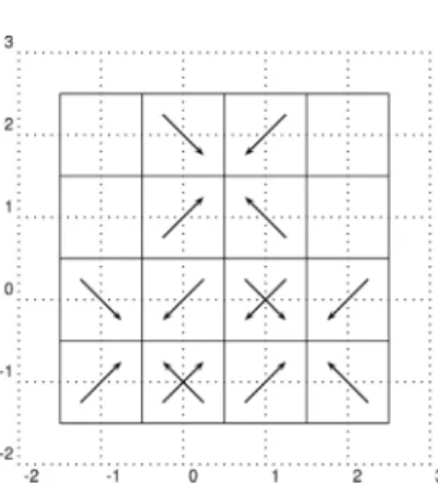
For example, simultaneous tests for hypotheses of the form (2.2) and (2.3) can be used to obtain a graphical representation of the local monotonicity behavior of the density as displayed in Figure1for a bivariate density. The displayed map is based on tests for the hypotheses (2.2) for a fixed scaleh0and different locations
and directions (s1, t1), . . . ,(sp, tp) (here taken as the vertices of an equidistant grid and four equidistant directions onS1). Note that we are investigating here a symmetric set of triples, that is, for every locationtj both the triple (sj, tj, h
0)
and (−sj, tj, h
0) are considered. Thus, asHs
j,tj,h
0
0,incr =H− sj,tj,h
0
0,decr , it is sufficient to
Fig 1. Example of a global map for monotonicity of a bivariate density.
at a locationtj represents a rejection of the corresponding hypothesisHsj,tj,h
0
0,incr
and provides therefore an indication of a positive directional derivative off in directionsj at the locationtj. For a detailed description of the settings used to
provide Figure1 and an analysis of the results we refer to Section4.3.
If one is interested in specific shape constraints of the density, say in a test for a mode (local maximum) at a given point x0, inference can be conducted investigating the hypotheses
Hsj,tj,h0
0,decr versus H
sj,tj,h
0
1,decr (2.4)
for different pairs (t1, s1), . . . ,(tp, sp), wheret1, . . . , tp are points in a neighbor-hood ofx0on the lines{x0+λsj|λ >0} (j= 1, . . . , p), respectively (of course,
on could additionally use different scales here).
Throughout this paper we will assume that all partial derivatives ∂sf of
the density f are uniformly bounded, such that the estimated quantity (2.1) is bounded by a constant which does not depend on the triple (s, t, h). Using integration by parts, Plancherel’s identity and the convolution theorem, we get
−
Rd
∂sf(x)φt,h(x) dx=
Rd
f(x)∂sφt,h(x) dx (2.5)
= 1
(2π)d
Rd
F(f)(y)F(∂sφt,h)(y) dy
= 1
(2π)d
Rd
F(g)(y)
F(∂sφt,h)
F(fε)
(y) dy
=
Rd
g(x)F−1
F(∂sφt,h)
F(fε)
(x) dx.
Here,
F(f)(y) =
Rd
F−1(f)(x) = 1
(2π)d
Rd
eix.yf(y) dy x, y∈Rd
denote the Fourier transform and its inverse, respectively, z is the complex conjugate ofz∈Candx.ystands for the standard inner product ofx, y∈Rd.
For the construction of tests for the hypotheses in (2.2) and (2.3) we define the statistic
Ts,t,hn = 1 n
n
i=1
Fs,t,h(Yi), (2.6)
where
Fs,t,h(Yi) =F−1
F(∂
sφt,h)
F(fε)
(Yi). (2.7)
Because (by (2.5))
E(Tn
s,t,h) =−
Rd
∂sf(x)φt,h(x) dx,
it follows thatTn
s,t,his a reasonable estimate of the quantity defined in (2.1), and
hence the statistics Ts,t,hn define the main tool to study qualitative features of the densityf. Inference on local monotonicity of the densityfwill then be based on tests rejecting the hypotheses H0,incrs,t,h for small values of the corresponding statisticTs,t,hn and rejectingH0,decrs,t,h for large values ofTs,t,hn for several directions s∈Sd−1, locationst∈[0,1]dand scalesh >0. The multiple level of these tests
can be controlled by investigating the (asymptotic) maximum of appropriately normalized statistics Tn
s,t,h calculated over a certain set of locations, directions
and scales.
3. Asymptotic properties
In this section we investigate the asymptotic properties of a statistic which can be used to control the multiple level of the tests introduced in Section2. To be precise, we consider the finite subset
Tn:=
(sj, tj, hj)|j= 1, . . . , p
⊆Sd−1×[0,1]d×[hmin, hmax]
of cardinality p ≤ nK for the calculation of the maximum of appropriately standardized statisticsTs,t,hn , whereK >1 and for someε >0
hminn−1/d+ε and hmax=o((log(n) log log(n))−1). (3.1)
Throughout this paper we will make frequent use of multi-index notation, where
α= (α1, . . . , αd)∈Nd0 denotes a multi-index (written in bold),|α|=α1+. . .+
αd its “length”, and for a sufficiently smooth functionf :Rd→Rand a
multi-index αwe denote by
∂αf(x) = ∂ |α|
∂xα1
1 ·. . .·∂xαdd
f(x)
Recall the definition ofFs,t,h in (2.7) and to simplify the notation define for
a point (sj, tj, h j)∈Tn
Fj=Fsj,tj,h
j. (3.2)
The testing procedure for the hypotheses (2.2) and (2.3) is based on the p estimatesTn
sj,tj,h j =
1 n
n
i=1Fj(Yi) in 2.6for the integrals
E(Tn
sj,tj,hj) =E(Fj(Y1)) =−
Rd
∂sjf(x)φtj,h
j(x) dx, j= 1, . . . , p. For a rigorous statistical test which controls the multiple level we therefore need to investigate the asymptotic joint distribution of
√
nTsnj,tj,hj−E(Tsnj,tj,hj)= 1
√
n
n
i=1
Fj(Yi)−nE(Fj(Y1)), j= 1, . . . , p.
(3.3)
Recall thatpis growing withn. Thus, the maximum over allprandom variables in (3.3) is in general not bounded. As a consequence, the random variables de-fined in (3.3) have to be properly standardized. It turns out that the approriate standardization is given by
˜ Xj(1)=
log(eh−jd)
log log(eeh−d j )
hd/2+r+1
j
√
nˆgn(tj)Vj
n
i=1
Fj(Yi)−nE(Fj(Y1))−
(3d−1) log(h−jd) , (3.4) where ˆgn is a density estimator ofg satisfying
g−gˆn∞=o(log(n)−1) almost surely (3.5)
(for example a kernel density estimator as considered in [17]) and
Vj=hd/2+r+1j Fsj,tj,hjL2(Rd). (3.6) The quantity Vj is well-defined under the assumptions presented below (see
Lemma5.2for details).
Note that the boundary of the hypothesesHs j
,tj,hj
0,incr andH sj,tj,hj
0,decr in (2.2) and
(2.3) is defined byRd∂sjf(x)φtj,hj(x) dx= 0 and in this case we have 1
√
nX˜
(1)
j =
log(eh−jd)
log log(eeh−d j )
hd/2+r+1
j
√
ˆ gn(tj)Vj
Tsnj,tj,hj−
(3d−1) log(h−jd) √
n .
Consequently, we will investigate the asymptotic properties of max1≤j≤pX˜j(1)in
the following discussion. For this purpose we make the following assumptions.
Assumption 1. Assume that the densityg is Lipschitz continuous and locally bounded from below, i.e.
Assumption 2. We assume a polynomial decay of the Fourier transform of the error densityfε, i.e. that there exist constantsr >0 ford≥2 resp.r > 12 for
d= 1 and 0< Cu< Co such that
Cu
1 +y2−r/2≤ |F(fε)(y)| ≤Co
1 +y2−r/2. Furthermore, let
(d+1)/2
j=1
(1 +y2)j/2 ∂j
∂yljF(fε)(y)
≤Co(1 +y2)−r/2
for alll= 1, . . . , d.
Note that as a direct consequence of Assumption1g is bounded from above and that there exists a constant δ > 0 such that g(x) ≥ c
2 > 0 for allx ∈
[−δ,1 +δ]d. Assumption 2 can be seen as a multivariate generalization of the
classical assumptions on the decay of the Fourier transform of the error density in the ordinary smooth case (see e.g. [30], Assumption 2). We also note that this assumption defines a mildly ill-posed situation (see [7]). The next assumptions refer to the kernelφand are required for some technical arguments.
Assumption 3. Let ∂sφL2(Rd) = 0 for all s ∈ Sd−1 and assume that ∂βφ exists in [−1,1]d and is continuous for all|β| ≤ r+ 2, whereris the constant
from Assumption2. We assume further that for someδ >0 the inequality
Rd
1 +y2r+(d+δ)/2 ∂
m
∂ym l
F(∂ekφ)(y)
2
dy <∞
holds for all k, l= 1, . . . , dandm= 0, . . . ,(d+ 1)/2, whereek, k= 1, . . . , d,
denotes thekth unit vector ofRd.
As
∂m
∂ym l
F(∂sφ)(y) 2
=
d
k=1
sk
∂m
∂ym l
F(∂ekφ)(y) 2
≤C
d
k=1
∂m
∂ym l
F(∂ekφ)(y) 2
for alls∈Sd−1and some constantC >0 that only depends ond, Assumption 3 yields a uniform upper bound for the integral
Rd
1 +y2r+(d+δ)/2 ∂
m
∂ym l
F(∂sφ)(y) 2
dy
for alls∈Sd−1.
Recall the definition of ˜Xj(1) in (3.4) and define the vector ˜
X(1)= ( ˜X1(1), . . . ,X˜p(1)).
Our first main result provides a uniform approximation of the probabilities P( ˜X(1) ∈A) by the probabilitiesP( ˜X ∈A) for every half-open hyperrectangle
˜ Xj =
log(eh−jd)
log log(eeh−d j )
hd/2+r+1j |
RdFj(x) dBx|
Vj −
(3d−1) log(h−jd) (3.7)
(j = 1, . . . , p), and (Bx)x∈Rd is a standard d-variate Brownian motion. The limit process ˜X is constructed in such a way that it has (asymptotically) the same covariance structure as the vector ˜X(1) consisting of all test statistics.
Moreover, the process ˜Xj does not depend on unknown quantities. In order
to construct quantiles for the testing procedure for the hypotheses (2.2) and (2.3), we consider the quantity max1≤j≤pX˜j and use Theorem (3.1) below to
show that the quantiles of max1≤j≤pX˜j(1) can be approximated by those of
max1≤j≤pX˜j (note that this is a simple consequence of Theorem3.1, using the
the setA = (−∞, a]×(−∞, a]× ×. . .(−∞, a]). Theorem 3.1. Let A denote the set
A :={(−∞, a1]×. . .×(−∞, ap]|a1, . . . , ap∈R}. Then,
sup
A∈A
P˜
X(1)∈A−PX˜ ∈A=o(1) forn→ ∞. (3.8)
Furthermore, the random variable max1≤j≤pX˜j is almost surely bounded uni-formly with respect ton.
Theorem3.1 will be used to control the multiple level of statistical tests for the hypotheses of the form (2.2) and (2.3). To this end, letα∈(0,1) and denote byκn(α) the smallest number such that
P max
1≤j≤p
˜
Xj ≤κn(α) ≥1−α. (3.9)
By Theorem 3.1, κn(α) is bounded uniformly with respect to n. The jth
hy-pothesis in (2.2) is rejected, whenever
n−1
n
i=1
Fj(Yi)<−κjn(α), (3.10)
where
κjn(α) =
√
ˆ gn(tj)Vj
√
n h
−d/2−r−1 j
log log(eeh−d j )
log(eh−jd) κn(α) +
(3d−1) log(h−jd) . (3.11) Similarly, thejth hypothesis in (2.3) is rejected, whenever
n−1
n
i=1
Fj(Yi)> κjn(α). (3.12)
Note that the ill-posedness of the deconvolution problem is reflected in the value of the quantile κj
n(α) through the multiplication with h−jr and by the
Theorem 3.2. Assume that the tests(3.10)and (3.12)for the hypotheses (2.2)
and (2.3) are performed simultaneously for j = 1, . . . , p. The probability of at least one false rejection of any of the tests is asymptotically at most α, that is
P∃j∈ {1, . . . , p}: n−1|
n
i=1
Fj(Yi)|> κjn(α) ≤α+o(1)
forn→ ∞.
Remark 3.1. It is a well-known fact that statistical inference regarding the qualitative features of a multivariate density is a challenging problem from a computational point of view. In the present context conducting all tests (3.10) and (3.12) for the hypotheses (2.2) and (2.3) is computationally demanding. In general, the support of the deconvolution kernel Fj is not compact and
there-fore, the computation of allptest statistics consists ofp·nkernel evaluations. The computation of the covariance matrix RdFj(x)Fk(x) dx
j,k=1,...,p of the
Gaussian limit process depends on p·(p+ 1)/2 numerical integrations and for the determination of the quantiles of the limit process p-dimensional normal distributed random vectors have to be simulated.
Next we introduce a method for the detection and localization of the modes of the density. The main idea is to conduct the local tests for modality proposed in (2.4) for a set of candidate modes which does not assume any prior knowledge about the density. To be precise, we assume the following condition on the set Tn: for any fixedhandsthe set{t: (s, t, h)∈Tn}is an equidistant grid in [0,1]d
with grid widthh. Furthermore, for any fixedtandhthe set{s: (s, t, h)∈Tn}
is a grid inSd−1with grid width converging to zero with increasing sample size.
This grid is now used as follows to check if a pointx0∈(0,1)dis a mode off.
LetTx0
n ⊂Tn be the set of all triples (s, t, h)∈Tn such thatch≥ x0−t ≥
2√dh for somec >2√dsufficiently large and angle(t−x0, s)→0 forn→ ∞.
By the condition onTn defined above, the setTx
0
n is nonempty for sufficiently
large n. We now use the local tests (3.12) for the hypotheses (2.4) and decide for a mode at the point x0 if the null hypotheses in (2.4) are rejected for all
triples in Tx0
n simultaneously. Note that by choosing the test locations as the
vertices of an equidistant grid no prior knowledge about the location of x0 has
to be assumed. Theorem3.3below states that the procedure detects all modes of the density with asymptotic probability one as n→ ∞.
Theorem 3.3. Let x0∈(0,1)d denote an arbitrary mode of the density f and assume that there exist functions gx0 : Rd → R, f˜x0 : R → R such that the densityf has a representation of the form
f(x)≡(1 +gx0(x)) ˜fx0(x−x0) (3.13) (in a neighborhood ofx0),g
x0 is differentiable in a neighborhood of the pointx0 such that both gx0(x) =o(1) and ∇gx0(x), e=o(x−x0)if x→x0 for all
e∈Rd with e = 1. In addition, let f˜
If the set
(s, t, h)∈Tn:h≥Clog(n)1/(d+2r+4)n−1/(d+2r+4)
for some C > 0 sufficiently large is nonempty, then the procedure described in the previous paragraph detects the mode x0 with asymptotic probability one as
n→ ∞.
The method to detect the modes of the density proposed in Theorem 3.3 proceeds in two steps: the verification of the presence of a mode with asymptotic probability one in the asymptotic regime presented above and its localization at the raten−1/(d+2r+4) (up to some logarithmic factor) given by the grid width.
[16] showed that in the univariate settingd= 1 the minimax rate for estimating the derivative of a density in a deconvolution problem over a H¨older-β-class is of ordern−(β−1)/(2β+2r+1)(β ≥2), and it is conjectured that the rate is of order
n−(β−1)/(2β+2r+d)in the multivariate case. In the case of mode estimation there
are no results available regarding optimal rates of estimates (to the best of our knowledge). However, as the problem of estimating a derivative is closely related to mode estimation, we expect similar optimal rates in the context considered in this paper. In the caseβ= 2 the optimal rate for estimating the derivative is n−1/(d+2r+4)and Theorem3.3shows that the proposed mode estimator attains this rate up to a logarithmic factor. An important and challenging problem for future research is to prove that these rates are in fact minimax optimal.
4. Finite sample properties
In this section we illustrate the finite sample properties of the proposed mul-tiscale inference. The performance of the test for modality at a given pointx0
(see the hypotheses in (2.4)) and the dependence of its power on the bandwidth and the error variance is investigated. We also illustrate how simultaneous tests for hypotheses of the form (2.2) and (2.3) can be used to obtain a graphical representation of the local monotonicity properties of the density.
We consider two-dimensional densities, i.e.d= 2. The densityfεof the errors
in model (1.1) is given by a symmetric bivariate Laplacian with scale parameter σ >0 which is defined through its characteristic function
F(fε)(y1, y2) =
1 1 + 12σ2(y2
1+y22)
(4.1)
for (y1, y2)∈R2(cf. [23], Chapter 5). This means thatr= 2 and straightforward
calculations show that
Fs,t,h(x1, x2) =F−1
F(∂sφt,h)
F(fε) (x1, x2) =
∂s−
σ2
2
∂e21∂s+∂e22∂s φt,h(x1, x2)
(4.2) for (x1, x2)∈R2. The test function is chosen as
φ(x1, x2) =c2(1−x41)(1−x42)1
|x1| ≤1,|x2| ≤1
where c2 defines the normalization constant, that is
c2=(1−x41)(1−x42)1
|x1| ≤1,|x2| ≤1− 1 L1(Rd)
(note thatφ is smooth within its support). Moreover, the integration by parts formula gives
−
R2
∂sf(x)φt,h(x) dx=
R2
f(x)∂sφt,h(x) dx
asφvanishes on the boundary of its support. Finally, by the representation (4.2) we find that the deconvolution kernel possesses all properties that are used for the proof of Theorem 3.1 and therefore Theorem 3.1 is also satisfied for the functionφ.
Throughout this section the nominal level is fixed asα= 0.05, and level and power are always stated in percent.
4.1. A local test for modality – testing for a single mode
In this section we investigate the performance of a local test for the existence of a mode (more precisely a local maximum) at a given locationx0which is defined by testing several hypotheses of the form (2.4) simultaneously. Moreover, the influence of the choice of the different parameters on the power of the test is also investigated. To be precise, we conduct four tests for the hypotheses (2.4) with a fixed bandwidthh=h0. The postulated mode is given by the pointx0=
(0,0) and the four directions and locations are chosen as s1 =t1 = (1,0), s2=t2= (0,1),s3=t3= (−1,0)ands4=t4= (0,−1). We conclude that
f has a local maximum at the pointx0= (0,0), whenever all hypotheses
Hsj,tj,h0
0,decr , j= 1, . . . ,4,
are rejected, that is
Tsnj,tj,h0 > κjn(α) for all j= 1, . . . ,4, (4.3)
where κjn(α) is defined by (3.11). An illustration of the considered situation is provided in Figure 2. The quantiles κn(0.05) defined in (3.9) are derived by
1000 simulation runs based on normal distributed random vectors. In Table 1 we display the normalized quantiles √nκ1
n(0.05) for the sample sizes n =
500,1000,4000 observations and h0 = 0.5. Here, the value of the parameter of
the Laplacian error density has been chosen as σ= 0.075.
The approximation of the level of the test for a mode at the pointx0defined
by (4.3) is investigated using a uniform distribution on the square [−2.5,2.5]2for
the densityf. Recall that the quantilesκj
n(α) are constructed in such a way that
Fig 2. Illustration of the four local tests for monotonicity used to define the test (4.3) for
h0= 0.5. The crosshatched squares display the support of the functionsFsj,tj,h0,j= 1, . . . ,4, and the arrows the directional vectorssj,j= 1, . . . ,4.
n √nκ1
n(0.05)
500 0.039 1000 0.044 4000 0.041
Table 1 Simulated quantiles√nκ1
n(0.05)of the test (4.3). The densityfε is defined in (4.1).
rejection of all four tests in (4.3). Thus, the multiscale method is conservative for the local test for modality. In order to obtain a better approximation of the nominal level we propose a calibrated version of the test, where the quantiles are chosen such that the test keeps its nominal levelα= 0.05. For this purpose, it turned out to be reasonable to simulate the quantiles for each of the four tests separately using 1000 simulation runs based on normal distributed random variables each. Note that this calibration does not require any knowledge about the unknown densityf. The simulated rejection probabilities are presented in Table2 for the parametersh0= 0.5 and σ= 0.075.
n level level (cal.)
500 0.3 4.2
1000 0.1 4.0 4000 0.4 3.1
Table 2
Simulated level (in percent) of the test(4.3)for a mode of a2-dimensional density. Second column: test defined by (4.3); third column: test defined by(4.3), where the quantilesκjn(α)
are replaced by calibrated quantiles.
Power considerations of the test(4.3):For power considerations we sam-ple the Zi in model (1.1) from three unimodal distributions with differently
shaped modal regions. To this end, we fix the values ofh0= 0.5 and σ= 0.075
and use normal distributed random variablesZi with mean zero and covariance
matricesI (the 2×2 identity matrix) and
Σ1=
0.7 −0.7
−0.7 1.4 and Σ2=
1.4 −1.5
The simulated rejection probabilities are presented in Table 3 and show that the mode test performs well, even for small sample sizes. We further note the superiority of the calibrated test. Moreover, we find that the shape of the modal region, which is determined by the absolute values of the eigenvalues of the covariance matrix, has a strong influence on the power of the test (4.3). In the case of N (0,Σ1)-distributed random variables Zi (eigenvalues approximately
1.8 and 0.3) the test performs better as for standard normal observations (with both eigenvalues equal to one). In the case of N (0,Σ2)-distributed random
variables Zi (eigenvalues approximately 3.4 and 0.3) the test performs slightly
worse than in the first case but still better as for standard normal observations due to the eigenvalue with absolute value smaller than one.
I Σ1 Σ2
n power power (cal.) power power (cal.) power power (cal.)
500 39.4 74.7 78.5 94.7 72.6 92.6
1000 71.1 93.3 96.7 99.3 96.5 98.9
4000 99.9 100 100 100 100 100
Table 3
The power of the test (4.3)for a mode at the pointx0= (0,0). The random variablesZi are centered normal distributed with covariance matricesI,Σ1 andΣ2given in (4.4). Second, fourth and sixth column: test defined by (4.3); third, fifth and seventh column: test
defined by (4.3), where the quantilesκjn(α)are replaced by calibrated quantiles.
Dependence of the power on a misspecification of the position of the mode:We also investigate the influence of a (slight) misspecification of the position of the candidate mode on the power of the test (4.3) in the situation considered in Table 3 with covariance matrix I for the candidate mode x0 = (0.2,0.2). The results are presented in Table4 and should be compared with the second and third column in Table3. We find that the slight misspecification of the position of the candidate mode affects the power of the method only slightly.
x0= (0.2,0.2)
n power power (cal.) 500 34.9 70.8 1000 70.1 89.3 4000 99.9 100
Table 4
Influence of a misspecification of the mode on the power of the test (4.3)for a mode at the pointx0= (0.2,0.2). The random variablesZi in model(1.1)are standard normal
distributed and therefore the true mode is given by(0,0). Second column: test defined by
(4.3); third column: test defined by(4.3), where the quantilesκjn(α)are replaced by
calibrated quantiles.
Dependence of the power on the bandwidth:Next we fix the number of observations, that isn= 1000, the value of the parameterσ= 0.075 and vary the bandwidthh0 to investigate its influence on the power of the test (4.3). Recall
that by the proposed choice of a Laplacian error density, the deconvolution kernel has compact support in [−1,1]2. Hence, by dividing the bandwidth by
observations is used for the local test. Thus, we observe a decrease in power of the test for decreasing values of bandwidths which is illustrated in Table5.
h0 level power level (cal.) power (cal.)
0.3 0.5 7.8 4.6 35.3
0.4 0.2 29.6 4.5 71.7
0.5 0.1 71.1 4.0 93.3
0.6 0.2 95.3 4.8 99.5
Table 5
Dependence of the power of the test (4.3)for a mode at the pointx0= (0,0)on the bandwidth in the situation of Table3with covariance matrixI, where the number of observations is fixed ton= 1000. Second and third column: test defined by(4.3); fourth and
fifth column: test defined by (4.3), where the quantilesκjn(α)are replaced by calibrated
quantiles.
Dependence of the power on the scale parameter σ:We also investi-gate the influence of the scale parameter σ on the power of the test (4.3). To this end, we fix the bandwidth as h0 = 0.5 and the number of observations as
n = 1000 and vary the value of σ. The results are shown in Table 6 and we observe that an increase in the value of σdecreases the power of the test. On the other hand the power of the test is very stable for small values ofσ.
σ level power level (cal.) power (cal.) 0.0 (direct setting) 0.4 77.7 4.7 94.1
0.075 0.1 71.1 4.0 93.3
0.15 0.2 71.1 3.6 92.8
0.3 0.4 62.3 3.8 87.2
1.0 0.3 31.4 4.5 59.4
Table 6
Dependence of the power of the test (4.3)for a mode at the pointx0= (0,0)on the scale parameter in the situation considered in Table3with covariance matrixI, where the number of observations is fixed ton= 1000. Second and third column: test defined by(4.3);
fourth and fifth column: test defined by(4.3), where the quantilesκjn(α)are replaced by
calibrated quantiles.
4.2. A local test for modality – testing for two modes simultaneously
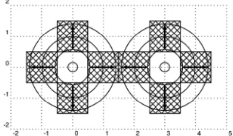
We also consider a bimodal density and conduct simultaneously local tests for modality based on the hypotheses (2.4) for the candidate modes x1 = (0,0) and x2 = (3,0). We conduct eight tests for the hypotheses (2.4) for a fixed bandwidthh=h0 = 0.5 with s1 =s5 =t1 = (1,0), s2 =s6 =t2 = (0,1),
s3=s7=t3= (−1,0),s4=s8=t4= (0,−1) andt5= (4,0),t6= (3,1), t7 = (2,0), t8 = (3,−1) and conclude thatf has a local maximum inx1 =
(0,0) whenever all hypotheses
Hsj,tj,h0
0,decr , j= 1, . . . ,4,
are rejected, that is
Fig 3. Illustration of the eight local tests for monotonicity used to create the tests (4.5)and
(4.6). The crosshatched squares display the support of the functionsFsj,tj,h
0,j= 1, . . . ,8, and the arrows the directional vectorssj,j= 1, . . . ,8.
and that f has a local maximum inx2= (3,0) whenever all hypotheses
Hsj,tj,h0
0,decr , j= 5, . . . ,8,
are rejected, that is
Tsnj,tj,h
0 > κ
j
n(α) for all j= 5, . . . ,8, (4.6)
where the quantileκj
n(α) is defined by (3.11). An illustration of the considered
scales is provided in Figure3. For the investigation of the approximation of the nominal level we consider a uniform distribution on the rectangle [−2.5,5.5]× [−2.5,2.5] for the density f. The scaling factor in the Laplace density is given byσ= 0.075. For power investigations we consider two bimodal densities given by a uniform mixture of a standard normal distribution and a N ((3,0), I) distribution (symmetric) and a uniform mixture of a N((0.0),1.2I) and a N ((3.2,0.1),0.8I) distribution (asymmetric). The results for the calibrated version of the test are given in Table7.
Symmetric Asymmetric n level powerx1 powerx2 powerx1 powerx2
500 5.3 34.6 33.0 23.6 48.5
1000 5.2 48.7 49.9 39.0 72.9
4000 4.2 84.4 81.7 76.1 97.1
Table 7
Simulated level and power of the tests (4.5)and (4.6)for a mode at the pointsx1= (0,0) andx2= (3,0), where the quantilesκj
n(α)are replaced by calibrated quantiles. The
random variablesZiin model (1.1)are given by a uniform mixture of a standard normal
distribution and aN((3,0), I)distribution (symmetric) and a uniform mixture of a
N((0.0),1.2I)and aN((3.2,0.1),0.8I)distribution (asymmetric).
We observe that in the symmetric case the test detects both modes with (roughly) the same power, whereas in the asymmetric case the mode with smaller variance (even though there is a slight misspecification of its position) is detected more often.
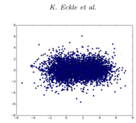
Fig 4. n = 4000 observations drawn from the convolution of a uniform mixture of a
N((0.0),1.2I)and aN((3.2,0.1),0.8I)distribution and a bivariate Laplace distribution with scale parameterσ= 0.5.
σ = 0.5 is given in Figure 4. Here, a look at the scatter plot does not give a hint on the number of modes of the distribution. However, the test (4.5), where the quantilesκjn(α) are replaced by calibrated quantiles, is still able to detect a mode at (0,0) in 48.4 percent of the repetitions and the test (4.6) with cal-ibrated quantiles detects a mode in (3,0) in 81.4 percent of the repetitions. The simulated level for the calibrated quantiles is 4.1.
4.3. Inference about local monotonicity of a multivariate density
The multiscale approach introduced in Section2can be used to obtain a graph-ical representation of the monotonicity behavior of a (bivariate) density. We construct a global map indicating monotonicity properties of the densityf by conducting the tests (3.10) for the hypotheses (2.2) for a fixed bandwidth of h = 0.5. The set of test locations Tt is defined as the set of vertices of an
equidistant grid in the square [−1,2]2 with width 1 and the set of test
direc-tions is given by Ts ={s1 =−s3 =
√
2−1(1,1), s2 =−s4 =√2−1(−1,1)}.
The tests (3.10) are conducted for every triple
(s, t, h0)∈Ts×Tt× {h0}.
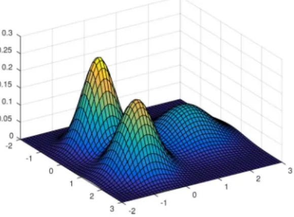
The scaling factor for the Laplace density in the convolution model (1.1) is given byσ= 0.075. We consider the tri-modal density with differently shaped modal regions displayed in Figure5.
Figure1in Section2provides the graphical representation of the monotonic-ity behavior of the densmonotonic-ity f. Here, each arrow at a location t in direction s displays a rejection of a hypothesis (2.2). The map indicates the existence of modes close to the points (−0.5,−0.5), (1.5,−0.5) and (0.5,1.5).
5. Proof of Theorem 3.1
Fig 5. The density of a (uniform) mixture of a N((−0.4,−0.57),0.2I),
N((1.5,−0.6),0.25I)andN((0.45,1.6),0.5I)distribution.
part of the proof we show the approximation (3.8). Finally we conclude by proving the boundedness of the limit distribution in the third part.
Throughout this section the symbolsandmean less or equal and greater or equal, respectively, up to a multiplicative constant independent of n and (s, t, h), and the symbol |as,t,h| |bs,t,h| means that |as,t,h/bs,t,h| is bounded
from above and below by positive constants.
5.1. Auxiliary results
We begin with some basic transformations of the deconvolution kernel Fs,t,h.
Recall that
Fs,t,h(.) =F−1
F(∂sφt,h)
F(fε)
(.) =h−d−1F−1
Rde−iy.x(∂sφ)((x−t)/h) dx F(fε)(y)
(.)
by definition of the kernelφt,h and the Fourier transform. A substitution in the
inner integral shows that
Fs,t,h(.) =h−1F−1
e−iy.tF(∂ sφ)(hy)
F(fε)(y)
(.). (5.1)
By the definition of the inverse Fourier transform and a substitution in the outer integral, we obtain
Fs,t,h(x) = h
−1
(2π)d
Rd
eix.y e−iy.tF(∂sφ)(hy)
F(fε)(y) dy=
h−d−1 (2π)d
Rd
eiy.x−ht F(∂sφ)(y)
F(fε)(y/h)dy. (5.2) Furthermore, as ∂sφ =
d
k=1sk∂ekφ, where ek, k = 1, . . . , d, denotes the kth unit vector of Rd, we have
F(∂sφ)(y) = d
k=1
whereidenotes the imaginary unit. The following lemma presents some imme-diate consequences of the Assumptions2and 3made in Section3.
Lemma 5.1. Let l∈ {1, . . . , d},m≥2 andm˜ =(d+ 1)/m. It holds 1. Ss=
Rd
1 +y2r/2F(∂sφ)(y)dy <∞uniformly with respect tos;
2.
Rd
∂m˜
∂ym˜ l
F(∂
sφ)(y)
F(fε)(y/h)
dyh−r.
Proof of Lemma 5.1. 1.: An application of Cauchy-Schwartz’s inequality yields for anyδ >0
Ss=
Rd
1 +y2r/2+(d+δ)/41 +y2−(d+δ)/4F(∂sφ)(y)dy
≤ Rd
1 +y2r+(d+δ)/2F(∂sφ)(y) 2
dy 1/21 +y2−(d+δ)/4L2(Rd).
By Assumption 3, there exists a constant δ > 0 such that the latter integral is bounded uniformly with respect to s. Hence, the assertion follows from the integrability of the function (1 +y2)−(d+δ)/2.
2.: By Leibniz’s rule we have
∂m˜
∂ym˜ l
F(∂
sφ)(y)
F(fε)(y/h)
˜ m k=0 ∂m˜−k
∂yml˜−kF(∂sφ)(y) ∂k
∂yk l
1 F(fε)(y/h)
.
Moreover, from Lemma7.2 it follows that
∂k
∂yk l
1 F(fε)(y/h)
(m1,...,mk)∈Mk
1
|F(fε)(y/h)|m1+...+mk+1
h−k
k
j=1
∂j
∂yljF(fε) (y/h)
mj,
whereMkis the set of allk-tuples of non-negative integers satisfying
k
j=1jmj=
k. Assumption2 in Section3 yields the estimates
∂j
∂yjlF(fε)(y)
1 +y2−(r+j)/2 and 1
|F(fε)(y)|
1 +y2r/2.
Thus, askj=1jmj =k for some (m1, . . . , mk)∈Mk, we find
∂k
∂yk l
1 F(fε)(y/h)
h−k
(m1,...,mk)∈Mk
1 +hy2(m1+...+mk+1)r/2
k
j=1
h−k
(m1,...,mk)∈Mk
1 +yh2(m1+...+mk+1)r/2
1 +yh2−(m1+...+mk)r/2−k/2
h−k1 +yh2(r−k)/2.
Hence,
∂m˜
∂ym˜ l
F(∂
sφ)(y)
F(fε)(y/h)
˜ m
k=0
h−k ∂
˜ m−k
∂yml˜−kF(∂sφ)(y)
1 +yh2(r−k)/2.
In the caser≥k, the claim is now a direct consequence of the estimate
h−k1 +yh2(r−k)/2h−r(1 +y2)(r−k)/2, similar arguments as given in proof of1.and Assumption3.
Ifr < kwe divide the integration area into the ballB1(0) and its complement.
For the integral
h−k
B1(0)C ∂m˜−k
∂ylm˜−kF(∂sφ)(y)
1 +hy2(r−k)/2dy
we haveh−k1 +y h2
(r−k)/2
h−r. Therefore, we can bound the integral over
the complement of the unit ball by the integral over Rd and proceed similarly to the first case. It remains to consider the integral over the ballB1(0). To this
end, notice that
h−k1 +yh2(r−k)/2≤h−ryr−k. Hence, by the boundedness of ∂m˜−k
∂yml˜−kF
(∂sφ) (which follows from the
compact-ness of the support ofφ) it remains to show that the integral
B1(0)
yr−kdy
1
0
ρd−1+r−kdρ
is bounded, where we used a polar coordinate transform to obtain the inequality. As k≤ (d+ 1)/2andr >0, the integral on the right hand side is obviously finite.
Part1 of the following lemma shows that the constantsV1, . . . , Vpdefined in
(3.6) are uniformly bounded from above and below.
Lemma 5.2. It holds
1. Fs,t,hL2(Rd)h−d/2−r−1;
2. Fs,t,hx−tL2(Rd)h−d/2−r;
3. Fs,t,hFs,t,hL1(Rd)(hh)−d/2−r−1;
4. Fs,t,hFs,t,hx−tx−tL1(Rd)(hh)−
Proof of Lemma 5.2. 1.: Using Plancherel’s theorem and the representation (5.1), we obtain
Fs,t,h2L2(Rd)h−2
e−iy.tF(∂ sφ)(h.)
F(fε)(.)
2
L2(Rd)=h −2
Rd
F(∂sφ)(hy)
F(fε)(y)
2dy.
(5.3) It now follows from Assumption2 and a substitution that
Fs,t,h2L2(Rd)h−d−2r−2
Rd
1 +y2)rF(∂sφ)(y) 2
dy,
and the latter integral is bounded by Assumption3 which concludes the proof of the upper bound.
For the lower bound we find from (5.3) and Assumption2 that
Fs,t,h2L2(Rd)h−2
Rd
1 +y2rF(∂sφ)(hy) 2
dy
h−d−2
Rd
1 +yh2rF(∂sφ)(y) 2
dy
h−d−2r−2
Ba(0)C
F(∂sφ)(y) 2
dy
for any constanta >0. Moreover,
Ba(0)C
F(∂sφ)(y) 2
dy=
Rd
F(∂sφ)(y) 2
dy−
Ba(0)
F(∂sφ)(y) 2
dy
∂sφ2L2(Rd)
for a sufficiently small radiusa by the integrability of|F(∂sφ)|2 (Assumption
3) and Plancherel’s theorem. Furthermore, the mapping s → ∂sφL2(Rd) is continuous such that by Assumption 3 ∂sφL2(Rd) ≥ c > 0 for a constant c that does not depend ons.
2.: The representation (5.2) and a substitution in the integral for the variable xshow
Fs,t,hx−t 2 L2(Rd)=
h−d
(2π)2d
Rd
x2
Rd
eiy.x F(∂sφ)(y) F(fε)(y/h)
dy2dx.
Asx2=x2
1+. . .+x2d, the differentiation rule for Fourier transforms yields
Fs,t,hx−t 2 L2(Rd)=
h−d
(2π)2d d k=1 Rd Rd eiy.x ∂
∂yk
F(∂
sφ)(y)
F(fε)(y/h)
dy2dx
=h−d
d
k=1
F−1 ∂
∂yk
F(∂
sφ)(y)
F(fε)(y/h)
h−d
d
k=1
∂
∂yk
F(∂
sφ)(y)
F(fε)(y/h)
2
L2(Rd),
where the last identity follows from Plancherel’s theorem. We now proceed sim-ilarly as in the proof of Lemma5.12.and note that
∂ ∂yk
F(∂sφ)(y)
F(fε)(y/h)
= ∂ ∂ykF
(∂sφ)(y)
1 F(fε)(y/h)
− F(∂sφ)(y)
F(fε)(y/h)
2
∂ ∂yk
F(fε)(y/h)
.
An application of the Assumptions2 and3shows
∂
∂ykF
(∂sφ)(y)
1 F(fε)(y/h)
2
L2(Rd)h −2r
Rd
∂
∂ykF
(∂sφ)(y) 2
1 +y2rdy
h−2r.
Moreover, by Assumption 2, we have
F(∂sφ)(y)
F(fε)(y/h)
2∂y∂
k
F(fε)(y/h) 2
L2(Rd)h −2
Rd
F(∂sφ)(y)2
1+hy2r−1dy.
This concludes the proof forr≥1. Forr <1 we split up the area of integration into the ball B1(0) and its complement and find the required result for the
integration over the complement using similar arguments as in the proof of Lemma 5.1 2. For the integral over the unit ball we also follow the line of arguments presented in the proof of Lemma 5.1 2. which yields the required result provided that the integral on the right hand side of the inequality
B1(0)
y2r−2dy
1
0
ρd−1+2r−2dρ
exists. This is the case for allr >0 ifd≥2 and allr > 1
2 in the cased= 1. 3. and 4.: These are direct consequences of H¨older’s inequality and1. resp.
2.
The following Lemma will be used in the second part of the proof of Theorem 3.1.
Lemma 5.3. For1≤j, k≤pandm≥2we have for the functionFj =Fsj,tj,h j
defined in (3.2)
Proof of Lemma 5.3. 1.: Using the representation (5.2) and Assumption2it follows that
|Fj(x)|h−jd−1
Rd
F(∂sjφ)(y) F(fε)(y/hj)
dy
h−jd−r−1
Rd
1 +y2r/2F(∂sjφ)(y)dy=h−jd−r−1Ssj. The claim follows from the uniform boundedness ofSsj shown in Lemma5.11.
2.: Using the representation (5.2), the boundedness of the density g and a substitution we get
Rd
Fj(x)m
g(x) dxh−jmd−m
Rd Rd eiy.
x−tj
hj F(∂sjφ)(y) F(fε)(y/hj)
dy
m
dx
=h−j(m−1)d−m
Rd Rd
eix.y F(∂sjφ)(y) F(fε)(y/hj)
dy
m
dx.
The proof will be completed showing the estimate
Rd Rd
eix.y F(∂sjφ)(y) F(fε)(y/hj)
dymdxh−jmr.
For this purpose we decompose the domain of integration for the variablexin two parts: the cube [−δ, δ]dfor someδ >0 and its complement. For the integral
with respect to the cube we use the upper bound Rd
F(∂sjφ)(y)
F(fε)(y/hj)
dy h−jr provided in the proof of1.which yields the required result.
For the integral with respect to ([−δ, δ]d)C note that
([−δ,δ]d)C
Rd
eix.y F(∂sjφ)(y) F(fε)(y/hj)
dymdx
≤ d k=1 d l=1 Ak,l Rd
eix.y F(∂sjφ)(y) F(fε)(y/hj)
dy
m
dx ,
where the setsAk,l are defined by
Ak,l=
x∈Rd| |xk|> δ,|xl| ≥ |xl|for alll=l
. Now ˜m=(d+ 1)/mfold integration by parts yields
Rd
eix.y F(∂sjφ)(y) F(fε)(y/hj)
dym= 1
|xl|mm˜
Rd eix.y ∂
˜ m
∂ym˜ l
F(∂
sjφ)(y) F(fε)(y/hj)
dym,
provided that ∂y∂m˜m˜
l
F(∂sjφ)(y)
F(fε)(y/hj)
∈ L1(Rd), which holds by Lemma 5.1 2. A
further application of Lemma5.12 shows that
Ak,l Rd
eix.y F(∂sjφ)(y) F(fε)(y/hj)
dymdxh−jmr
[−δ,δ]C
|xl|d−1
|xl|d+1
dxl,
5.2. Proof of the approximation (3.8)
For the consideration of the absolute values we introduce the set
T
n :=Tn∪ {(−s, t, h)|(s, t, h)∈Tn}=:{(sj, tj, hj)|j= 1, . . . ,2p}
and denote byA the set of all hyperrectangles inR2p of the form
A={w∈R2p|aj≤wj≤bj for all 1≤j≤2p}
for some −∞ ≤aj≤bj≤ ∞(1≤j≤2p).
We will show below in Section5.2.1that the random vectors
Xi= (Xi,1, . . . , Xi,2p)∈R2p, i= 1, . . . , n,
with
Xi,j=hd/2+r+1j
Fj(Yi)−E(Fj(Y1))
(i= 1, . . . , n, j= 1, . . . ,2p)
fulfill
sup
A∈A
P√1
n
n
i=1
Xi ∈A −P
1 √
n
n
i=1
Yi∈A
h−mind log 7
(n) n
1/6
+
h−d minlog
3
(n) n1−2/q
1/3
(5.4)
for anyq >0, whereY1, . . . , Yn are independent random vectors, Yi= (Yi,1 , . . . , Yi,2p )∼N (0,E(XiXi)), i= 1, . . . , n.
Note that we have
1
√
n
n
i=1
Yi∼N(0,E(X1X1)),
where
E(X1X1) =
(hjhk)d/2+r+1
E(Fj(Y1)Fk(Y1))−E(Fj(Y1))E(Fk(Y1))
1≤j,k≤2p,
as the random variablesX1, . . . , Xn are i.i.d. andY1, . . . , Yn are independent.
Introduce a Gaussian process ( ˜B(Φ))Φ∈L∞(Rd)indexed byL∞(Rd) as a pro-cess whose mean and covariance functions are 0 and
Rd
Φ1(x)Φ2(x)g(x) dx−
Rd
Φ1(x)g(x) dx
Rd
Φ2(x)g(x) dx, (5.5)
respectively. Hence, there exists a version of ˜B(Φ) such that 1
√
n
n
i=1
Yi =hd/2+r+11 B(F˜ 1), . . . , hd/2+r+12p B(F˜ 2p)
.