The Factory and the Beehive. III. PTFEB132.707
+
19.810, A Low-mass Eclipsing Binary
in Praesepe Observed by PTF and
K2
Adam L. Kraus1 , Stephanie T. Douglas2 , Andrew W. Mann1,11 , Marcel A. Agüeros2 , Nicholas M. Law3 , Kevin R. Covey4 , Gregory A. Feiden5 , Aaron C. Rizzuto1 , Andrew W. Howard6 , Howard Isaacson7 , Eric Gaidos8,
Guillermo Torres9 , and Gaspar Bakos10,12 1
Department of Astronomy, The University of Texas at Austin, Austin, TX 78712, USA
2
Columbia University, Department of Astronomy, 550 West 120th Street, New York, NY 10027, USA
3
Department of Physics and Astronomy, University of North Carolina, Chapel Hill, NC 27599, USA
4
Western Washington University, Department of Physics & Astronomy, Bellingham, WA 98225, USA
5
Department of Physics, University of North Georgia, Dahlonega, GA 30597, USA
6
California Institute of Technology, 1200 E. California Boulevard, Pasadena, CA 91125, USA
7
University of California, Berkeley, Berkeley, CA 94720, USA
8
Department of Geology and Geophysics, University of Hawaii at Manoa, Honolulu, HI 96822, USA
9
Harvard-Smithsonian Center for Astrophysics, 60 Garden Street, Cambridge, MA 02138, USA
10
Department of Astrophysical Sciences, Princeton University, Princeton, NJ 08544, USA
Received 2017 March 23; revised 2017 June 19; accepted 2017 June 28; published 2017 August 11
Abstract
Theoretical models of stars constitute the fundamental bedrock upon which much of astrophysics is built, but large swaths of model parameter space remain uncalibrated by observations. The best calibrators are eclipsing binaries in clusters, allowing measurement of masses, radii, luminosities, and temperatures for stars of known metallicity and age. We present the discovery and detailed characterization of PTFEB132.707+19.810, aP=6.0 day eclipsing binary in the Praesepe cluster(τ∼600–800Myr;[Fe/H]=0.14±0.04). The system contains two late-type stars (SpTP=M3.5±0.2; SpTS=M4.3±0.7) with precise masses (Mp=0.39530.0020Me; Ms=0.2098
0.0014Me) and radii (Rp =0.3630.008Re; Rs =0.2720.012Re). Neither star meets the predictions of
stellar evolutionary models. The primary has the expected radius but is cooler and less luminous, while the secondary has the expected luminosity but is cooler and substantially larger(by 20%). The system is not tidally locked or circularized. Exploiting a fortuitous 4:5 commensurability betweenPorbandProt,prim, we demonstrate that
fitting errors from the unknown spot configuration only change the inferred radii by1%–2%. We also analyze subsets of data to test the robustness of radius measurements; the radius sum is more robust to systematic errors and preferable for model comparisons. We also test plausible changes in limb darkening and find corresponding uncertainties of∼1%. Finally, we validate our pipeline using extant data for GU Boo,finding that our independent results match previous radii to within the mutual uncertainties(2%–3%). We therefore suggest that the substantial discrepancies are astrophysical; since they are larger than those for old field stars, they may be tied to the intermediate age of PTFEB132.707+19.810.
Key words:binaries: eclipsing –stars: evolution–stars: fundamental parameters –stars: individual (PTFEB132.707+19.810)–stars: low-mass–starspots
Supporting material:machine-readable tables
1. Introduction
The fundamental properties of stars establish the foundation for much of astrophysics, and uncertainties in model-derived stellar properties propagate into systematic uncertainties in the initial mass function (Bastian et al. 2010), the age-activity-rotation relation (Agüeros et al.2011; Douglas et al.2016; Rebull et al.2016), and exoplanet masses and radii (e.g., Gaidos & Mann 2012; Bastien et al. 2014). The relations between mass, radius, luminosity, temperature, and metallicity, or subsets thereof, have traditionally been calibrated with observations of the Sun, stellar populations, or binary systems. However, these calibrations remain sparse and observationally expensive for low-mass stars due to their intrinsically low luminosities. The past 15 years have seen benchmark calibrations for the relations for mass–luminosity(with visual binaries; Delfosse et al. 2000), luminosity–temperature– radius(with long-baseline interferometry; Boyajian et al.2012), and
luminosity–temperature–metallicity(with spectroscopy; Mann et al. 2015), typically with a scatter of ∼5% for mass or radius measurements.
Direct measurements of the mass–radius relation are typically derived from studies offield eclipsing binary systems (e.g., Torres et al.2010), for which the orbit yields masses and the eclipses yield radii. Eclipsing binaries can yield mass and radius measurements with formal uncertainties of 1%, surpassing the precision offered by visual binaries or long-baseline interferometry, but due to their faintness only a modest number of systems with low-mass components(Mp0.7M)
have been discovered and characterized. The systems dis-covered to date have suggested that models and observations are discrepant in at least some cases, with models predicting radii that are up to 10% too low for a given mass(e.g., López-Morales2007; Torres et al.2010). This problem has been seen for solar-type stars for several decades (e.g., Popper 1997; Torres et al.2006; Torres et al.2008; Clausen et al.2009). The most recent compilations by Dittmann et al. (2017) and © 2017. The American Astronomical Society. All rights reserved.
11
Hubble Fellow.
12
Iglesias-Marzoa et al.(2017)show that this scatter exists for the entire mass range 0.2M<M<1.0M; some stellar radii match model predictions, but most stars are larger.
It remains unclear whether the radius discrepancy results from physics common to all low-mass stellar interiors(e.g., requiring extra opacities or modified treatments of convection, metallicity, or magnetic fields; Feiden & Chaboyer 2014a, 2014b) or a systematic effect specific to the short-period binary systems that are most likely to eclipse. These short-period systems are often tidally locked to rapid rotation periods that sustain high levels of magnetic activity, possibly leading to larger radii than are predicted by nonmagnetic stellar models (Chabrier et al. 2007; Morales et al. 2009; Kraus et al. 2011; Mullan & MacDonald 2001). However, even some very long-period systems are larger than models would predict(Irwin et al.2011).
Eclipsing binaries in star clusters offer even stronger tests, allowing measurement of the masses, radii, luminosities, temperatures, metallicities, and ages of the component stars, but those systems have been rare to date. PTFEB132.707
+19.810—also AD 3814 (Adams et al. 2002), 2MASS J08504984+1948364(Cutri et al.2003), and EPIC 211972086 (Huber et al.2016)—wasfirst suggested as a candidate member of the Praesepe open cluster by Adams et al. (2002), who assessed a membership probability of 48.4% based on its 2MASS/POSS colors and proper motion. The membership probability was subsequently revised upward to 97.9% by Kraus & Hillenbrand(2007)based on its 2MASS/USNO-B1.0/SDSS photometry and proper motion, while Boudreault et al. (2012) assessed a membership probability of 86% based on UKIDSS photometry and proper motion. Kraus & Hillenbrand (2007) estimated the spectral type to be M3.4 based on the broadband optical/NIR SED, and West et al. (2011)analyzed the SDSS spectrum to estimate a spectral type of M5.
PTFEB132.707+19.810 was closely inspected by the Palomar Transient Factory(PTF)Open Cluster Survey(POCS) due to its likely Praesepe membership and its nature as a mid-M dwarf. Agüeros et al. (2011)measured a rotation period of
Prot=7.43days based on clear periodic brightness variations. As we describe below, PTFEB132.707+19.810 also was identified to be an eclipsing binary with an orbital period of
Porb=6.0days that has not locked its stars into synchronous rotation. The star has otherwise remained anonymous in the literature until this year, when its eclipsing nature was recognized by others studying K2 data in Praesepe (Douglas et al.2017; Gillen et al.2017; Rebull et al.2017). In this paper, we analyze our discovery light curve from PTF, follow-up spectroscopic observations, and the newly released K2 light curve of PTFEB132.707+19.810 in order to measure the stellar properties of this mid-M-type eclipsing binary system and test the predictions of stellar evolutionary models. In Section2, we describe our observations of this system, and in Section 3, we describe the analysis used to interpret those observations. We summarize the resulting properties for the system in Section 4, as well as testing the robustness of our results. Finally, in Section5, we discuss the implications of our results for the current generation of stellar evolutionary models.
2. Observations
2.1. PTF Photometry
The PTF uses wide-field photometric observations from the robotic 48 inch Samuel Oschin Telescope (hereafter P48), a
Schmidt camera with a wide focal plane. When PTFEB132.707
+19.810 was observed in 2010 and 2011, P48 was equipped with the CFH12K mosaic camera that had been installed on the Canada–France–Hawaii Telescope (Rahmer et al. 2008). The camera covered a totalfield of 8 deg2(with 7.26 deg2of useful area, since one chip was nonfunctional), sampled with a pixel scale of 1″. The observations that we report were taken in the standard PTF observing mode, which uses 60 s integrations through a MouldRfilter, yielding photometry for all stars down to mR ~20mag (Ofek et al. 2012). The Praesepe field was typically observed 1–2 times per night as part of the POCS campaign(Agüeros et al. 2011), but it was also observed at a more rapid cadence(every 15 minutes, yielding 15–30 images per night) on some nights as part of the PTF/M-dwarfs campaign(Law et al. 2011; Law et al.2012). PTFEB132.707
+19.810 was observed 622 times over the course of these two PTF programs.
The construction and analysis of light curves for the POCS and PTF/M dwarfs programs were described in more detail by Law et al.(2009,2012)and Agüeros et al. (2011). To briefly summarize, the images werefirst calibrated to correct for cross talk, perform bias/overscan subtraction, and divide by a contemporaneous superflat. The data were then processed with SExtractor to measure source photometry, and sources were matched across all epochs. The photometric zero points for each epoch were initially estimated based on SDSS photometry for bright stars in the field, and then the zero point for each epoch was optimized to minimize the median photometric variability of all remaining sources, rejecting apparently variable sources. The pipeline typically achieved a photometric stability of 3–5 mmag over periods of months; the photometric uncertainties for all observations of PTFEB132.707+19.810 were limited by photon noise.
PTFEB132.707+19.810 was identified as a candidate eclipsing binary system using a Box Least Squares algorithm (Kovács et al.2002)that phased the light curves to all possible periods and searched for a transit- or eclipse-like signature. The identification of eclipses was then visually confirmed.
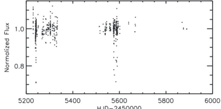
We list all of the photometric measurements for PTFEB132.707+19.810 in Table1; in Figure1, we show the light curve spanning three observing seasons.
2.2. K2 Photometry
PTFEB132.707+19.810 was observed as EPIC 211972086 by theKeplerspacecraft during Campaign 5 of its repurposed
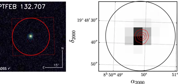
K2mission(Howell et al.2014), for which it was proposed as a target by eight proposals, including ours (GO5095; PI: Agüeros). K2 observed PTFEB132.707+19.810 in long-cadence mode (tint=29.4minutes) for 73.9 continuous days spanning 2015 April 27–July 10, yielding 3402 exposures of the 9×8 pixel postage stamp centered on the target. We show the postage stamp superimposed on SDSS images of thefield and one frame from the postage stamp in Figure2. TheK2data were downloaded from the Mikulski Archive for Space Telescopes as target pixelfiles, which contain the barycentric corrected observation times, theflux measured in each pixel at each epoch, and quality flags. We omitted the 15 exposures where the qualityflag is not zero.
being sampled across the detector pixels (and their response function)differently over time(Vanderburg & Johnson2014). The light curve also shows visually obvious sinusoidal periodicity with a period of Prot~7.5days and amplitude
±3%, as well as clear primary and secondary eclipses with a periodicity ofPorb~6.0days. The primary starflux contributed
∼75% of the total opticalflux(Section2.4), so the origin of the sinusoidal periodicity was most likely rotational modulation due to spots on the primary. We prepared the light curve for eclipsefitting by using the methods described by Douglas et al. (2016) to measure photometry and rectify the stellar and instrumental variability.
We began by computing and subtracting the background in each exposure using an iterative 3σ clipped median and then measured the flux of PTFEB132.707+19.810 through a soft-edged circular aperture with a radius of 4 pixels, yielding a raw light curve. The aperture was centered on the photocenter in each exposure, so it tracked the drift of the target. We then detrended the long-timescale variability using the Python routine supersmoother13 (Friedman 1984; Vanderplas & Willmer2015)with a high bass-enhancement value(a=10). We measured the period of the sinusoidal variability using the Lomb–Scargle function in the Python package gatspy
(Vanderplas et al.2016), an implementation of the Fast Fourier Transform (FFT)-based algorithm from Press & Rybicki (1989). We computed the periodogram power for 3´104 periods spanning 0.1–70.8 days and established false-alarm probabilities using nonparametric bootstrap resampling to generate 103 simulated light curves. To divide out the sinusoidal variability, we folded the light curve on the most likely period and used supersmoother to produce a smoothed periodic light curve. After iterating this procedure six times to
remove stellar variability, we next measured the time-dependent flat field at each epoch by calculating the median
flux for the 21 other epochs with the closest centroid positions (in detector coordinates). We then returned to the raw light curve and first applied the flat-field correction, then fit and rectified the stellar variability. Finally, we rectified the remaining low-order power in the light curve by dividing the
flux at each epoch by the median of all other noneclipsefluxes observed within±12 hr.
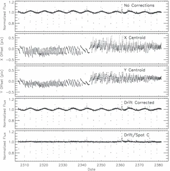
We show the stages of this process in Figure3and present the resulting normalized fluxes in Table 2. We found a final best-fit rotational period (most likely for the primary) of
Prot=7.46days, which is nearly identical to the period of
P=7.43 days measured by Agüeros et al. (2011). We also repeated our analysis for the same light curve extracted by K2 Systematics Correction(K2SC; Aigrain et al.2016)and found a period of P=7.49 days. The uncertainties in rotational periods are dominated by systematic effects due to evolution of the(unmeasurable)spot configuration, but different surveys of rotation in open clusters have typically yielded values that agree to within2%–3%(e.g., Douglas et al.2016), so these measurements are statistically indistinguishable. The light curve also contains numerous flares; one primary eclipse (at epoch 2361)and one secondary eclipse(at epoch 2364)were contaminated byflares, so we have omitted those observations from our light-curvefits.
2.3. Archival Photometry
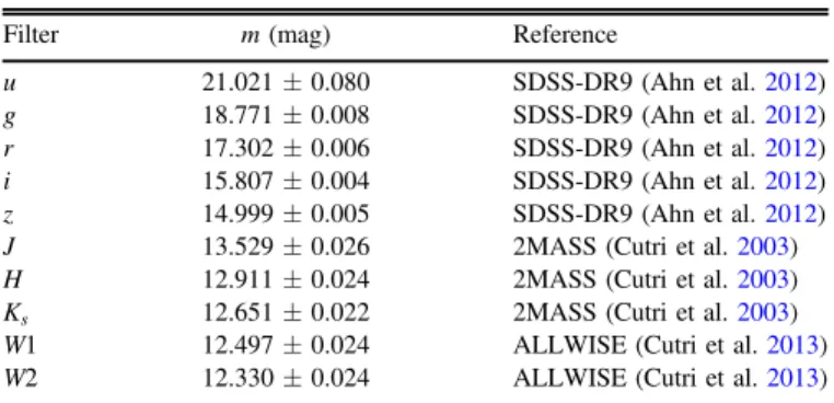
As part of our analysis to compute a bolometricflux for this system, we also have compiled all of the available( component-unresolved)photometry in all-sky surveys. As we summarize in Table3, we have used photometry from SDSS-DR9(u,g,r,
i,z; Ahn et al.2012), 2MASS(J,H,Ks; Cutri et al.2003), and AllWISE(W1,W2, W3; Cutri et al.2013).
2.4. Keck/HIRES High-resolution Spectroscopy and Radial
Velocities
After our discovery of eclipses in this system in 2010, we began a spectroscopic monitoring campaign to measure radial velocities (RVs) for the components. We obtained 20 high-dispersion spectra for the system using Keck I and the HIRES spectrograph (Vogt et al.1994), which is a single-slit echelle spectrograph permanently mounted on the Nasmyth platform. Ten spectra were obtained using classical observing on three nights. These observations were performed using the red channel and C1 decker and spanned a wavelength range of
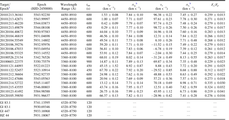
Table 1 PTF Photometry
Epoch Phase R sR
(HJD-2450000) (mag) (mag)
5229.7300 0.6192 16.987 0.060
5229.7420 0.6212 16.910 0.038
5229.7430 0.6214 16.951 0.042
5229.7490 0.6224 17.035 0.044
5229.7500 0.6226 16.923 0.048
5229.7550 0.6234 16.969 0.050
5229.7570 0.6237 17.015 0.060
5229.7840 0.6282 16.919 0.052
5229.7980 0.6305 16.992 0.054
5229.8030 0.6314 17.057 0.043
5229.8050 0.6317 16.941 0.049
5229.8240 0.6349 17.029 0.045
5229.8260 0.6352 16.996 0.044
5239.7080 0.2779 17.070 0.025
5239.7100 0.2782 17.100 0.024
5239.7210 0.2800 17.052 0.024
5239.7230 0.2804 17.083 0.027
5239.7330 0.2820 16.985 0.037
5239.7710 0.2884 17.075 0.049
5239.7730 0.2887 17.087 0.062
5239.8040 0.2938 17.040 0.024
(This table is available in its entirety in machine-readable form.)
Figure 1.PTF aperture photometry results for the Praesepe eclipsing binary PTFEB132.707+19.810, with fluxes normalized to the median value
(mR=17.03 mag).
13
4500–8900 Å, yielding a spectral resolution of R~48,000. We processed our HIRES data using the standard pipeline MAKEE14, which automatically extracts, flat-fields, and wavelength-calibrates spectra taken in most standard HIRES configurations. Ten additional spectra were obtained in a queue mode via collaboration with the California Planet Search(CPS) on nine nights, so as to obtain broader phase coverage for the system. These observations were performed using the red channel and C2 decker and spanned a wavelength range of 3400–8100 Å, also yielding R∼48,000. These data were extracted using the standard CPS pipeline(Howard et al.2010). In both cases, we refined the wavelength solution by cross correlating the 7600 Å O2telluric absorption band against that
of the spectrophotometric standard star HZ 44 (Massey et al. 1988).
Our analysis of the HIRES data to measure RVs is identical to the methods described in Kraus et al. (2011,2014, 2015). For each spectrum, we measured the broadening function (Rucinski1999)15with respect to three Keck/HIRES observa-tions of two standard stars with similar temperature and metallicity: one observation of Gl 447 and two separate observations of Gl 83.1 on different nights. The broadening function is a better representation of the rotational broadening convolution than a cross correlation, since it is less subject to “peak pulling”and produces aflatter continuum. We fit each broadening function with two Gaussian functions to determine the absolute primary- and secondary-star RVs (vpand vs), the
standard deviations of the line width due to rotation and instrumental resolution(svpandsvs), and the averageflux ratio
across all well-fit orders(which is estimated from the ratio of areas for the two peaks of the broadening function). We list these measurements in Table4.
In Table5, we list the equivalent widths of Hαemission for those epochs where the lines from the two stars were fully resolved (i.e., within D <f 0.1 of orbital quadrature). The equivalent widths are measured with respect to the continuum of the full composite spectrum, but individual stellar values can be determined from theflux ratio of the spectra(which is nearly constant across the entire wavelength range of the HIRES spectra). We also show narrow wavelength ranges around Hα in each spectrum in Figure 4. As can be seen, while the Hα emission of the primary is clearly evident, the emission from the secondary is weaker and can only be measured in aggregate by measuring the excessflux over the continuum within±1 Å of the expected line center.
To estimatevsin( )i fromsv, we artificially broadened each of
our template spectra using the IDL task lsf_rotate (Gray 1992; Hubeny & Lanz2011)using a range of rotational velocities and then computed each artificial spectrum’s broadening function using the corresponding original template. This process yielded a relation between vsin( )i and sv that is appropriate for any
spectrum observed with Keck/HIRES at this spectral resolution and can be applied to thesvvalues that emerge from the Gaussian
function that wefit to each component’s broadening function peak in our analysis. Using the 10 spectra with the lowest inter-order scatter ofsv, wefind that the mean and standard error of the line
broadening for each star are sv p, =7.780.02kms−1and 7.55 0.05
v s,
s = kms−1, which correspond to vpsin( )i =
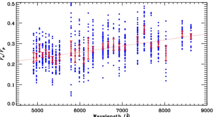
2.60.6kms−1andvssin( )i <2.0kms−1, respectively. In Figure 5, we show the flux ratio measured for the two stars, as computed from the broadening functions for each order of each spectrum, as well as the mean and standard error for each order after applying a 2σ clip. The flux ratio should depend on wavelength for two stars with unequal temperatures, and wefind that there is a positive linear correlation with slope
a=2.97´10-5Å−1
. As we discuss below, the points constituting this wavelength-dependent relation provide an
Figure 2. Left: SDSSrpostage stamp of PTFEB132.707+19.810(FOV=60″, north=up)showing theK2postage stamp(red box)and our adopted 4pixel photometric aperture(red circle). The image is shown in a square-root stretch using the CubeHelix color palette(Green2011). There are no nearby sources on the postage stamp or anywhere in the image. PTFEB132.707+19.810 has not been observed with adaptive optics, so there are no limits on closer companions, though the absence of a third set of spectral lines in our spectra suggests that there are no additional objects withinD <R 2. Right: postage stamp of PTFEB132.707+19.810 that was downloaded as part ofK2’s Campaign 5, showing the co-added sum of all frames. The black circle shows the 4pixel photometric aperture used in our analysis. The red contours show theflux distribution of the SDSS image.
14
http://www.astro.caltech.edu/~tb/makee/
15
important constraint in deconvolving the combined-light spectra taken with the Supernova Integral Field Spectrograph (SNIFS) and SpeX.
2.5. Intermediate-resolution Spectroscopy
We obtained an optical spectrum of PTFEB132.707+19.810 on 2016 April 3 with SNIFS(Aldering et al.2002; Lantz et al. 2004) on the University of Hawai’i 2.2 m telescope on Maunakea. SNIFS covers 3200–9700 Å simultaneously with a resolution ofR~700andR~1000in the blue(3200–5200 Å) and red(5100–9700 Å)channels, respectively. We observed with a total integration time of3´1200=3600 s, yielding a signal-to-noise ratio(S/N)=100 per resolving element atl=6500 Å. We also observed spectrophotometric standards forflux calibra-tion and obtained a ThAr arc before or after each observacalibra-tion for wavelength calibration. Bias subtraction, flat fielding, dark correction, cosmic-ray rejection, construction of data cubes, and extraction of thefinal spectrum were performed as described in detail by Aldering et al.(2002). Theflux calibration was derived from the combination of the spectrophotometric standards and a
model of the atmospheric absorption above Maunakea as described by Mann et al.(2015).
We obtained a NIR spectrum of PTFEB132.707+19.810 on 2016 April 5 with the SpeX spectrograph(Rayner et al.2003) on the NASA Infrared Telescope Facility on Maunakea. SpeX observations were taken in the short cross-dispersed mode using the 0 3×15″slit, yielding simultaneous coverage from 0.8 to 2.4μm at a resolution of R~2000. The target was observed in an AB nod pattern to allow for sky subtraction. We took a total of 34 exposures totaling 4080 s, yielding S/N=100 per resolving element atl=2.2μm. Spectra were extracted using the SpeXTool package (Cushing et al.2004), which performs flat fielding, wavelength calibration, sky subtraction, and extraction of the final spectrum. Exposures were combined using the IDL routinexcombspec. Telluric lines were corrected using a spectrum of the A-type star HD 68703, which was observed immediately before the target with a difference of<0.1airmass, and the correction was computed and applied using thextellcorpackage(Vacca et al.2003).
Following the method outlined by Mann et al. (2015), we combined and absolutely flux calibrated the optical and NIR spectra using published photometry(Section2.5)with thefilter
Figure 3.K2aperture photometry results for the Praesepe eclipsing binary PTFEB132.707+19.810(EPIC 211972086). Time is specified in units of BJD-2454833, the standard time system forK2. First panel: normalized light curve extracted from aperture photometry, without any subsequent detrending. Second and third panels: X and Y centroid positions, in pixels, as a function of time. The 6 hr interval between thrusterfirings(which reset the telescope position)is evident in the positions, and the position information can be used to detrendflux variations as the target moves across the detector. Fourth panel: normalized light curve after correctingfl
profiles and zero points provided by Fukugita et al.(1996)and Mann & von Braun(2015).
3. Analysis
3.1. Atmospheric Properties and Radius Ratio from Spectra
We initially analyzed the system as a single, unresolved object. Following Mann et al.(2015), we combined the optical and NIR spectra (Section2.5), which we simultaneously flux calibrated using available photometric measurements (Section2.3)and the appropriate zero points and filter profiles (Cohen et al. 2003; Mann & von Braun 2015). We filled in missing regions of the spectrum and areas of high telluric contamination with the best-fit BT-SETTL atmospheric model (Allard et al. 2011). Once combined and calibrated, we dereddened the spectrum byE B( -V)=0.0270.004mag (Taylor2006)and then integrated over wavelength to compute the bolometricflux. Accounting for errors in theflux calibration, photometry, photometric zero points, and reddening, we derived a final bolometric flux of Fbol=(1.750.06)´ 10-11erg cm−2s−1. To compute the bolometric luminosity, we
adopted the distanced =1826pc(van Leeuwen2009)and foundLbol=0.01800.0010L.
The luminosities and temperatures of the individual stars are subject to a strong joint constraint from the unresolved magnitudes and spectra of the PTFEB132.707+19.810 system when combined with Praesepe’s known distance and red-dening. However, the colors and molecular absorption bands of M dwarfs vary smoothly and monotonically with temperature, so the same unresolved features are degenerately consistent with a range of plausible temperature and luminosity combinations. To determine nondegenerate temperatures and luminosities for each star, we therefore must also use the wavelength-dependent flux ratio inferred from our Keck/ HIRES observations(Section2.4; Figure5). The same analysis also provides a useful prior for our light-curve analysis. While eclipse light curves strongly constrain the sum of the stellar radii, they offer a weaker constraint on the ratio of the radii; a very similar light curve results from making one star larger and the other smaller and then optimizing the inclination to match. We have combined all of these data in a simultaneous fit against a library of empirical, flux-calibrated spectra. We adopted these library spectra from the large sample of nearby M dwarfs considered by Mann et al.(2015). These stars have high-quality measurements of their distancesd(from parallax), metallicities [Fe/H] (from spectra; Mann et al. 2013b), bolometricfluxesFbol (from spectra and panchromatic
broad-band photometry), and effective temperaturesTeff(from colors
and spectra, using a relation bootstrapped from stars with interferometric radius measurements; Boyajian et al. 2012; Mann et al.2013a). Using the Stefan–Boltzmann law and the known values ofd, Fbol, andTeff, we computed the radius of
each library star. We then combined it with the absolutefl ux-calibrated spectra to compute the emergent spectralflux density or surface brightness (Sl, in erg s−1cm−2Å−1) of the star, as well as the emergent spectral flux densities when averaged across each order of our HIRES spectra and when convolved with theKeplerand PTF bandpasses(SKepand SPTF).
After constructing this library, we then combined all possible pairs of templates with metallicities consistent with Praesepe ([Fe/H]=0.14±0.04; Taylor2006)and compared them to the absolutely calibrated unresolved spectrum (Section 2.5) and spectrally resolved HIRES flux ratios (Section 2.4) of the PTFEB132.707+19.810 A+B system. For each system, our analysis explored the range of allowed totalflux ratios(and hence radius and surface brightness ratios)that was consistent with the Keck/HIRES and SNIFS+SpeX results. For each possible combination, we solved for the component stellar radii that would best reproduce the absolute and relative flux measurements of PTFEB132.707+19.810 and adjusted the total brightness of the template spectra as appropriate. From the scaled spectra, we
computed the radius ratio R
R
s
p
( )
,Keplerbandpassflux ratio SS s Kep p Kep , ,
( )
, PTF bandpassflux ratio SS
s
p ,PTF
,PTF
( )
, andc2 of thefit as dependent variables. We show one example of this fitting procedure in Figure 6, representing the sum of templates that produce the bestfit.Thec2goodness-of-fit statistic is poorly defined for spectra that have a very large number of wavelength channels and errors that are dominated by the covariance between channels. These covariances can be integrated into the analysis using tools such as Starfish(Czekala et al.2015), but the run time for a large spectral library would be infeasibly long. To avoid
Table 2
K2Photometry
Epoch Phase F sF
(HJD-2450000) (Normalized) (Normalized)
7139.6011 0.0981 0.995 0.008
7139.6215 0.1015 0.999 0.007
7139.6419 0.1049 0.995 0.007
7139.6624 0.1083 0.994 0.007
7139.6828 0.1117 1.002 0.007
7139.7032 0.1151 0.998 0.007
7139.7236 0.1185 1.001 0.007
7139.7441 0.1219 1.015 0.007
7139.7645 0.1253 1.018 0.007
7139.7849 0.1287 1.004 0.007
7139.8054 0.1321 0.996 0.007
7139.8258 0.1355 0.977 0.007
7139.8462 0.1389 0.860 0.007
7139.8667 0.1423 0.799 0.007
7139.8871 0.1456 0.882 0.007
7139.9075 0.1490 0.993 0.007
7139.9280 0.1524 1.000 0.007
7139.9484 0.1558 0.998 0.007
7139.9688 0.1592 0.995 0.007
7139.9893 0.1626 1.000 0.007
7140.0097 0.1660 0.998 0.007
(This table is available in its entirety in machine-readable form.)
Table 3 System Photometry
Filter m(mag) Reference
u 21.021±0.080 SDSS-DR9(Ahn et al.2012)
g 18.771±0.008 SDSS-DR9(Ahn et al.2012)
r 17.302±0.006 SDSS-DR9(Ahn et al.2012)
i 15.807±0.004 SDSS-DR9(Ahn et al.2012)
z 14.999±0.005 SDSS-DR9(Ahn et al.2012)
J 13.529±0.026 2MASS(Cutri et al.2003)
H 12.911±0.024 2MASS(Cutri et al.2003)
Ks 12.651±0.022 2MASS(Cutri et al.2003)
W1 12.497±0.024 ALLWISE(Cutri et al.2013)
having thefit dominated by the spatially unresolved spectra, we instead weighted the finalc2 contributions of the unresolved spectrum to equal twice the combined contributions of the HIRESflux ratio(with 27degrees of freedom)and rescaled all of thec2 values so that the best-fit value would havec2=1
n .
Adjusting the weighting by a factor of 5 did not change the results in a significant way.
The result of this analysis is a posterior distribution for the radius ratio R
R
s
p
, the Kepler bandpass (Kp) surface brightness
ratio S S s Kep p Kep , ,
, and the PTF bandpass(MouldR)surface brightness
ratio S S s p ,PTF ,PTF
. There are several confounding variables (such as
metallicity, stellar age, and spot coverage), and even small errors in the flux calibration can lead to significant spectral mismatch across many channels, so there is not a smoothc2 hypersurface within this three-dimensional space. Adjacent points differ significantly in c2. We instead constructed the joint posterior using the 9276 template pairs with a goodness of
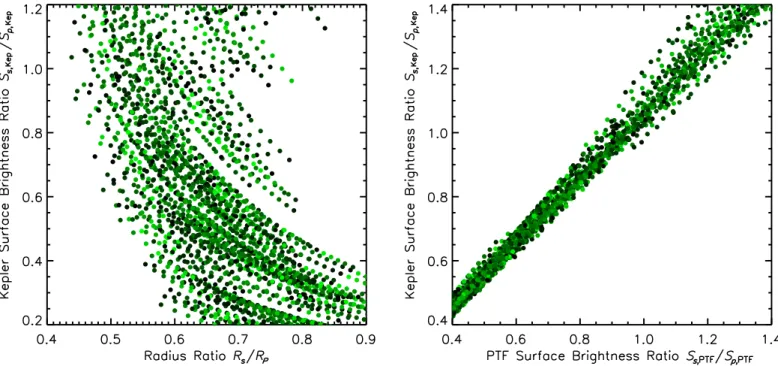
fitcn2<4 (chosen to yield visually acceptable matches to the spectra), taking the density of fit results in the three-dimensional space as a measure of the posterior probability density. To avoid establishing a prior that goes to zero outside of the distribution of points, but instead declines smoothly away from this locus, we defined the density at a given location in parameter space by convolving each discrete point with a 3D Gaussian blurring function, with s=0.05 on all axes. We verified that the shape of this posterior does not change significantly forc2 cuts or different values ofσ, even extending to much poorer fits (c2n~10) where the spectral mismatch is visually obvious. In Figure7, we show the distribution of 9276 points that defines our posterior distribution forR
R s p ,S S s Kep p Kep , ,
, andS
S s p ,PTF ,PTF . In addition to computing a spectroscopic prior for our Markov chain–Monte Carlo (MCMC) orbit analysis, we also used the same template library and fitting scheme to estimate posteriors for the best-fit temperatures, spectral types, and bolometric fluxes for the components of PTFEB132.707
Table 4 Keck I/HIRES RVs
Target/ Epoch Wavelength tint vp svp
b vs
vs s b
F Fs p
Epocha (HJD-2450000) Range(Å) (s) (kms−1) (kms−1) (kms−1) (kms−1)
20101213.36161 5543.92230 4450–8910 600 1.53±0.08 7.84±0.10 96.38±0.22 7.45±0.27 0.259±0.013 20101213.42871 5543.99997 4450–8910 600 1.00±0.07 7.71±0.07 97.61±0.23 7.78±0.30 0.271±0.013 20101213.46220 5544.03873 4450–8910 600 0.42±0.09 7.79±0.07 97.74±0.23 7.48±0.24 0.279±0.011 20101213.49879 5544.08108 4450–8910 450 0.29±0.11 7.77±0.10 98.72±0.26 7.50±0.26 0.274±0.017 20120104.40672 5930.97583 4450–8910 600 44.04±0.10 7.77±0.09 16.96±0.18 7.60±0.16 0.283±0.013 20120104.46819 5931.04698 4450–8910 900 46.56±0.10 7.84±0.08 12.31±0.14 7.84±0.22 0.266±0.012 20120104.55549 5931.14802 4450–8910 600 49.54±0.11 7.73±0.08 6.10±0.26 7.71±0.48 0.268±0.012 20120106.39276 5932.95976 4450–8910 600 59.20±0.11 7.71±0.10 −11.52±0.15 7.49±0.22 0.279±0.011 20120106.47033 5933.04954 4450–8910 1200 56.81±0.10 7.83±0.06 −6.78±0.19 7.39±0.12 0.261±0.012 20120106.55325 5933.14552 4450–8910 600 53.91±0.12 7.84±0.07 −2.04±0.30 7.44±0.25 0.279±0.014 20100526.23134 5342.76526 3360–8100 900 68.01±0.19 8.02±0.14 −31.24±0.49 8.13±0.55 0.263±0.017 20100603.22375 5350.75579 3360–8100 900 14.87±0.11 7.89±0.13 69.87±0.34 7.35±0.48 0.229±0.023 20101121.44093 5522.01223 3360–8100 450 45.15±1.52 8.92±0.87 8.88±0.43 7.72±0.20 0.291±0.025 20101122.52457 5523.10914 3360–8100 450 67.70±0.22 7.92±0.20 −29.52±0.85 8.68±0.88 0.312±0.027 20101212.36604 5542.92735 3360–8100 600 24.98±0.12 7.62±0.16 48.88±0.53 8.63±0.49 0.292±0.022 20101212.47686 5543.05563 3360–8100 600 20.94±0.12 7.69±0.09 57.21±0.36 7.57±0.31 0.273±0.018 20101214.52722 5545.11407 3360–8100 600 13.12±0.14 7.71±0.14 70.18±0.69 8.98±0.71 0.335±0.030 20101215.43555 5546.00803 3360–8100 600 43.74±0.16 7.95±0.17 12.51±0.40 7.82±0.59 0.324±0.032 20110123.41492 5584.98588 3360–8100 600 26.75±0.16 7.99±0.23 45.95±1.12 6.73±0.86 0.219±0.041 20120105.39850 5931.96637 3360–8100 600 66.37±0.13 7.82±0.11 −28.96±0.42 7.41±0.28 0.276±0.016
Gl 83.1 5741.13595 4320–8750 120 L L L L L
Gl 83.1 5930.69346 4320–8750 120 L L L L L
Gl 447 5933.16968 4320–8750 120 L L L L L
HZ 44 5931.18067 4320–8750 120 L L L L L
Notes.In each observation, the component velocities are subject to a shared systematic uncertainty of±300 ms−1from the uncertainty in the absolute RV scale. Furthermore, the velocities at all epochs are subject to a shared systematic uncertainty of±170 ms−1because they are all measured with respect to the same three calibrator stars, each of which has a systematic uncertainty of±300 ms−1.
a
Thefirst column lists either the UT date and time stamp from the Keck Observatory Archive(for observations of PTFEB132.707+19.810)or the target name(for standard stars).
b
We reportsvpandsvsas the standard deviation of the Gaussianfits to the two stars’broadening functions, which is a measure of both the instrumental and the rotational broadening. We discuss the conversion tovsin( )i in Section2.4.
(This table is available in machine-readable form.)
Table 5
HαEquivalent Widths Near Quadrature
Epoch Phase EW H[ a]P EW H[ a]S
(HJD-2450000) (Å) (Å)
55342.765 0.414 3.09 0.50
55350.756 0.742 3.07 1.32
55522.012 0.210 3.55 2.37
55523.109 0.392 2.70 0.52
55542.927 0.687 3.40 2.80
55544.081 0.878 3.48 0.45
+19.810. To take advantage of the strong constraints on the surface brightness ratio that emerge from the light curves (Section 3.2), we computed our MCMC analysis of the light curve without using the prior on the surface brightness ratios and radius ratio (to avoid double-weighting the flux ratio constraints from the spectroscopic observations)and then used the resulting posteriors on R
R
s
p
, S
S
s Kep
p Kep ,
,
, and S
S
s
p ,PTF
,PTF
as input priors for the analysis described above. We adopted the resulting set of all template pairs withc2n<4as a posterior distribution for the individual component temperatures, spectral types, bolometric
fluxes, and bolometric luminosities. We find that the two template stars that produce the lowest overallc2are HD 18143 C (Teff =3227K; [Fe/H]= +0.28±0.03) and GJ 3668 (Teff=3109K;[Fe/H]=−0.07±0.08).
3.2. MCMC Fitting for Orbital and Stellar Parameters
We havefit the system properties using an updated version of the MCMC procedure that we described in more detail in our analysis of the low-mass eclipsing binary UScoCTIO 5(Kraus et al.2015). To briefly summarize, our pipeline simultaneously
fits the RV curve and all available light curves with a model consisting of six orbital elements (T0, P, a, e, ω, and i), the
mass ratio of the system q=M Ms p, the systemic RVγ, the
sum of the stellar radiiRtot =Rp+Rs, the ratio of the stellar
radii r=R Rs p, and the ratios of stellar fluxes through the
Kepler Kpbandpass and PTFRbandpass.
Wefit the RV curves with analytically determined RVs at each epoch; none of our spectra were taken during eclipse, so we do not need to include the Rossiter–McLaughlin effect. Wefit the
light curves with an analytic formalism based on the work of Mandel & Agol(2002), with modification to allow for luminous occulting bodies. The K2 exposure time (29.4 minutes) is long compared to the typical change in brightness during eclipses, so we modeled 27 subexposures of duration 65.4s and then summed those fluxes for comparison to the observations. To model limb darkening, we used a quadratic relation with the coefficients prescribed for a star of appropriateTeff andlog( )g by Claret et al. (2012): g1, ,P R=0.6171, g2, ,P R=0.3327, g1, ,S R=0.5436,
0.2532
S R
2, ,
g = , g1, ,P Kp=0.4930, g2, ,P Kp=0.4298, g1, ,S Kp=
0.4488, andg2, ,S Kp=0.2818.
Our algorithm was chosen due to its fast run time, which allows for efficient exploration of our high-dimensional model by our MCMC, but this design choice also comes with necessary caveats. We do not include several physical effects that are modeled in more sophisticated code (e.g., Wilson & Devinney 1971), such as reflected light and ellipsoidal variation. However, those effects are negligible for main-sequence stars in well-detached systems. More significantly, our code also does not include any model for starspots. As can be seen in Figure 3, the photometric amplitude of the system outside of eclipse (±3%) indicates the presence of large and complicated spot complexes. Occultation of those spots will introduce high-frequency noise in the eclipse light curves. Traditionally, these spots are fit with a spot model that is consistent with the out-of-eclipse variations, implicitly rectify-ing the variations in systemflux. However, spatially unresolved photometry does not contain sufficient information to recon-struct a unique distribution of starspots across the stellar surfaces, so the variations are typically modeled with one or two very large spots. These incorrect spot models will degrade the precision of the eclipse fit by simultaneously not encompassing the fine details of the spot structure (which cannot be fit from the variations in total system flux) and forcing thefit to account for a spot model that is not correct. As we discussed in Kraus et al.(2011), uncorrected spots result in radius variations of±2%; we explore this possibility in further detail in Section 4.3.
We have modified several aspects of our pipeline since our analysis of UScoCTIO 5 in Kraus et al.(2015).
1. Multiplefilters: Since we have multiband photometry for PTFEB132.707+19.810(RPTF and Kp, albeit not simul-taneously), we now fit for a surface brightness ratio in each of these bandpasses.
2. Spectroscopicflux ratios: We previously used the optical
flux ratio inferred from the broadening functions of each star in Keck/HIRES spectra (Section2.4; Figure5)as a direct constraint on the radius ratio and the Kp surface
brightness ratio, F
F S S R R 2 s p s Kep p Kep s p , ,
= ´
( )
. However, this choice did not fully exploit the measurable wavelength dependence of the HIRESflux ratio. We now incorporate the Keck measurements into the analysis of the comp-onent temperatures and bolometric fluxes (Section 3.1) and use the posterior joint constraints on RR s p , S S s Kep p Kep , , , and S S s p ,PTF ,PTF
as priors for our MCMC fit of the RV and light curves.
3. Fitting TP instead of T0: For eclipsing systems that are
nearly circular, the combination of the longitude of periastron ω and the time of periastron T0 are highly
degenerate and poorly constrained. A Gibbs sampler that separately explores these parameters will mix very slowly due to this degeneracy. We therefore have modified our code tofit the time of primary eclipseTP(which is very
well constrained by the eclipse photometry) and ω and then to compute T0 as a dependent quantity. The net
result is equivalent to an MCMC that explores on a linear combination of T0 and ω (but without the need to
calculate this linearization explicitly for each system)or on ecos( )w and esin( )w (Eastman et al.2013).
We use a uniform prior for all variables. The eccentricity is not bounded at e=0; if a jump reduces the eccentricity to
e<0, then the eccentricity is made positive andωis rotated by 90°. The mass ratio is not bounded atq=1, allowing for the star labeled as the secondary to become more massive. If a jump would increase the inclination to i>90, then the inclination is set to180 -i.
We executed the MCMC using a Metropolis–Hastings sampler to walk through parameter space, selecting jump sizes and establishing initial burn-in using test chains from a range of starting parameter states. For thefinal parameters, we computed 20 simultaneous chains for a total length of1.1´105steps per chain, omitting the first 104 steps of each chain to allow for random dispersal from the(common)initial starting point. As a result, our distributions have 2´106 distinct samples from which the posteriors on each parameter are constructed. We verified that the individual chains yield mean values that agree to within much less than the reported 1s uncertainties, indicating that they are well mixed. We also calculated other parameters of interest(Mp,Ms, Mtot=Mp+Ms,Rp,Rs)from
the fit parameters at each step in the chain, yielding similar posterior distributions. Finally, we explored the robustness of our results by fitting many subsets of the data (Section 4.2), where for each subset we computed 20 simultaneous chains for a total length of2 ´104steps per chain, omitting thefirst 104
steps for burn-in and dispersion from the initial starting point. As we discuss further in theAppendix, we have validated our pipeline by analyzing extant data for the well-studied system GU Boo(LMR05), showing that our very different analysis methods match previous radius measurements to within 2%–3%. A similar result was found by Windmiller et al. (2010) using the
Figure 5. Flux ratio between the binary components as a function of wavelength, as inferred from the ratio of areas under the broadening function peaks. Blue points show individual measurements for each order of each spectrum, with respect to each of the three RV standards. Red points with error bars show the mean and standard error for each order afterσ-clipping outliers with a 2σclip. There is a clear linear trend for the secondary to contribute a larger fraction of the total flux at longer wavelengths: FFs 2.9709
p=[ ´
ELC software(Orosz & Hauschildt2000)and additional data on the GU Boo system.
4. Results
4.1. System Properties
PTFEB132.707+19.810 is one of the few low-mass (Mp
0.7Me) eclipsing binaries to be found in an open cluster (see, e.g., David et al. 2015, 2016), and therefore it poses a test of main-sequence stellar models for which the metallicity([Fe/H]= 0.14±0.04; Taylor 2006), distance (d =1826pc; van Leeuwen 2009), and age (τ∼600–800 Myr; Delorme et al. 2011; Brandt & Huang 2015) are not confounding free parameters. Furthermore, the long orbital period and lack of tidal locking suggest that the properties of the two stars are broadly representative of typical young zero-age main-sequence(ZAMS) stars, in contrast to the short-period, tidally locked rapid rotators that comprise most of the eclipsing binary sample studied to date.
We summarize our best-fit properties of PTFEB132.707
+19.810 and its components in Table6and in Figures8–10, we show the observed RVs and K2/PTF photometry, the best-fit model RV and light curves, and the residuals between the observations and the data. Wefind that PTFEB132.707+19.810 consists of stars with unequal masses (Mp=0.395M,
Ms=0.210M)and radii(Rp=0.36R,Rs=0.27R). The
fractional uncertainties on the individual masses are1% due to the dense phase coverage and excellent instrumental stability of the Keck/HIRES data. The fractional uncertainties on the primary and secondary radii are ∼2% and∼4%, respectively. We discuss possible systematic errors in the radius measure-ments in Sections4.2,4.3, and4.4.
In Figure 11, we show the marginalized one-dimensional posterior distributions of each parameter, as well as the median and central 68% credible interval. Most posteriors are distributed symmetrically about the median, and therefore the median and central interval are good representations of the most likely value. The clearest exception to this case is the eccentricity distribution, for which the mode of the distribution (e~0.0013)is located just outside the lower edge of the central 68% credible interval. However, the difference between the median and mode does not change any astrophysically useful results. The other clearly
asymmetric distributions are those ofωandT0, which are tightly
correlated (Section 3.2), but again, the detailed values do not impact our conclusions.
In Figure 12, we show a triangle plot of the six astrophysically important parameters that are most likely to be degenerate with each other: e, i, Rp+Rs,
R R
s p,
S S Kep
s
p , and
S S PTF
s p
. The only apparent degeneracies among parameters are
those that are well known for eclipse binary analyses. Most significantly, the radius ratio R
R
s
p is tightly correlated with the
inclination, since the fractional occulted area (and hence the depth and duration of the transit)only changes very gradually while changing the impact parameter and the relative stellar radii. However, changing the inclination does change the total sum of the radii that is needed to preserve the eclipse morphology, so there is also a looser correlation betweenRtot
and both R
R
s
p
and i.
The stellar rotation periods can be inferred from both the light curve(for the primary star)and the high-resolution spectra (for both stars and assuming spin–orbit alignment). The light curve is dominated byflux from the primary star, contributing
∼75% of theflux in the red optical(Figure6). If the observed sinusoidal variations(with full amplitude 6%)were caused by the secondary star, then its individual total amplitude of variation would be 26%; studies of rotational variability across the full sample by Douglas et al.(2017)and Rebull et al.(2017) found that the maximum amplitude seen for 0.2Mestars was only 10%. A similar upper envelope was seen for periodicfield stars observed by Kepler by Harrison et al. (2012). We therefore conclude that the photometric variations outside of eclipse(Section2.2and Figure3)show thatProt,P=7.46days. Given our measured radius, the corresponding rotational broadening of our spectra would be vpsin( )i ~2.5kms−1, which is consistent with the measured rotational broadening of
vpsin( )i =2.60.6kms−1. The rotational signature of the secondary star is not evident in our light curves, but our measured radius and the upper limit onvsin( )i from our Keck/ HIRES spectra (vssin( )i <2.0kms−1) imply a rotational period ofProt,S6days. Our measurement would be consistent with tidal locking of the secondary, but we cannot verify whether this has occurred. The rotational period of the 0.4Me Figure 6.Results of our SEDfitting procedure. Left: unresolved SNIFS+SpeX composite spectrum for PTFEB132.707+19.810(teal), the best-fit template spectra
primary makes it a normal object on the Prot–M relation for
Praesepe (Douglas et al. 2017; Rebull et al. 2017), but it is noticeably faster than the ensemble of field 0.4Me stars (e.g., Harrison et al.2012; McQuillan et al.2013; Newton et al.2016), suggesting that it is a suitable representative of a young ZAMS star. There is only a lower limit on the rotational period of the 0.2Mesecondary; at that limit, it would sit on the slow edge of the Praesepe sequence but would not be unusually slow.
As we show in Figures11and12, the best-fit eccentricity for the system is very small, but it is not zero. This result emerges directly from theK2light curve. Figure9demonstrates that the secondary eclipse is 10 3P
orb
~ - (∼20 minutes) earlier than the
halfway point between primary eclipses. This small eccentricity cannot be detected in the RV curve or PTF light curve alone, and the longitude of periastron is not tightly constrained (w=45 25). An azimuthally asymmetric brightness distribution on one of the stars (due to spots) could cause an apparent shift in the measured eclipse midpoint. The primary star is not tidally locked, though, so an azimuthal asymmetry on that star would cause stochastic variations in eclipse timing, not a constant offset. We cannot rule out this hypothesis for the secondary star, since the lower limit on its rotational period would be consistent with tidal locking.
The surface temperatures of the stars can be inferred in two complementary ways. Our spectroscopic analysis(Section3.1) yields best-fit temperatures ofTeff,P =326030kms−1and
Teff,S=312050K, in both cases subject to a 60 K (0.5 subclass) systematic uncertainty from the definition of the underlying grid. Our measurements of the bolometric lumin-osity and the radius of each star give geometric measurements that are independent of any spectral classification system, albeit with a large uncertainty for the secondary star, yielding
Teff,P=329070 and Teff,S =2970230K. We therefore
find good agreement for the primary to have Teff~ 3250 3300– K, while the secondary is most likely ∼150 K cooler than the primary star.
Our measurement of the systemic velocity of PTFEB132.707
+19.810 (g=34.000.15kms−1) is consistent with the typical range seen for Praesepe members (vrad~33 34– kms−1; Mermilliod & Mayor1999). The proper motion was already known to closely agree; Kraus & Hillenbrand (2007) foundμ=(−37.5,−14.1)±2.7 mas yr−1, which agrees with the mean HIPPARCOS value to within <1s. Given the HIPPARCOS distance, we find that the corresponding space velocity for PTFEB132.707+19.810 is vUVW=(33.8 1.7,-8.52.2,-2.52.1)kms−1.
Finally, we note that while this paper was under review, PTFEB132.707+19.810 was also reported as an eclipsing binary by Rebull et al.(2017), Douglas et al.(2017), and Gillen et al.(2017). The latter group analyzed eight RV measurements and the K2 light curve to compute system parameters. They reported masses that broadly agree with our results (~2s smaller, based on mutual uncertainties), as well as a similar primary star radius. However, they reported a significantly smaller secondary star radius (Rs=0.226 versus
Rs=0.272R, a3.4sdiscrepancy); this measurement appears
to result from a substantially smaller radius ratio estimate that emerges from their spectroscopic prior. These differences further emphasize the need to understand systematic differ-ences that emerge from different analysis pipelines (Sections4.2,4.3,4.4, andAppendix).
4.2. The Robustness of Eclipsing Binary Fits
To test the robustness of our results, we repeated our analysis using only subsets of the data. The RV measurements are always required, since they yield a unique measurement of the
Figure 7.Posterior distribution from our SEDfitting procedure. We show the results for all pairs of template spectra that yieldedc2n<4, plotting the resulting normalization parameters in the 3D posterior as projected into two planes(left:RRs
p vs. ;
S S
s Kep p Kep ,
, right:
S S
s Kep p Kep
,
, vs.
S S
s p
,PTF
,PTF). The points are colored green, with shade corresponding to thec2
component masses. However, the geometric and surface properties are overconstrained by the combination of the K2
light curve, the PTF light curve, and the spectroscopic prior. We therefore can omit subsets of these data while stillfinding well-bounded posteriors and hence can determine both the importance of each data source and whether all data sources indicate consistent system properties.
We summarize the variation in these properties whenfitting different subsets of the full data set in Table7. We specifically list the eccentricity and inclination of the orbit, the sum and ratio of the stellar radii, the individual stellar radii, and the ratio of the surface brightnesses in theKeplerand PTF bandpasses.
We have executed separate MCMC runs by omitting all K2
primary eclipses, allK2secondary eclipses, all PTF data, or the spectroscopic prior, as well as all combinations thereof that lead to bounded posterior distributions.
The system parameters are surprisingly robust when omitting data sources, changing by 3s and generally with only a modest increase in the uncertainty. There is only a modest impact on the inferred radii. When omitting one data source, the radius fits for the primary star span 0.353–0.377Re
(±3.3%), suggesting that the measurement is robust and all data ultimately point to similar values. The equivalent radius
fits for the secondary star span 0.260–0.285Re(±4.5%), again consistent to within the uncertainties. It is also relevant to consider omission of multiple data sources; while PTFEB132.707+19.810 is exceedingly well characterized, most systems discovered in K2 or other programs will lack such an abundance of data. When omitting any two data sources, the radiusfits for the primary and secondary star span 0.338–0.387Re(±6.8%)and 0.246–0.308Re(±11%), respec-tively. In all cases, thefit parameters inferred from the full data set are centrally located within the range of parameters inferred for the subsets. As we discuss further in Section 4.3, this robustness has strong implications for the impact of spots on our test of the stellar mass–radius relation.
The impact of removing(over)constraints can be seen more clearly in the remaining fit parameters. The sum of the radii, which is strongly constrained by the total duration of the eclipses, remains nearly constant (spanning 0.615–0.647Re) and well constrained(with error<3%)in all cases. Even fitting only the PTF light curve yields the radius sum with 3% uncertainty. In contrast, the radius ratio becomes poorly constrained in several subsets and is effectively unconstrained(allowing a ratio above unity at3s)when omitting both the prior and another data set. The degeneracy can be avoided for totally eclipsing systems with
flat eclipse minima, where theflux ratio securely measures the radius ratio, but few systems meet this geometric requirement.
Table 6
System Parameters for PTFEB132.707+19.810
Orbital Parameters
T0(HJD) 2457145.0±0.4
TP(HJD) 2457148.9041±0.0001
P(days) 6.015742±0.000002
a(au) 0.05475±0.00006
e 0.0017±0.0006
i(deg) 88.87±0.05
ω(deg) 38±27
γ(kms−1) 34.00±0.15
Stellar Bulk Parameters
Mp+Ms(Me) 0.6050±0.0020
q=M Ms p 0.531±0.005
Mp(Me) 0.3953±0.0020
Ms(Me) 0.2098±0.0014
Rp+Rs(Re) 0.635±0.005
Rs+Rp 0.75±0.05
Rp(Re) 0.363±0.008
Rs(Re) 0.272±0.012
Stellar Atmospheric Parameters
Ss K, Sp K, 0.699±0.006
Ss P, Sp P, 0.66±0.04
Unresolved Stellar Parameters
Fbol(ergs−1cm−2) (1.750.06)´10-11
Lbol(Le) 0.0180±0.0010
Primary Star Parameters
SpT M3.5±0.2±0.3
Teff (K) 3260±30±60
Fbol(ergs−1cm−2) (1.320.05)´10-11(±2%)
Lbol(Le) 0.0137±0.0010
Secondary Star Parameters
SpT M4.3±0.7±0.3
Teff (K) 3120±50±60
Fbol(ergs−1cm−2) (0.490.06)´10-11(±2%)
Lbol(Le) 0.0050±0.0015
Note.In all cases, we report the median of the marginalized distribution. The values ofT0andωare individually poorly constrained but are subject to a tight joint constraint that is captured by the time of primary eclipseTP. To predict observations from the orbital elements,ωandTPshould be used to compute an appropriate value ofT0with sufficient precision. Ifω,TP,e, andParefixed to the values listed in this table, T0=2457145.0267. There is a small (4%) difference between the systemLboland the sum of the componentLbolbecause they are determined from different analysis methods.
Figure 8.Radial velocitiesvp(blue)andvs(red)for the primary and secondary stars of PTFEB132.707+19.810, as measured from the Keck/HIRES epochs listed in Table4. We also show the best-fit model as determined from our
We therefore suggest that population analyses of known low-mass EBs from the literature (which often are not observed so comprehensively) should compare observed and theoretical radius sums, rather than attempting to consider the two individual stellar radii for each system.
4.3. The Influence of Spots on Radius Measurements
M dwarfs commonly host substantial starspots, particularly at young ages (e.g., Cody et al. 2014)or when tidally locked
into fast rotation (López-Morales 2007). These starspots complicate the analysis of eclipsing binary light curves. The most obvious impact is that variations in the total spot coverage across both stars will change the out-of-eclipse brightness as a function of rotational phase, requiring rectification in order to properly measure the decrement in brightness specifically due to eclipses. However, the more severe impact for determining detailed stellar properties occurs during eclipse. Changes in relative spot coverage on the occulted area (on the eclipsed
Figure 9.K2photometry for the primary eclipse(left)and secondary eclipse(right)of PTFEB132.707+19.810, along with the best-fit models(dashed lines)and the
(O–E)residuals(bottom panels).
star)and unocculted areas(on part of the eclipsed star and all of the eclipsing star) will change the overall amplitude of the eclipse, and occultations of individual spots on the background star will introduce high-frequency noise into the eclipse light curve. Most eclipsing binaries have short orbital periods and are tidally locked(Zahn1977), so the same hemisphere of each star is always visible during eclipse. The effect is therefore identical on all timescales shorter than the spot evolution timescale (i.e., years; Morales et al. 2009; Windmiller et al. 2010), making it difficult to measure the impact or to average out the effect with more data.
PTFEB132.707+19.810 offers a unique opportunity to conduct repeatable tests of the impact of spots on stellar radius determinations. The ratio of the orbital period of PTFEB132.707
+19.810(6.016 days) and the rotational period of the primary star (7.46 days) is very close to 4:5, so each primary eclipse occults almost exactly the same range of longitudes (on the primary star)as was occulted 30 days earlier or later. Among the 12 primary eclipses that occurred during the continuous 80 day
K2 observation, there are two occultation configurations that recur three times(eclipses 1+6+11 and 2+7+12)and three that recur twice(eclipses 3+8, 4+9, and 5+10). However, primary eclipse 10 occurred shortly after aflare; we omitted it from our earlier analysis, and while we include it in our tests, we similarly do not factor the results into our conclusions.
To test for potential systematic errors from the unknown spot configuration, we first reran our MCMC 12 times, each time masking all but one primary eclipse to create a subset of the data. We found that the posterior distribution for the system properties did not substantially change, but this result is predictable. As we discussed in Section4.2, our extensive data set overconstrains the system parameters. If accurate and precise radii can be inferred without any primary eclipses, it naturally follows that any single measurement does not substantially impact the fit, especially since there are only six photometric measurements during each eclipse. However, most
systems are unlikely to be characterized this well. We therefore repeated the test with only theK2data and spectroscopic prior, omitting the PTF data set and using a singleK2primary eclipse at a time.
In Figure 13, we show the resulting posterior distributions for the individual stellar radii using ourfit to theK2light curve and spectroscopic prior, theK2 secondary eclipses and prior, and the intermediately constrained cases with each of the 12K2
primary eclipses, theK2 secondary eclipses, and the prior. In each panel, we outline the 68% credible intervals for the joint posterior on the primary and secondary radii in that case. We
find that using fewer data points for the primary eclipse yields larger uncertainties on the stellar radii, as we would expect in a regime where Poisson errors dominate. However, all of the test
fits yield similar values to within 1σ, and most are within 1σof the value whenfitting all of them. This result suggests that even though the primary star is heavily spotted(leading to±5% total
flux variations), changes in the detailed spot configuration do not significantly impact our results. We find an rms scatter of 0.7% forRp+Rs, 1.8% for
R R
s
p
, 0.4% forRp, and 1.7% forRs.
Visual inspection suggests that eclipses of the same hemi-sphere (denoted by curves with the same color) might more closely resemble each other than the ensemble as a whole, but if so, then only very modestly. If the scatter were purely Poisson but with no systematic effect resulting from sampling five specific spot patterns, then averaging all eclipses of the same
hemisphere should reduce the scatter to 5
11, or 67% of these values. Wefind that the reduction is indeed by approximately this amount; the rms scatter across thefive values is reduced to 0.5%, 1.0%, 0.4%, and 1.0%, respectively, corresponding to 69% of the original scatter. Our results suggest that any impact from the detailed spot configuration is less than the radius uncertainties resulting from our analysis(∼2%).
We note that these measurements are unavoidably noisy due to having only 11 eclipses that are distributed betweenfive different
spot configuration states, so the exact impact remains uncertain. Given the large uncertainty of the radius ratio and the robustness of the radius sum, unequal-radius systems will see a dispropor-tionately greater impact on the secondary, as we find here. However, we broadly conclude that using optical light curves that sample only a single spot configuration results in a characteristic noisefloor of no more than 1%–2%, consistent with the results of
our earlier simulations(Kraus et al.2011). Any further reduction of this noise floor would require either observations at longer wavelengths(where spots have lower contrast), sampling multi-ple spot configurations(by observing systems that are not tidally locked or observing locked systems for longer than the spot evolution timescale), or using outside constraints such as multicolor photometry(such as our use of PTF data).
Table 7
Variations in System Properties Derived from Data Subsets
Data e i Rp+Rs
R R
s
p Rp Rs
S S
s
p ,Kep
,Kep
S S
s p
,PTF ,PTF
(deg) (Re) (Re) (Re)
Full Fit 0.00168±0.00058 88.871±0.054 0.6348±0.0051 0.751±0.048 0.3626±0.0080 0.2724±0.0115 0.699±0.006 0.659±0.036 No Spec Prior 0.00189±0.00070 88.820±0.084 0.6380±0.0064 0.806±0.104 0.3533±0.0168 0.2849±0.0228 0.700±0.007 0.676±0.043 No PTF 0.00158±0.00049 88.874±0.067 0.6340±0.0057 0.750±0.056 0.3626±0.0091 0.2718±0.0138 0.699±0.006 0.622±0.083 NoK2Primary 0.00177±0.00064 88.863±0.098 0.6287±0.0109 0.711±0.054 0.3676±0.0078 0.2613±0.0153 0.747±0.030 0.676±0.040 NoK2Secondary 0.00178±0.00063 88.891±0.087 0.6365±0.0065 0.688±0.056 0.3774±0.0101 0.2601±0.0147 0.623±0.061 0.652±0.036 No Spec Prior or PTF 0.00154±0.00038 88.761±0.078 0.6398±0.0057 0.899±0.186 0.3377±0.0295 0.3038±0.0337 0.704±0.010 L No Spec Prior orK2Primary 0.00166±0.00068 88.708±0.126 0.6434±0.0133 0.909±0.329 0.3386±0.0460 0.3076±0.0579 0.773±0.063 0.690±0.046 No Spec Prior orK2Secondary 0.00178±0.00066 88.845±0.122 0.6392±0.0080 0.696±0.093 0.3775±0.0167 0.2625±0.0235 0.551±0.088 0.681±0.044 No PTF orK2Primary 0.00108±0.00094 88.992±0.274 0.6152±0.0165 0.671±0.070 0.3667±0.0175 0.2464±0.0176 0.720±0.182 0.658±0.207 No PTF orK2Secondary 0.00088±0.00081 88.850±0.138 0.6385±0.0083 0.680±0.062 0.3790±0.0116 0.2582±0.0165 0.523±0.200 0.458±0.210 NoK2Primary orK2Secondary 0.00179±0.00086 88.843±0.152 0.6472±0.0232 0.673±0.079 0.3867±0.0175 0.2606±0.0236 0.744±0.104 0.679±0.045 Only PTF 0.00172±0.00099 88.638±0.139 0.6619±0.0230 0.974±0.338 0.3384±0.0521 0.3302±0.0571 L 0.698±0.048 OnlyK2Primary 0.00090±0.00086 88.850±0.150 0.6381±0.0089 0.739±0.155 0.3690±0.0287 0.2726±0.0347 0.641±0.315 L OnlyK2Secondary 0.00142±0.00116 88.809±0.252 0.6324±0.0203 0.797±0.251 0.3489±0.0359 0.2811±0.0528 0.735±0.135 L
16
Astrophysical
Journal,
845:72
(
24pp
)
,
2017
August
10
Kraus
et