IBM DB2 for Linux, UNIX, and Windows
Best Practices
Physical database design for data
warehouse environments
Authors
This paper was developed by the following authors: Maksym Petrenko
DB2®Warehouse Integration Specialist
Amyris Rada
Senior Information developer DB2 Information Development Information Management Software Garrett Fitzsimons
Data Warehouse Lab Consultant Warehousing Best Practices
Information Management Software Enda McCallig
DB2 Data Warehouse QA Specialist Information Management Software Calisto Zuzarte
Senior Technical Staff Member Information Management Software
Contents
Executive Summary
. . . 1
About this paper . . . 1
Introduction to data warehouse design
3
Planning for data warehouse design . . 5
Designing physical data models . . . 6
Choosing between star schema and snowflake schema . . . 7
Best practices . . . 9
Designing a physical data model
. . . 11
Defining and choosing level keys . . . 11
Guidelines for the date dimension . . . 13
The importance of referential integrity . . . 13
Best practices . . . 14
Implementing a physical data model . . 15
The importance of database partition groups . . . 15
Table space design effect on query performance . . 16
Choosing buffer pool and table space page size . . 17
Table design for partitioned databases . . . 18
Partitioning dimension tables . . . 19
Range partitioned tables for data availability and performance . . . 20
Candidates for multidimensional clustering. . . . 21
Including row compression in data warehouse designs . . . 23
Best practices . . . 25
Designing an aggregation layer . . . . 27
Using materialized query tables . . . 27
Using views and view MQTs to define data marts 29 Best practices . . . 30
DB2 Version 10.1 features for data
warehouse designs . . . 31
Best practices . . . 33
Data warehouse design for a sample
scenario . . . 35
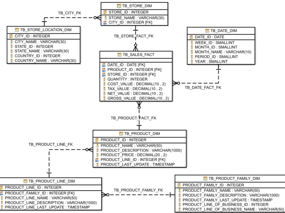
Physical data model design . . . 35
Implementation of the physical data model . . . . 36
Materialized query tables . . . 41
Replicated dimension tables . . . 44
Best practices summary . . . 47
Conclusion . . . 51
Important references. . . 53
Contributors . . . 55
Notices
. . . 57
Trademarks . . . 59 Contacting IBM . . . 59Index . . . 61
Executive Summary
This paper provides best practice recommendations that you can apply when designing a physical data model to support the competing workloads that exist in a typical 24×7 data warehouse environment.
It also provides a sample scenario with completed logical and physical data models. You can download a script file that contains the DDL statements to create the physical database model for the sample scenario.
This paper targets experienced users who are involved in the design and
development of the physical data model of a data warehouse in DB2 Database for Linux, UNIX, and Windows or IBM®InfoSphere®Warehouse Version 9.7
environments. For details about physical data warehouse design in Version 10.1 data warehouse environments, see “DB2 Version 10.1 features for data warehouse designs” on page 31.
For information about database servers in OLTP environments, see “Best practices: Physical Database Design for Online Transaction Processing (OLTP) environments” at the following URL:http://www.ibm.com/developerworks/data/bestpractices/
databasedesign/.
About this paper
This paper provides guidance to experienced database administrators and solution architects on physical data warehouse design for DB2 Database for Linux, UNIX, and Windows or IBM InfoSphere Warehouse environments and how to design a data warehouse for a partitioned database environment.
“Planning for data warehouse design” on page 5 looks at the basic concepts of data warehouse design and how to approach the design process in a partitioned data warehouse environment. This chapter compares star schema and snow flake schema designs along with their advantages and disadvantages.
“Designing a physical data model” on page 11 examines the physical data model design process and how to create tables and relationships.
“Implementing a physical data model” on page 15 describes the best approach to implement a physical model that considers both query performance and ease of database maintenance. It also describes how to incorporate DB2 capabilities such as database partitioning and using row level compression included with the IBM DB2 Storage Optimization Feature.
“Designing an aggregation layer” on page 27 explains how to aggregate data and improve query performance by using DB2 database objects such as materialized query tables.
The examples illustrated throughout this paper are based on a sample data warehouse environment. For details about this sample data warehouse
environment, including the physical data model, see “Data warehouse design for a sample scenario” on page 35.
Introduction to data warehouse design
A good data warehouse design is the key to maximizing and speeding the return on investment from your data warehouse implementation. A good data warehouse design leads to a data warehouse that is scalable, balanced, and flexible enough to meet existing and future needs. Following the best practice recommendations in this paper, you set your data warehouse up for long-term success through efficient query performance, easier maintenance, and robust recovery options.
Designing a data warehouse is divided into two stages: designing the logical data model and designing the physical data model.
The first stage in data warehouse design is creating the logical data model that defines various logical entities and their relationships between each entity.
The second stage in data warehouse design is creating the physical data model. A good physical data model has the following properties:
v The model helps to speed up performance of various database activities. v The model balances data across multiple database partitions in a clustered
warehouse environment.
v The model provides for fast data recovery.
The database design should take advantage of DB2 capabilities like database partitioning, table partitioning, multidimensional clustering, and materialized query tables.
The recommendations in this paper follow some of the guidelines for the IBM Smart Analytics System product to help you develop a physical data warehouse design that is scalable, balanced, and flexible enough to meet existing and future needs. The IBM Smart Analytics System product incorporates the best practices for the implementation and configuration of hardware, firmware, and software for a data warehouse database. It also incorporates guidelines in building a stable and scalable data warehouse environment.
Planning for data warehouse design
Planning a good data warehouse design requires that you meet the objectives for query performance in addition to objectives for the complete lifecycle of data as it enters and exits the data warehouse over a period of time.
Knowing how the data warehouse database is used and maintained plays a key part in many of the design decisions you must make. Before starting the data warehouse design, answer the following questions:
v What is the expected query performance and what representative queries look like?
Understanding query performance is key because it affects many aspects of your data warehouse design such as database objects and their placement.
v What is the expectation for data availability?
Data availability affects the scheduling of maintenance operations. The schedule determines what DB2 capabilities and partitioning table options to choose. v What is the schedule of maintenance operations such as backup?
This schedule affects your data warehouse design. The strategy for these operations also affects the data warehouse design.
v How is the data loaded into and removed from your data warehouse? Understanding how to perform these operations in your data warehouse can help you to determine whether you need a staging layer. The way that you remove or archive the data also influences your table partitioning and MDC design.
v Does the system architecture and data warehouse design support the type of volumes expected?
The volume of data to be loaded affects indexing, table partitioning, and maintaining the aggregation layer.
The recommendations and samples in this paper provide answers to these
questions. This information can help you in planning your data warehouse design.
Designing database models for each layer
Consider having a separate database design model for each of the following layers: Staging layer
The staging layer is where you load, transform, and clean data before moving it to the data warehouse. Consider the following guidelines to design a physical data model for the staging layer:
v Create staging tables that hold large volumes of fact data and large dimension tables across multiple database partitions.
v Avoid using indexes on staging tables to minimize I/O operations during load. Although, if data has to be manipulated after it has been loaded, you might want to define indexes on staging tables depending on the extract, transform, and load (ETL) tools that you use.
v Place staging tables into dedicated table spaces. Omit these table spaces from maintenance operations such as backup to reduce the data volume to be processed.
v Place staging tables into a dedicated schema can also help you. A dedicated schema can also help you reduce data volume for maintenance operations.
v Avoid defining relationships with tables outside of the staging layer. Dependencies with transient data in the staging later might cause problems with restore operations in the production environment. Data warehouse layer
The data warehouse tables are the main component of the database design. They represent the most granular level of data in the data warehouse. Applications and query workloads access these tables directly or by using views, aliases, or both. The data warehouse tables are also the source of data for the aggregation layer. The data warehouse layer is also called the system of record (SOR) layer because it is the master data holder and guarantees data consistency across the entire organization.
Data mart layer
A data mart is a subset of the data warehouse for a specific part of your organization like a department or line of business. A data mart can be tailored to provide insight into individual customers, products, or operational behavior. It can provide a real-time view of the customer experience and reporting capabilities.
You can create a data mart by manipulating and extracting data from the data warehouse layer and placing it in separate tables. Also, you can use views based on the tables in the data warehouse layer.
Aggregation layer
Aggregating or summarizing data helps to enhance query performance. Queries that reference aggregated data have fewer rows to process and perform better. These aggregated or summary tables need to be refreshed to reflect new data that is loaded into the data warehouse.
Designing physical data models
The physical data model of the data warehouse contains the design of each table and the relationships between each table. The implementation of the physical data model results in an operational database. Because of the high data volumes in a typical data warehouse, decisions that you make when developing the physical design of your data warehouse might be difficult to reverse after the database goes into production.
Plan to build prototypes of the physical data model at regular intervals during the data warehouse design process. Test these prototypes with data volumes and workloads that reflect your future production environment.
The test environment must have a database that reflects the production database. If you have a partitioned database in your production environment, create the test database with the same number of partitions or similar. Consider the scale factors of the test system compared to the production system when designing the physical model.
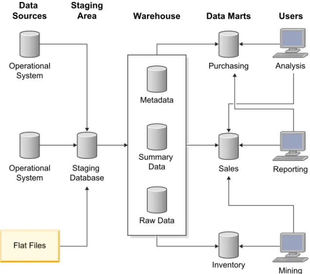
Figure 1 shows a sample architecture of a data warehouse with a staging area and data marts:
For details about the examples of the physical data model examples used in this paper, see“Data warehouse design for a sample scenario” on page 35.
Choosing between star schema and snowflake schema
A star schema and snowflake schema are based on dimensional modeling which is the recommended approach for data warehouse design. Use the schema design that best fits your needs for maximizing query performance.
A star schema might have more redundant data than a snowflake schema, especially for upper hierarchical level keys such as product type. A star schema might have relationships between various levels that are not exposed to the database engine by foreign keys. To choose better query execution plans, use additional information like column group statistics to provide the optimizer with knowledge of statistical correlation between column values of related level keys in dimensional hierarchies.
A snowflake schema has less data redundancy and clearer relationships between dimension levels than a star schema. However, query complexity increases as the join to the fact table has more dimension tables.
Place small dimensions such as DATE into one table and, as per the snowflake method, consider splitting large dimensions with over 1 million rows into multiple tables.
Data
Sources StagingArea Warehouse Data Marts Users
Operational System Metadata Summary Data Raw Data Purchasing Analysis Reporting Mining Sales Inventory Operational System Staging Database Flat Files
Figure 1. Sample architecture of a data warehouse
Regardless of what schema style you choose, avoid having degenerate dimensions in your schema. A degenerate dimension consists of a dimension in a single physical fact table. For example, avoid placing dimension data in fact tables. While row compression can substantially reduce the size of a table with redundant data, very large fact tables that are compressed can still present challenges with respect to the optimal use of memory and space for query performance.
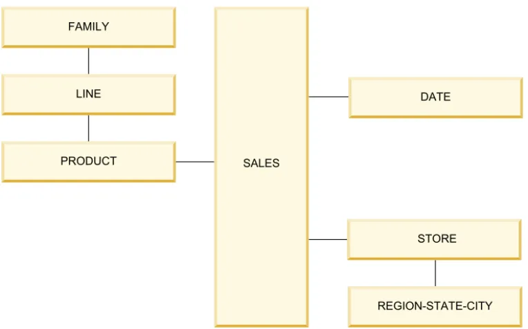
Figure 2 shows a data warehouse database model that uses both the star and snowflake schema:
A SALES fact table is surrounded by the PRODUCT, DATE, and STORE dimension tables.
The PRODUCT dimension is a snowflake dimension that has three levels and three tables because a large number of rows (row count) is expected.
The DATE dimension is a star dimension that has four levels (YEAR, QUARTER, MONTH, DAY) in a single physical table because a low row count is expected. The STORE dimension is partly denormalized. A table contains the STORE level and a second table that contains the REGION, STAGE, and CITY levels.
REGION-STATE-CITY STORE DATE FAMILY LINE PRODUCT SALES
Figure 3 shows the hierarchy of the dimension levels for Figure 2 on page 8:
Best practices
Use the following best practices when planning your data warehouse design: v Build prototypes of the physical data model at regular intervals during the
data warehouse design process. For more details, see “Designing physical data models” on page 6
v If a single dimension is too large, consider a star schema design for the fact table and a snowflake design such as hierarchy of tables for dimension tables. v Have a separate database design model for each layer. For more details, see
Database design layers.
All Products Family Line Product Product All Stores Region State City Store All Dates Year Quarter Month Date Store Day
Figure 3. Dimension levels hierarchy
Designing a physical data model
When designing a physical data model for a data warehouse focus on the definition of each table and the relationships between the tables.
When designing tables for the physical data model, consider the following guidelines:
v Define a primary key for each dimension table to guarantee uniqueness of the most granular level key and to facilitate referential constraints where necessary. v Avoid primary keys and unique indexes on fact tables especially when a large
number of dimension keys are involved. These database objects incur in a performance cost when ingesting large volumes of data.
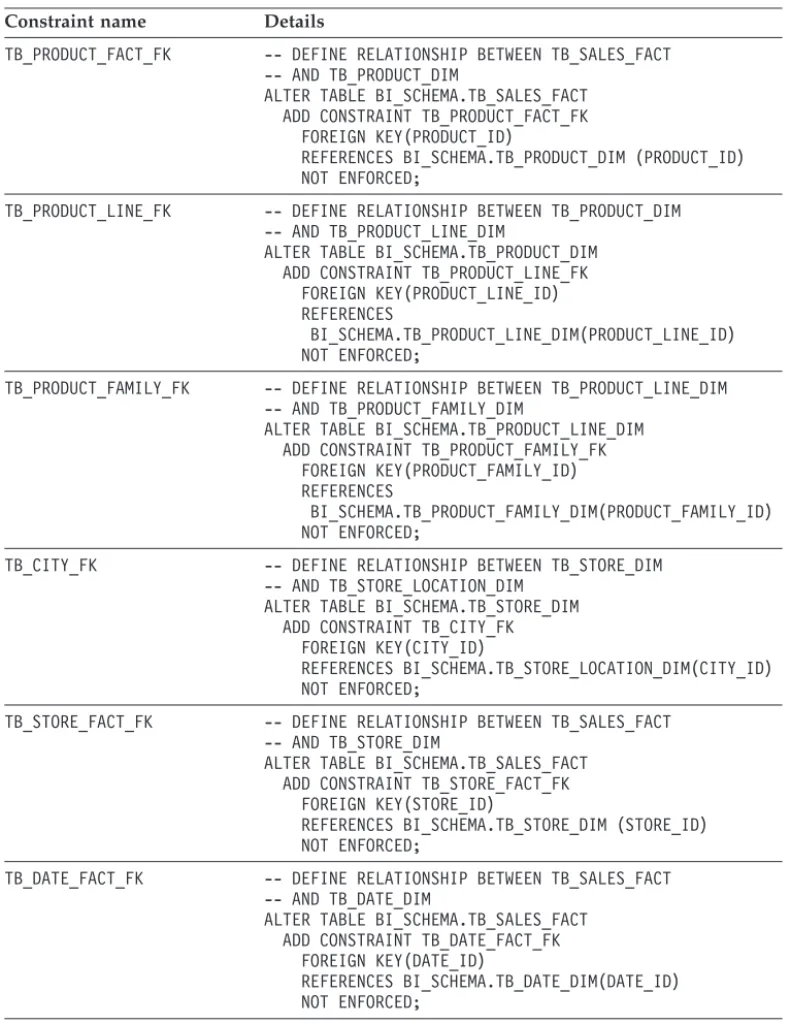
v Define referential constraints as informational between each pair of dimensions that are joined to help the optimizer in generating efficient access plans that improve query performance.
v Define columns with the NOT NULL clause. Identifying NULL values is a good indicator of data quality issues in the database and you should investigate before the data gets inserted into the database.
v Define foreign key columns as NOT NULL where possible.
v For DB2 Version 9.7 or earlier releases, define individual indexes on each foreign key to improve performance on star join queries.
v For DB2 Version 10.1, define composite indexes that have multiple foreign key columns to improve performance on star join queries. These indexes enable the optimizer to exploit the new zigzag join method. For more details, see “Ensuring that queries fit the required criteria for the zigzag join” at the following URL: http://publib.boulder.ibm.com/infocenter/db2luw/v10r1/topic/
com.ibm.db2.luw.admin.perf.doc/doc/t0058611.html.
v Define dimension level keys with the NOT NULL clause and based on a single integer column where appropriate. This way of defining level keys provides for efficient joins and groupings. For snowflake dimensions, the level key is
frequently a primary key which is commonly a single integer column.
v Implement standard data types across your data warehouse design to provide the optimizer with more options when compiling a query plan. For example, joining a CHAR(10) column that contains numbers to an INTEGER column requires cast functions. This join degrades performance because the optimizer might not choose appropriate indexes or join methods. For example, in DB2 Version 9.7 or earlier releases, the optimizer cannot choose a hash join or might not exploit an appropriate index.
For more details, see “Best Practices: Query optimization in a data warehouse” at the following URL:http://www.ibm.com/developerworks/data/bestpractices/ smartanalytics/queryoptimization/index.html.
Defining and choosing level keys
A level key is one column or a combination of columns in a table that uniquely identifies a hierarchy level within a dimension table. An example of a hierarchy of levels is DAY, WEEK, MONTH, YEAR in a date dimension. Another example is a column for the STORE dimension table that holds data for a retail store. A more complex example of level keys is the combination of the CITY, STATE, and COUNTRY columns in the same STORE table.
Level keys are used extensively in a data warehouse to join dimension tables to fact tables and to support aggregated tables and OLAP applications. The
performance of data warehouse queries can be optimized by having a good level key design.
A level key can be of one of the following types:
v A natural key identifies the record within the data source from which it originates. For example, if the CITY_NAME column has unique values in the dimension table, you can use it as a natural key to indicate the level in the CITY dimension.
v A surrogate key serves an identification purpose and helps reduce the size of a lower dimension table or a fact table. In most cases, a surrogate key is a single integer column. You can also use the BIGINT or DECIMAL data types for larger surrogate keys. For example, STORE_ID is a generated unique integer value that identifies a store. Using an integer instead of a large character string to
represents a store name or a combination of columns like STORE_NAME, CITY_NAME, and STORE_ID occupies less storage space in the fact table. Using surrogate keys for all dimension level columns helps in the following areas: v Increased performance through reduced I/O.
v Reduced storage requirement for foreign keys in large fact tables.
v Support slowly changing dimensions (SCD). For example, the CITY_NAME can change but the CITY_ID remains.
When dimensions are denormalized there is a tendency to not use surrogate keys. This example shows the statement to create the STORE dimension table without surrogate keys on some levels:
The STORE dimension is functionally correct because level keys can be defined to uniquely identify each level. For example, to uniquely identify the CITY level, define a key as [COUNTRY_NAME, STATE_NAME, CITY_NAME]. Unfortunately, a key that is a combination of three character columns does not perform as well as a single integer column in a table join or GROUP BY clause.
Consider the approach of explicitly defining a single integer key for each level. For queries that use a GROUP BY CITY_ID, STATE_ID, COUNTRY_ID clause instead of a GROUP BY CITY_NAME, STATE_NAME, COUNTRY_NAME clause, this approach works well. The following example shows the statement to create the STORE dimension table that uses this approach:
CREATE TABLE STORE_DIMENSION ( STORE_ID INTEGER NOT NULL, STORE_NAME VARCHAR(30), CITY_NAME VARCHAR(30), STATE_NAME VARCHAR(30), COUNTRY_NAME VARCHAR(30));
Collect “column group statistics” with theRUNSTATScommand in order to capture the statistical correlation between the surrogate key columns in addition to the correlation between the CITY_NAME, STATE_NAME and COUNTRY_NAME columns.
Guidelines for the date dimension
If a DATE column is used as a range partition column, the recommendation to use an INTEGER column as surrogate keys does not apply. Instead of an INTEGER column, use the DATE data type as the primary key on the date dimension table and as corresponding foreign key in the fact table.
Having a DATE column as the primary key for the date dimension does not consume additional space because the DATE data type length is the same as the INTEGER data types (4 bytes).
Using a DATE data type as a primary key enables your range partitioning strategy for the fact table to be based on this primary key. You can roll in or rollout data based on known date ranges rather than generated surrogate key values. In addition, you can directly apply date predicates that limit the range of date values considered for a query to a fact table. Also, you can transfer these date predicates from the dimension table to the fact table by using a join predicate. This use of date predicates facilitates good range partition elimination for dates not relevant to the query. If you need only the date range predicate for a query, you might even be able to eliminate the use of a join with the DATE dimension table.
The importance of referential integrity
Referential integrity (RI) constraints are defined primarily to guarantee the
integrity of data relationships between the tables. However, the optimizer also uses information about constraints to process queries more efficiently. Keep RI
constraints in mind as an important factor when designing your physical data model.
The following options are available when defining RI constraints: Enforced referential integrity constraints
The integrity of the relationship specified is enforced by the database manager when rows are inserted, updated, or deleted. There is a
performance effect on insert, update, delete, and load operations when the database manager must enforce RI constraints.
Informational constraints
Informational constraints are constraint rules that the DB2 optimizer can use but that are not enforced by the database manager. Informational
CREATE TABLE STORE_DIMENSION ( STORE_ID INTEGER NOT NULL, STORE_NAME VARCHAR(30), CITY_ID INTEGER, CITY_NAME VARCHAR(30), STATE_ID INTEGER, STATE_NAME VARCHAR(30), COUNTRY_ID INTEGER, COUNTRY_NAME VARCHAR(30));
constraints permit queries to benefit from improved performance without incurring on the overhead of referential constraints during data
maintenance. However, if you define these constraints, you must enforce RI during the ETL process by populating data in the correct sequences.
Best practices
Use the following best practices when designing a physical data model:
v Define indexes on foreign keys to improve performance on start join queries. For Version 9.7, define an individual index on each foreign key. For Version 10.1, define composite indexes on multiple foreign key columns.
v Ensure that columns involved in a relationship between tables are of the same data type.
v Define columns for level keys with the NOT NULL clause to help the optimizer choose more efficient access plans. Better access plans lead to improved performance. For more information, see “Defining and choosing level keys” on page 11.
v Define date columns in dimension and fact tables that use the DATE data type to enable partition elimination and simplify your range partitioning strategy. For more information, see “Guidelines for the date dimension” on page 13.
v Use informational constraints. Ensure the integrity of the data by using the source application or by performing an ETL process. For more information, see “The importance of referential integrity” on page 13.
Implementing a physical data model
Implementing a physical data model transforms the physical data model into a physical database by generating the SQL data definition language (DDL) script to create all the objects in the database.
After you implement a physical data model in a production environment and populate it with data, the ability to change the implementation is limited because of the data volumes in a data warehouse production environment.
The main goal of physical data warehouse design is good query performance. This goal is achieved by facilitating collocated queries and evenly distributing data across all the database partitions.
A collocated query has all the data required to complete the query on the same database partition. An even distribution of data has the same number of rows for a partitioned table on each database partition. Improving one these aspects can come at the expense of the other aspect. You must strive for a balance between
collocated queries and even data distribution.
Consider the following areas of physical data warehouse design: v Database partition groups
v Table spaces v Tables v Indexes
v Range partition tables v MDC tables
v Materialized query tables (aggregated or replicated)
The importance of database partition groups
Each table resides in a table space and each table space belongs to a database partition group. Each database partition group consists of one or more database partitions to which table spaces are assigned. When a table is created and assigned to a table space it is also assigned to the database partition group in which the table space exists.
Collocated queries can only occur within the same database partition group because the partition map is created and maintained at database partition group level. Even if the partitions covered by two database partition groups are the same, the database partitions have different partition maps associated with them. For this reason, different partition groups are not considered for join collocation.
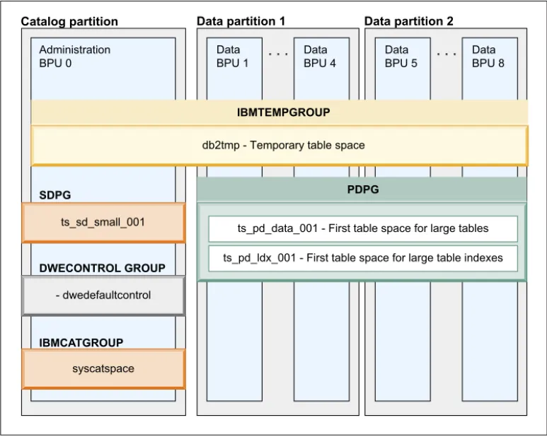
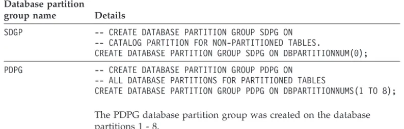
Implement a physical design model that follows the IBM Smart Analytics Systems best practices for data warehouse design. The IBM Smart Analytics Systems implementation has multiple database partition groups. Two of these database partition groups are called SDPG and PDPG. SDPG is created on the catalog partition for tables in one database partition. PDPG is created across each database partition and contains tables that are divided across all database partitions.
The following figure illustrates the database partition groups called SDPG and PDPG:
Consider the following guidelines when designing database partition groups: v Use schemas as a way of logically managing data. Avoid creating multiple
database partition groups for the same purpose.
v Group tables at the database partition group level to design a partitioned database that is more flexible in terms of future growth and expansion. Redistribution takes place at the database partition group level. To expand a partitioned database to accommodate additional servers and storage, you must redistribute the partitioned data across each new database partition.
Table space design effect on query performance
A table space physically groups one or more database objects for the purposes of common configuration and application of maintenance operations.
Discrete maintenance operations can help increase data availability and reduce resource usage by isolating these operations to related table spaces only. The following situations illustrate some of the benefits of discrete maintenance operations:
v You can use table space backups to restore hot tables and make them available to applications before the rest of the tables are available.
v You can find more opportunities to perform backups or reorganizations at a table space level because the required maintenance window is smaller.
Data BPU 1 Data BPU 4 Data BPU 5 Data BPU 8 Administration BPU 0
Catalog partition Data partition 1 Data partition 2
db2tmp - Temporary table space
ts_pd_data_001 - First table space for large tables ts_pd_ldx_001 - First table space for large table indexes
IBMTEMPGROUP PDPG IBMCATGROUP ts_sd_small_001 SDPG - dwedefaultcontrol syscatspace DWECONTROL GROUP
Good table space design has a significant effect in reducing processor, I/O, network, and memory resources required for query performance and maintenance operations.
Consider creating separate table spaces for the following database objects: v Staging tables
v Indexes
v Materialized query tables (MQTs) v Table data
v Data partitions in ranged partitioned tables
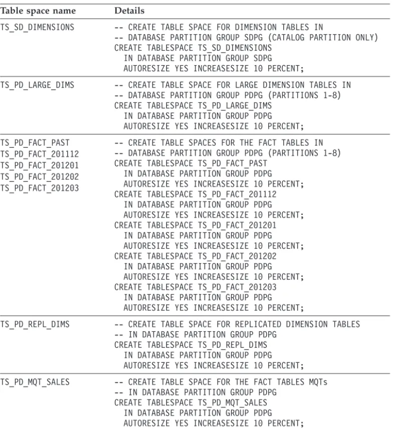
Creating too many table spaces in a database partition can have a negative effect on performance because a significant amount of system data is generated, especially in the case of range partitioned tables. Try to keep the maximum number of individual table partitions in hundreds, not in thousands. When creating table spaces, use the following guidelines:
v Specify a descriptive name for your table spaces.
v Include the database partition group name in the table space name.
v Enable the autoresize capability for table spaces that can grow in size. If a table space is nearly full, this capability automatically increases the size by the predefined amount or percentage that you specified.
v Explicitly specify a partition group to avoid having table spaces created in the default partition group.
Choosing buffer pool and table space page size
An important consideration in designing tables spaces and buffer pools is the page size. DB2 databases support page sizes of 4 KB, 8 KB, 16 KB, and 32 KB for table spaces and buffer pools.
In a data warehouse environment, large number of rows are fetched, particularly from the fact table, in order to answer queries. To optimize fetching of large number of rows, the IBM Smart Analytics System product uses 16 KB as the default page size. If you are using row compression, a large page size works better with large table spaces because they use large record identifiers (RIDs) and you can store more rows per page.
Using a large page size table space for the large tables must be weighted with other recommendations. For example, creating large tables as MDC tables is a best practice. However, a large page size can result in some wasted space. MDC tables that have dimensions on columns with a large number of distinct values or with skewed data that result in partially filled pages.
Another consideration is whether it makes sense to use table spaces with different page sizes to optimize access to individual tables. Each table space is associated with a buffer pool of the same page size. However, buffer pools can be associated with multiple table spaces. For optimum use of the total memory available to DB2 databases and use of memory across different table spaces, use one or at most two different buffer pools. Associating a buffer pool to multiple table spaces allows queries that access different table spaces at different times to share memory resources.
Reducing the number of different table space page sizes across the database helps you consolidate the associated buffer pools. Use one or, at most, two different page sizes for all table spaces. For example, create all table spaces with a 16 KB page size, a 32 KB page size, or both page sizes for databases that need one large table space and another smaller table space. Use only one buffer pool for all the table spaces of the same page size.
Table design for partitioned databases
Understanding the volumes of data intended for a table and how the table is joined with other tables in queries is important for a good table design in partitioned databases.
Because of the volumes of data involved in database partitioned tables, particularly fact tables, a significant outage is required to correct any data skew or collocation issues in post production. Outages require a considerable amount of organization. The columns used in the table partitioning key determine how data is distributed across the database partitions to which the table belongs. Choose the partitioning key from those columns in the table that have the highest cardinality and low data skew to achieve even distribution of data.
You can check the distribution of records in a partitioned table by issuing the following query:
The use of the sampling clause improves the performance of the query by using just a sample of data in the table. Use this clause only when you are familiar with the table data. The following text shows an example of the result set returned by the query:
For details about how to use routines to estimate data skews for existing and new partitioning key, see “Choosing partitioning keys in DB2 Database Partitioning Feature environments” at the following URL: http://www.ibm.com/developerworks/data/ library/techarticle/dm-1005partitioningkeys/.
In addition to even distribution of data, query performance is further improved by collocated queries that are supported by table design. If the query join is not collocated, the database manager must broadcast the records from one database partition to another over the network, which results in suboptimal performance.
SELECT DBPARTITIONNUM(DATE_ID) AS "PARTITION NUMBER", COUNT(1)*10 AS "TOTAL # RECORDS"
FROM BI_SCHEMA.TB_SALES_FACT TABLESAMPLE SYSTEM (10) GROUP BY DBPARTITIONNUM(DATE_ID)
ORDER BY DBPARTITIONNUM(DATE_ID);
PARTITION NUMBER TOTAL # RECORDS ---1 10,313,750 2 10,126,900 3 9,984,910 4 10,215,840
distribution of data across database partitions. Your table design must achieve the right balance between these competing requirements.
When designing a partitioned table, consider the following guidelines:
v Use partitioning keys that include only one column because fewer columns lead to a faster hashing function for assigning records to individual database
partitions.
v Achieve even data distribution. The data skew between database partitions should be less than 10%. Having one partition smaller-than-the-average by 10% is better than one partition larger-than-the-average by 10% to avoid having one database partition slower than the others. A slower partition results in slower overall query performance.
v Explicitly define partitioning keys. If a partitioning key is not specified, the database manager chooses the first column that is not a LOB or long field. This selection might not report optimal results.
When investigating collocation of data for queries consider the following guidelines:
v Collocation can occur only when the joined tables are defined in the same database partition group.
v The data type of the distribution key for each of the joined tables should be the same.
v For each column in the distribution key of the joined tables, an equijoin predicate is typically used in the query WHERE clause.
v The primary key and any unique index of the table must be a superset of the associated distribution key. That is, all columns that are part of the distribution key must be present in the primary key or unique index definition. The order of the columns does not matter.
The general recommendation for data warehouses is to partition the largest commonly joined dimension on its level key and partition the fact table on the corresponding foreign key. For most fact tables, this approach satisfies the requirement that the distribution key column has a very high cardinality, which helps ensure even distribution of data; the joins between a fact table and the largest commonly used dimension minimize data movement between database partitions.
For more information about how to address even distribution of data with the collocation of tables and improved performance of existing queries through
collocated table joins, see “Best Practices: Query optimization in a data warehouse” at http://www.ibm.com/developerworks/data/bestpractices/smartanalytics/queryoptimization/ index.html.
Partitioning dimension tables
After you decide to partition the fact table along with the largest commonly joined dimension table, you might need to move data for other dimension tables to collocate the data.
Most dimension tables in data warehouse environments are small and therefore do not benefit from being distributed across database partitions. Use the following recommendations when designing database partitioned tables:
v Partition the largest commonly joined dimension table on its level key collocated with the fact table because this table has the large number of unique values, which is good for avoiding data skew in the fact table.
v Place smaller dimensions into a table space that belongs a single database partition group.
v Replicate smaller dimension tables that belong to a single database partition group across all database partitions.
v Replicate only a subset of columns for larger dimension tables to avoid unnecessary storage usage when replicating data.
If a dimension table is not the largest in the schema, but still has a large number of rows (for example, over 10 million), you can replicate only a subset of the columns in the table. For more information about using replicated MQTs, see “Replicated MQTs” on page 28.
Range partitioned tables for data availability and performance
Table partitioning, also known as range partitioning, is a method that you can use to segment table data into separate data partitions. You can also assign data partitions to separate table spaces. Use range partitioning for any of the following reasons:
v Partitioning data into ranges to allow the optimizer to eliminate data partitions that are not needed to satisfy a query. This partition elimination helps to reduce I/O operations.
v Assign each data partition to an individual table space so that you can perform table space backups for a more strategic backup and data recovery design. v Roll in data partitions by using the ALTER TABLE statement with the ATTACH
parameter.
v Roll out data partitions by using the ALTER TABLE statement with the DETACH parameter.
v Minimize lock escalation because lock escalation in ranged partitioned tables happens at the partition level.
v Facilitate a multi-temperature data solution by moving data partitions from one temperature of storage tier to another as data ages.
For a data warehouse that contains 10 years of data and the roll-in/roll-out granularity is 1 month, creating 120 partitions is an ideal way of managing the data lifecycle. If the roll-in/roll-out granularity is by day, partitioning by day requires over 3600 partitions, which can cause performance and maintenance issues. An excessive number of data partitions increases the number of system catalog entries and can complicate the process of collecting statistics. Having too many range partitions can make individual range partitions too small for multidimensional clustering.
When using calendar month ranges in range partitioning, take advantage of the EXCLUSIVE parameter of the CREATE TABLE statement to simplify a lookup for month end date. The following example shows the use of the EXCLUSIVE parameter:
PARTITION PART_2011_DEC STARTING ('2011-12-01') ENDING('2012-01-01') EXCLUSIVE IN TBSP_2010_4Q;
Indexes on range partitioned tables
Indexes on range partitioned tables can be either global or local. Starting with DB2 Version 9.7 Fix Pack 1 software, indexes are created as local indexes by default unless they are explicitly created as global indexes or as unique indexes that do not include the range partitioning key.
A global index orders data across all data partitions in the table. A partitioned or local index orders data for the data partition to which it relates. A query might need to initiate a sort operation to merge data from multiple database partitions. If data is retrieved from only one partition or the partitioned indexes are accessed in order, including the range partitioning key as the leading column, a sort operation is not required.
Use global indexes for any of the following reasons:
v To enforce uniqueness on a column or set of columns that does not include the range partitioning key.
v To order the data across all partitions. You can also take advantage of global indexes to avoid a sort operation for an ORDER BY or a GROUP BY order requirement on the (leading) columns.
Use local indexes for any of the following reasons:
v Take advantage of the ability to precreate local indexes on data partitions before they are attached to the range partitioned table. Precreating local indexes minimizes any interruption when you use the ATTACH PARTITION or DETACH PARTITION parameter.
v Reduce I/O during ETL workloads as local indexes are typically more compact. If the inner join of a nested loop join or the range predicate in a query require probing multiple database partitions, multiple local indexes might be probed instead of a single global index. Incorporate these scenarios into your test cases.
Candidates for multidimensional clustering
Multidimensional clustering (MDC) tables can help improve the performance of many queries, reduce locking, and simplify table maintenance operations. In particular, MDC tables reduce the need to do a REORG to maintain data clustering.
Data in an MDC table is ordered and stored in a different way than regular tables. A table is defined as an MDC table through the CREATE TABLE statement. You must decide whether to create a regular or an MDC table during physical data warehouse design because you cannot change an MDC table definition after you create the table. Create MDC tables in a test environment before implementing them in a production environment.
An MDC table physically groups data pages based on the values for one or more specified dimension columns. Effective use of MDC can significantly improve query performance because queries access only those pages that have records with the correct dimension values.
The database manager creates a cell to reference each unique combination of values in dimension columns. An inefficient design causes an excessive number of cells to be created, which in turn increases the space used and negatively affects query performance. Follow these guidelines to choose dimension columns:
v Choose columns that are frequently used in queries as filtering predicates. These columns are usually dimensional keys.
v Create MDC tables on the columns that have low cardinality in order to have enough data to fill out entire cell.
v Create MDC tables that have an average of five cells per unique combination of values in the clustering keys. The more dimensions you can include in the clustering key, the higher is the benefit of using MDC tables.
v Use generated columns to reduce the number of distinct values for MDC dimensions in tables that do not have column candidates with suitable low cardinality.
For example, the BI_SCHEMA.SALES fact table in the sample scenario has three dimensions called STORE_ID, PRODUCT_ID, and DATE_ID that are candidates for dimension columns. To choose the dimension columns for this table, follow these steps:
1. Ensure that the BI_SCHEMA.SALES table statistics are current. Issue the following SQL statement to update the statistics:
RUNSTATS ON TABLE BI_SCHEMA.TB_SALES_FACT FOR SAMPLED DETAILED INDEXES ALL;
2. Determine whether the STORE_ID and DATE_ID columns are suitable as dimension columns. Use the following query to calculate the potential density of the cells columns based on an average unique cell count per unique value combination greater than 5:
SELECT CASE
WHEN (NPAGES/EXTENTSIZE)/
(SELECT COUNT(1) AS NUM_DISTINCT_VALUES
FROM (SELECT 1 FROM BI_SCHEMA.TB_SALES_FACT GROUP BY STORE_ID, DATE_ID)) > 5
THEN
'THESE COLUMNS ARE GOOD CANDIDATES FOR DIMENSION COLUMNS' ELSE
'TRY OTHER COLUMNS FOR MDC' END FROM SYSCAT.TABLES A, SYSCAT.TABLESPACES B
WHERE TABNAME='TB_SALES_FACT' AND TABSCHEMA='BI_SCHEMA' AND A.TBSPACEID=B.TBSPACEID;
If the BI_SCHEMA.SALES table is in a partitioned database environment, use the following query:
SELECT CASE
WHEN (NPAGES/EXTENTSIZE)/
(SELECT COUNT(1) AS NUM_DISTINCT_VALUES FROM (SELECT 1 FROM BI_SCHEMA.TB_SALES_FACT
GROUP BY DBPARTITIONNUM(STORE_ID),STORE_ID, DATE_ID)) > 5
THEN
'THESE COLUMNS ARE GOOD CANDIDATES FOR DIMENSION COLUMNS' ELSE
'TRY OTHER COLUMNS FOR MDC' END FROM SYSCAT.TABLES A, SYSCAT.TABLESPACES B
WHERE TABNAME='TB_SALES_FACT' AND TABSCHEMA='BI_SCHEMA' AND A.TBSPACEID=B.TBSPACEID;
The BI_SCHEMA.SALES table is range partitioned on the DATE_ID column. The range partitions for 2012 include a month of dates. For queries that have predicates by date, a date column helps to reduce the row access rows to 1 day out of 30 days in the month.
3. Create the BI_SCHEMA.SALES as an MDC table organized by the STORE_ID and DATE_ID columns in a test environment. Load the table with a
representative set of data.
4. Verify that the chosen dimension columns are optimal. Issue the following SQL statements to verify whether the total number of free pages (FPAGES) is close to the number of pages that contain data (NPAGES):
RUNSTATS ON TABLE BI_SCHEMA.TB_SALES_FACT; SELECT CASE
WHEN FPAGES/NPAGES > 2
THEN 'THE MDC TABLE HAS MANY EMPTY PAGES'
ELSE 'THE MDC TABLE HAS GOOD DIMENSION COLUMNS' END FROM SYSCAT.TABLES A
WHERE TABNAME='TB_SALES_FACT' AND TABSCHEMA='BI_SCHEMA';
If the number of free pages is double the number of data pages or more, then the dimension columns that you chose are not optimal. Continue repeating previous steps to test additional columns as dimension columns.
If you cannot find suitable candidates, use generated columns as dimension columns to reduce the cardinality of existing columns. Using generated columns works well for equality predicates. For example, if you have a column called PRODUCT_ID with the following characteristics:
v The values for PRODUCT_ID ranges from 1 to 100,000.
v The number of distinct values for PRODUCT_ID is higher than 10,000. v PRODUCT_ID is frequently used in predicates likePRODUCT_ID =
<constant_value>.
You can use a generated column on PRODUCT_ID divided by 1000 as a dimension column so that values range from 1 to 100. For a predicate like PRODUCT_ID = <constant_value>, access is limited to a cell that contains only 1/1000 of the table data.
Including row compression in data warehouse designs
Row compression can help you increase the performance of all database operations by reducing I/O and storage requirements for the database and maintenance operations. These requirements can become additional goals that align with your data warehouse design goals.
When designing a data warehouse, you must decide whether to compress a table or an index when they are created. In a data warehouse environment, use row compression on tables or index compression when your data servers are not CPU bound.
Row compression can significantly improve I/O performance through a better buffer pool hit ratio as more compressed data can be accommodated in the buffer pool.
Row compression does use additional CPU resources, so use row compression only in data servers that are not CPU bound. Because most operations in a data
warehouse read large volumes of data, row compression is typically a good choice
to balance I/O and CPU usage. If you perform many update, insert, or delete operations on a compressed table, use the PCTFREE 10 clause in the table definition to avoid overflowing records and consequent reorganizations. To show the current and estimated compression ratios for tables and indexes: v For DB2 Version 9.7 or earlier releases, use the
ADMIN_GET_TAB_COMPRESS_INFO_V97 and
ADMIN_GET_INDEX_COMPRESS_INFO administrative functions to show the current and estimated compression ratios for tables and indexes. The following example shows the SELECT statement that you can you use to estimate row compression for all tables in the BI_SCHEMA schema:
v For DB2 Version 10.1 and later releases, use the ADMIN_GET_TAB_COMPRESS_INFO and
ADMIN_GET_INDEX_COMPRESS_INFO administrative functions. The following example shows the compression estimates for a particular table ‘TB_SALES_FACT’:
If the workload is CPU bound, selective vertical compression or selective horizontal compression helps you to get storage savings at the cost of some complexity.
Selective vertical compression
If 5% of the columns in a table are accessed 90% of time, you can compress the fact table but keep an uncompressed MQT divided across all database partitions that has these frequently-accessed columns. Maintaining redundant data requires both administration and ETL overhead.
If relatively few columns are queried 90% of the time, a compressed table along with a composite uncompressed index on these columns is easier to administer
Selective horizontal compression
If the 90% of the data accessed is the most recent data, consider creating range partitioned tables with compressed historical data and uncompressed recent data. SELECT * FROM TABLE(SYSPROC.ADMIN_GET_TAB_COMPRESS_INFO_V97('BI_SCHEMA','','ESTIMATE'));
Best practices
Use the following best practices when implementing a physical data model: v Define only one partition group that spans across all data partitions as
collocated queries can only occur within the same database partition. For more details, see “The importance of database partition groups” on page 15. v Use a large page size table space for the large tables to improve performance
of queries that return a large number of rows. The IBM Smart Analytics Systems have 16 KB as the default page size for buffer pools and table spaces. Use this page size as the starting point for your data warehouse design. For more details, see “Choosing buffer pool and table space page size” on page 17.
v Hash partition the largest commonly joined dimension on its level key and partition the fact table on the corresponding foreign key. All other dimension tables can be placed in a single database partition group and replicated across database partitions. For more details, see “Table design for partitioned
databases” on page 18.
v Replicate all or a subset of columns in a dimension table that is placed in a single database partition group to improve query performance. For more details, see “Partitioning dimension tables” on page 19.
v Avoid creating a large number of table partitions or pre-creating too many empty data partitions in a range partitioned table. Implement partition creation and allocation as part of the ETL job. For more details, see “Range partitioned tables for data availability and performance” on page 20. v Use local indexes to speed up roll-in and roll-out of data. Corresponding
indexes can be created on the partition to be attached. Also, using only local indexes reduces index maintenance when attaching or detaching partitions. For more details, see “Indexes on range partitioned tables” on page 21. v Use multidimensional clustering for fact tables. For more details, see
“Candidates for multidimensional clustering” on page 21.
v Use administrative functions to help you estimate compression ratios on your tables and indexes. For more details, see “Including row compression in data warehouse designs” on page 23
v Ensure that the CPU usage is 70% or less of before enabling compression. If reducing storage is critical even in a CPU-bound environment, compress data that is infrequently used. For example, compress historical fact tables.
For more details about best practices for row compression, see “DB2 best practices: Storage optimization with deep compression” at the following URL:
http://www.ibm.com/developerworks/data/bestpractices/deepcompression/.
Designing an aggregation layer
Aggregating or summarizing data helps enhance query performance. Use DB2 database objects that help you aggregate data such as materialized query tables (MQTs), views, or view MQTs.
MQTs, also known as summary tables, precompute the results of an expensive or frequently used query or set of queries. The result set is stored in a dedicated table which can be used later to answer that frequently used query or similar queries. The source tables that are referenced when populating or refreshing data in an MQT are called base tables.
Using materialized query tables
Using MQTs to aggregate data at different levels, you can support applications that analyze data without having to design multiple base tables or compromise the atomic granularity of data.
Suboptimal performance of analytical queries is often the trigger point to use MQTs, especially in service level agreement (SLA) driven environments. Typically, you can define MQTs after you populate the fact tables and develop a set of important analytical queries.
MQTs can greatly improve query performance at the cost of extra storage and additional maintenance. The optimizer automatically reroutes your queries to the MQTs.
You can redesign MQTs over time as queries and the analysis of data evolves. From a design perspective, understand how MQTs are created, populated, and maintained to be able to choose the right type of MQT. You can create MQTs that use any of the following modes:
Refresh deferred
Use this mode in a data warehouse environment to control when the data is refreshed. This mode propagates changes made to the base tables to the MQT manually when you issue the REFRESH TABLE statement. You can control the selection of the MQT based on age of data by setting the dft_refresh_age database configuration parameter or the CURRENT REFRESH AGE special register. If the REFRESH AGE time limit is exceeded, the optimizer does not reroute your dynamic queries to MQTs. Refresh deferred with staging table
Use this mode when you have multiple ingest streams to update the base tables. Using this mode can help avoid locking the base tables in this situation. This mode automatically propagates changes made to the base table to a staging table specified when you created the MQT. To refresh the MQT that uses the staging table, issue the REFRESH TABLE statement. Refresh immediate
Use this mode in data warehouse environments where smaller volumes of data are involved. This mode automatically propagates the changes made to the base table to the MQT. The MQT remains current at all times. The INSERT, UPDATE, and DELETE operations on the base table carry with the overhead of MQT maintenance.
The following guidelines can help you improve the performance and increase usability of MQTs:
v Give a descriptive name to your MQT that includes the names of the base table and aggregation levels. Such naming convention helps in analysis of access plans and verification that the optimizer reroutes your queries to the right MQT for certain queries. An example for an MQT name that aggregates sales data by store, date, and product line is MQT_SALES_STORE_DATE_ PRODUCT. v If you are planning to use REFRESH IMMEDIATE or REFRESH DEFERRED
with MQT staging tables, create only one MQT per base table. If you have more than one MQT for a base table, the performance of update operations in the base table can decrease dramatically.
v If the base table has compression enabled, enable compression on the MQT as well. A compressed MQT becomes more competitive for query reroute by the DB2 optimizer.
v Improve the performance of the MQT refresh by creating an index on the base table that includes the columns specified in the GROUP BY clause of the MQT definition.
v For database partitioned base tables, improve the performance of the MQT refresh by creating MQTs in the same database partition group as the base tables. If possible, hash partition the MQT by using the same partitioning keys as the base fact table.
v For range partitioned base tables, improve the performance of the MQT refresh by creating MQTs as range partitioned tables on the same ranges as the base tables. Also, creating range partitioned MQTs makes MQTs more attractive candidates to the optimizer. If a table partitioning key column is also one of the dimensions to aggregate data in the MQT, you should not create a range partitioned MQT. For example, if you have a fact table range partitioned by MONTH and the MQT has GROUP BY MONTH, the range partitioned MQT table has only one row per month.
v Provide flexibility in a recovery scenario by creating MQTs in separate table spaces. It can be easier to re-create and refresh MQTs rather than restore them. v Create an MQT on a view for queries that use that view even if the view
contains constructs like outer joins or complex queries that are unsupported with regular MQT matching. For more details, see “Using views and view MQTs to define data marts” on page 29.
Replicated MQTs
Using replicated MQTs is a great technique to improve the performance of complex queries by copying the contents of a small dimension table to each database partition of a database partition group. For joins between a large database
partitioned table and a small dimension table, the query execution is faster because the data for the dimension table is replicated to each database partition and data transfer from other database partitions is not required.
Dimension tables typically have a few update operations. Therefore, specifying the REFRESH IMMEDIATE option to create replicated MQTs for small dimension tables makes the MQT maintenance free.
If your environment has many data partitions and the number of the replicated MQTs is significant, consider replicating only the subset of the columns that are referenced in your queries.
Because replicated MQTs are stand-alone objects, you must manually create
indexes similar to the indexes on the base tables. You should define unique indexes on the base tables as regular indexes on the replicated MQTs.
Using layered MQT refresh to improve maintenance
Using a layered MQT refresh approach to build MQTs takes advantage of existing MQTs. This approach is very useful for cubing applications where it is quite common to have aggregation on various dimension levels to support drill-downs and roll-ups, dozens of MQTs on various hierarchy levels, and a limited window to refresh MQTs.
The following steps shows an example on how to use a layered MQT refresh approach:
1. Create MQT1 defined on DATE_ID, STORE_ID, and PRODUCT_ID.
2. Create MQT2 defined on YEAR_ID, STORE_ID, PRODUCT_ID
3. Refresh MQT1.
4. Populate MQT2 by using the LOAD FROM CURSOR command on the base fact table. The optimizer reroutes the command to MQT1. The cursor is based on the MQT2 definition.
5. Set integrity for MQT2 using the UNCHECKED clause.
This method to populate MQT2 is faster because it only aggregates data in MQT1 by YEAR_ID and does not access the base fact table at all.
However, the database manager does not know about the similarities between different MQTs. Therefore, the sequence to issue the MQTs refresh is quite important. Create the indexes and collect statistics after MQTs are refreshed. For more information, see “Materialized query tables” on page 41.
Using views and view MQTs to define data marts
Views are a convenient way of hiding some details of the physical data model. They can express a business view of the world and enforce security rules within an organization. A view might encapsulate expressions that use the underlying object names and computations that the business user or the business application metadata model understands.
You can use views to define individual data marts based on the specific
requirements of individual lines of business that are different from the enterprise warehouse.
The advantages of views are:
v They do not require additional space.
v Their maintenance requirements are minimal.
v They simplify application development by hiding the complexity of the physical data model.
Data marts can be represented by using views over the base tables when the views are relatively simple. Carefully consider whether a view can represent a fact table. If a “fact view” gets too complex and includes operations such as UNION, LEFT OUTER JOIN, or GROUP BY queries that join the fact view with other dimension
table, views might have poor query performance when joined to other complex views. This performance issue might become apparent only when the number of queries and the database grow.
Starting with DB2 V9.7 or later versions, consider using view MQTs. You can create MQTs by simply selecting from a view. If you have a fact view for your data mart and you create a view MQT on that fact view, queries that access the fact view can be rerouted to the view MQT which looks as a simple fact table in the internally rewritten query.
Best practices
Use the following best practices when designing an aggregation layer:
v Use MQTs to increase the performance of expensive or frequently used queries that aggregate data. For more information, see “Using materialized query tables” on page 27.
v Use replicated MQTs to improve the performance of queries that use joins between a large database partitioned table and a small dimension table and reduce the intra-partition network traffic. For more information, see
“Replicated MQTs” on page 28
v Use views to define individual data marts when the view definition remains simple. For more information, see “Using views and view MQTs to define data marts” on page 29
DB2 Version 10.1 features for data warehouse designs
Use new features in DB2 Version 10.1 in your data warehouse to make your data lifecycle management easier, optimize storage utilization, and store and retrieve time-based data.
DB2 Version 10.1 introduces the following new features: v “Storage optimizations”
v “Multi-temperature data storage” v “Adaptive compression” on page 32
v “Time travel query by using temporal tables” on page 32
Storage optimizations
In DB2 Version 10.1, automatic storage table spaces have become the standard for DB2 storage because they provide the advantage of both ease of management and improved performance. For user-defined permanent table spaces, the SMS (system managed space) type is deprecated since Version 10.1. For more details about how to re-create SMS table spaces to automatic storage, see “SMS permanent table spaces have been deprecated” at the following URL:http://pic.dhe.ibm.com/infocenter/ db2luw/v10r1/topic/com.ibm.db2.luw.wn.doc/doc/i0058748.html.
Starting with Version 10.1 Fix Pack 1, the DMS (database managed space) type is deprecated. For more details about how to convert DMS table spaces to automatic storage, see “DMS permanent table spaces are deprecated” at the following URL: http://pic.dhe.ibm.com/infocenter/db2luw/v10r1/topic/com.ibm.db2.luw.wn.doc/doc/ i0060577.html.
You can now create and manage storage groups, which are groups of storage paths. A storage group contains storage paths with similar characteristics.
Automatic storage table spaces inherit media attribute values, device read rate, and data tag attributes from the storage group that the table spaces are using by default. Using storage groups has the following advantages:
v You can physically partition table spaces managed by automatic storage. You can dynamically reassign a table space to a different storage group by using the ALTER TABLESPACE statement with the USING STOGROUP option.
v You can create different classes of storage (multi-temperature storage classes) where frequently accessed (hot) data is stored in storage paths that reside on fast storage while infrequently accessed (cold) data is stored in storage paths that reside on slower or less expensive storage.
v You can specify tags for storage groups to assign tags to the data. Then, define rules in DB2 Work Load Manager (WLM) about how activities are treated based on these tags.
For more details, see “Storage management has been improved” in the DB2 V10.1 Information Center at the following URL:http://pic.dhe.ibm.com/infocenter/db2luw/ v10r1/topic/com.ibm.db2.luw.wn.doc/doc/c0058962.html.
Multi-temperature data storage
In a data warehouse environment, aligning active (hot) data with faster storage and inactive (cold) data with slower storage makes data lifecycle management
easier. Also, you can apply different maintenance operations to table spaces with different temperature. You can define as many temperatures of data as your environment requires depending on the different storage characteristics and the type of workload.
Another application in data warehouse environments is to use multi-temperature storage classes with range partitioned tables. After assigning table spaces to different storage groups to define multiple temperatures, assign each data partition to a table space with the appropriate temperature to prioritize the data access. You can create storage groups by using the CREATE STOGROUP statement to indicate the corresponding storage paths and device characteristics as shown in the following example:
CREATE STOGROUP hot-sto-group-name ON hot-sto-path-1, ..,hot-sto-path-N
DEVICE READ RATE hot-read-rate OVERHEAD hot-device-overhead
CREATE STOGROUP cold-sto-group-name ON cold-sto-path-1, ..,cold-sto-path-N
DEVICE READ RATE cold-read-rate OVERHEAD cold-device-overhead
After creating the storage groups, use the ALTER TABLESPACE statement to move automatic storage tables spaces from one storage group to another. Assign tables spaces that contain hot data to the hot storage groups and the table spaces that contain cold data to the cold storage group. Having the data accessed by most queries in the hot table spaces improves query performance substantially. For more details, see “DB2 V10.1 Multi-temperature data management recommendations” at the following URL:
http://www.ibm.com/developerworks/data/library/long/dm-1205multitemp/index.html.
Adaptive compression
In DB2 Version 10.1, adaptive compression uses page-level compression dictionaries in addition to the table-level compression dictionary to compress tables. Adaptive compression adapts to changing data characteristics and provides significantly better compression ratios in many cases because the page-level compression dictionary takes into account all of the data that exists within the page. In data warehouse environments, better compression rates translates into substantial storage reductions.
Page-level compression dictionaries are automatically maintained. Therefore, you do not need to perform a table reorganization to compress data on that page. In addition to improved compression rates, this approach to compression can improve the availability of your data and the performance of maintenance operations that involve large volumes of data. For more details, see “DB2 best practices: Storage optimization with deep compression” at the following URL:http://www.ibm.com/ developerworks/data/bestpractices/deepcompression/.
Time travel query by using temporal tables
Use temporal tables to associate time-based state information with your data. Data in tables that do not use temporal support apply to the present, while data in temporal tables can be valid for a period defined by the database system, user applications, or both.
With temporal tables, a warehouse database can store and retrieve time-based data without additional application logic. For example, a database can store the history of a table so you can query deleted rows or the original values of updated rows.
at the following URL:http://www.ibm.com/developerworks/data/bestpractices/temporal/ index.html.
Best practices
Use the following best practices to take advantage of new DB2 Version 10.1 features: v Use automatic storage table spaces. If possible, convert existing SMS or DMS
table spaces to automatic storage.
v Use storage groups to physically partition automatic storage table spaces in conjunction with table partitioning in your physical warehouse design. v Use storage groups to create multi-temperature storage classes so that
frequently accessed data is stored on fast storage while infrequently accessed data is stored on slower or less expensive storage.
v Use adaptive compression to achieve better compression ratios.
v Use temporal tables and time travel query to store and retrieve time-based data.