DIGITAL IMAGE ANALYSIS OF BURNING DROPLETS IN THE PRESENCE OF BACKLIGHT DIFFRACTION AND SOOT

DIGITAL IMAGE ANALYSIS OF BURNING DROPLETS IN

THE PRESENCE OF BACKLIGHT DIFFRACTION AND SOOT

R

B

B

D. S

1_{Department of Physics, University of Washington, Seattle;}2_{Department of Mechanical and Aerospace}

Engineering, University of California, Davis

e-mail: [email protected], [email protected]

(Received September 26, 2018; revised November 26, 2018; accepted November 28, 2018)

ABSTRACT

Approaches for analyzing digital images of moving and burning fuel droplets, with the goal of accurately measuring droplet edge coordinates, are discussed. Strategies for locating droplet edges in the presence of obscuration from soot and also backlight diffraction at the droplet edge are described. An outlier detection method is employed to identify outliers in droplet edge coordinates, and the resulting data can have significantly smaller standard deviations in droplet diameters if outliers are rejected, especially for droplets that exhibit significant soot formation. The approaches described herein are applied to images from droplet combustion experiments performed on the International Space Station as well as to synthetic image sequences that were generated to enable the accuracy of the algorithms to be assessed.

Keywords: burning droplets, diffraction, image analysis, soot.

INTRODUCTION

This research is in support of the Flame

Extinguishment Experiment (FLEX) and Flame

Extinguishment Experiment-2 (FLEX-2) droplet

combustion experiments that have been performed on the International Space Station (ISS). The FLEX and FLEX-2 research efforts employed reduced-gravity environments to investigate fundamental aspects of droplet combustion including liquid diffusion effects, gas diffusion effects including Soret diffusion, forced convective flows, sooting and droplet burning rates. The present research is focused on development of methods for analysis of droplet images from the ISS experiments, with a goal of providing accurate measurements of droplet size as a function of time. While the present research is focused on the ISS experiments, the methods described herein are also applicable to droplet images obtained from

ground-based experiments, e.g., drop tower and parabolic

flight aircraft facilities.

During an ISS experiment, the ends of two opposed hollow needles were manipulated to closely approach each other, at which point fuel is pumped through a needle, forming a droplet between the needles. The needles are then simultaneously retracted, leaving the droplet behind. The droplet could be free floating or deposited onto a thin support fiber, which prevented droplet drift. Initial droplet diameters were controllable and within the range 2–6 mm. After deployment, a droplet was ignited using two hot wire igniters symmetrically located on either side

of the droplet. The igniters were retracted following droplet ignition. In this research we consider only free (unsupported) droplets.

Images from each experiment were recorded with three different video cameras operating at 30 frame/s. The first camera, which was a color camera, provided real time information on droplet deployment, ignition, and overall experiment behavior. The second camera was monochrome and provided

high-resolution (1024×1024) images of droplets.

This camera was zoomed in on the droplets with a telecentric lens system. A droplet was backlit with collimated light from a laser diode such that the droplet image was the droplet shadow. The third camera was an intensified array camera that was used to image light in the ultraviolet portion of the spectrum. The images from each experiment were downloaded from the International Space Station as 16-bit TIFF images. Details on the experimental apparatus are available

elsewhere (Dietrichet al., 2013).

Information on droplet behavior, e.g., size and

position, is obtained from the backlit droplet view camera. Images from this camera are analyzed

frame-by-frame. Such information is useful, e.g., for

There are generally hundreds of TIFF images from any particular experiment, necessitating the use of computer image analysis techniques for timely analyses. Analysis of the backlit droplet view images often reduces to one task - determining the coordinates

of the liquid-gas interface, i.e., the droplet edge, at

several (or as many as possible) positions along the droplet edge. There are issues, however, that can be of importance when the present images are analyzed.

1. Soot particles can obscure the droplet edge.

2. There are backlight diffraction effects at the droplet edge.

3. There are small-scale background light variations, possibly from speckling, which cause variations in backlight intensity along the droplet edge.

4. There are large-scale background intensity light variations such that the average backlight intensity changes from one area of an image to another.

5. Free droplets can drift (change position) while they are burning.

Fig. 1 shows a typical image of a nonsooting and backlit droplet that is burning. This droplet is composed of n-heptane, which is a hydrocarbon species that is often present in practical liquid fuels. This image is a cropped from the original image, which had substantial negative space where no information was present that was useful for analysis. The droplet is the dark circle near the middle of the image. The flame is not visible because it is washed out by the much brighter backlight.

Fig. 1.Backlit image of a burning n-heptane droplet.

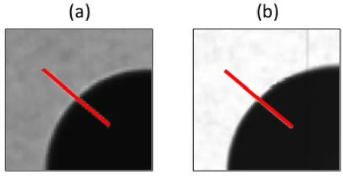
Fig. 2a shows the same droplet, but with a zoomed-in view showzoomed-ing the diffractive optical structure at the droplet edge. This structure, which is evident as the bright ring, is likely a result of partial coherence of the backlight. Variations in the average backlight intensity

as well as speckling over smaller length scales are also evident. Fig. 2b shows an image of a different droplet. In Fig. 2b, the background is bright enough that the camera pixels were mostly saturated such that the bright ring evident in Fig. 2a could not be evident.

Fig. 2.Zoomed-in non-sooting droplet images: (a) dim

background and (b) bright background.

The red lines in Figs. 2a and 2b are representative paths along which the pixel intensities are evaluated, as shown in Fig. 3. The bright region at the droplet edge in Fig. 2a corresponds to the peak in pixel intensity in Fig. 3 for the line marked as corresponding to the dim background. When the background light is bright enough to saturate the background (Fig. 3) the bright region at the droplet edge is not present (Fig. 2b).

Fig. 3.Radial line pixel intensity profiles for dim and

bright backgrounds.

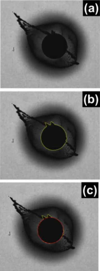
Fig. 4.Images showing: (a) a droplet with significant soot; (b) diffraction algorithm edge locations without outlier rejection (the yellow line); and (c) the droplet edge with outlier rejection (the red line overlapping the yellow line).

In this research we consider strategies for automated analysis of droplet images. Our specific goals are to implement a previously suggested algorithm to account for backlight diffraction effects and for local variations in background light levels, to evaluate a new edge detection method based on measurements of pixel intensity variations (noise) in droplet images, and to apply these algorithms to synthetic images as well as images from the ISS experiments.

Digital image analysis of burning droplets has been

previously studied (Choiet al., 1988; Dembia et al.,

2012; Aharonet al., 2013). These previous efforts did

not consider physical optics,i.e., diffraction and partial

coherence, when finding the edge of a backlit droplet. They also did not employ an algorithm based on measurements of image noise or use synthetic images

for evaluation of algorithm accuracy. These are topics we consider in the present research.

METHODS

The bases for our approach are the diffraction algorithm (DA) and the edge standard deviation (ESD) algorithm. The diffraction algorithm considers the effects of backlight diffraction at the droplet edge on images captured by a camera. As illustrated in Fig. 5, which exaggerates the thickness of the diffraction zone, we are interested in determining the edge coordinates of the geometric shadow of a droplet.

Diffraction Zone Diffraction Zone

Geometric Shadow Edge

Diffraction Zone Diffraction Zone

Geometric Shadow Edge

Droplet

Incident Light

Fig. 5. Schematic of the geometrical optics and

physical optics effects associated with formation of a shadow behind a droplet.

Diffraction effects, however, cause the edge of an

object in a backlit image to be diffuse (Fowler et al.,

2003; Senchenko et al., 2011). This behavior results

from constructive and destructive interference of light

after it passes by the droplet edge. Following (Yuet al.,

2014), we rescale the average intensities on either side of the diffraction zone such that the average intensity in the dark zone is zero and the average intensity in the bright zone is unity. If we term this rescaled

intensity In, then the droplet edge is located where

In = 0.5 if the incident light is purely incoherent and

at In = 0.25 if the incident light is purely coherent

(Fowler et al., 2003; Senchenko et al., 2011). For a

partially coherent backlight, which applies to these experiments, the droplet edge will be at a position

whereInis between 0.25 and 0.5.

We employed In = 0.31 as our partial coherence

edge intensity because this value was consistent with calibration images supplied by NASA. With our rescaled intensity, we calculate the droplets geometric shadow edge by interpolating around the pixels which

boundIn= 0.31. A best-fit circle is then fit to the points

case, we assume thatIn= 0.31 is applicable if at least

some of the background pixels are not saturated.

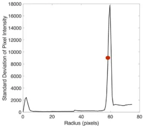
The ESD algorithm involves evaluating the pixel intensity profiles along circular-arc paths centered at the droplet center. The pixel intensities are nearly uniform within a droplet such that the standard deviation of intensity along a path is small. Outside the droplet edge, however, there are larger variations in intensity such that the standard deviation along a path will be significantly larger than for the droplet interior. At the droplet edge there is a transition zone where the standard deviation increases. The ESD algorithm is focused on locating this transition zone. A representative plot of the circular intensity standard deviation vs. radius (in pixels) for a droplet in the ISS experiments is shown in Fig. 6. The red dot corresponds to the droplet edge, which is assumed to be at the arithmetic average of the minimum and maximum standard deviation values.

Fig. 6.Representative ESD results.

Our decision tree runs through various techniques in order to process edge cases that arise in various situations. The algorithm is organized as follows.

1. The user of the software manually selects several points around the droplet periphery for the first image in a sequence to be analyzed.

2. A best-fit circle algorithm (K˚asa, 1976; Yuet al.,

2014) is used to provide an initial estimate of the droplet radius and center coordinates.

3. The diffraction algorithm is used to refine the droplet edge coordinates at N locations along the circle defined in step 2. Typically N = 100 or larger. The diffraction algorithm is applied along lines extending radially out from the droplet center

over a specified angular variation that corresponds to a portion of the droplet edge that is not highly obscured by soot.

4. A best-fit circle is generated using the refined edge points. This yields a new estimate for the droplet radius and center coordinates.

5. The Modified Thompson τ technique (ASME,

2013) at a 95 percent confidence level is applied to identify outliers in points marked as being at the droplet edge. This is accomplished by applying this test to the distance from each edge point to the droplet center.

6. The most extreme outlier is rejected.

7. Steps 4-6 are repeated until there are no more outliers.

8. The droplet center coordinates, the droplet radius, and the standard deviation in the droplet radius are saved.

9. The droplet center coordinates from step 8 are employed as input to the ESD algorithm to provide another measurement of the droplet radius.

10. The next image in the sequence is loaded for analysis.

11. The droplet edge coordinates from the previous image are employed as an initial estimate of the droplet edge coordinates of the image just loaded.

12. Steps 3-11 are repeated until all images have been analyzed.

The algorithm employed in the present analysis is implemented using Matlab (Mathworks, 2017).

As an assessment of the accuracy of our algorithms, we first apply them to synthetic droplet image sequences. These images were 1024 pixels by 1024 pixels, which are the same size as the backlit droplet images. These images were generated with the

Processing computer language (Reaset al., 2015).

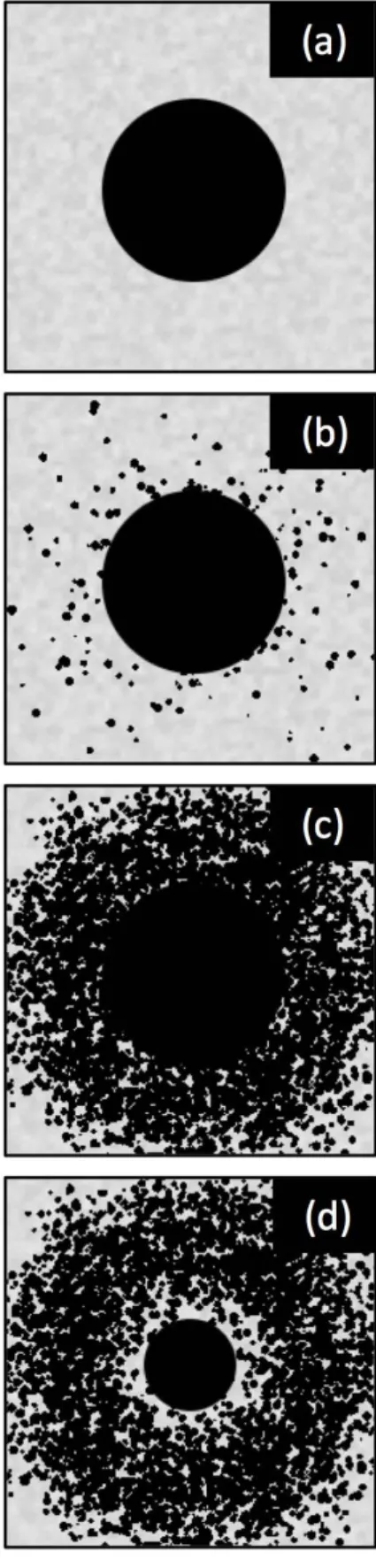
We consider three different synthetic image

sequences: (a) black droplet, gray speckled

background, and grayscale edge; (b) black droplet, gray speckled background, grayscale edge, and light sooting; and (c) black droplet, gray speckled background, grayscale edge, and heavy sooting. Each sequence had about 300 images.

fraction of pixel area covered by the geometric shadow of the droplet. This approach was adopted to account for the fact that in a backlit image, edge pixels will sometimes be partially obscured by the droplet such that the camera will record an average intensity for these pixels. A speckled background was simulated using Perlin noise (Perlin, 1985; Shiffman, 2012), and up to 5000 soot particles of random size and shape were included to simulate effects of edge obscuration by small and large soot particles. The soot particles were randomly clustered around a droplet. Fig. 7 shows a representative image from each sequence, and Fig. 8 shows the specified (exact) droplet diameter history that is applied when the image sequences are synthesized. The diameter history is specified to encompass a range that is representative of what is encountered in the ISS experiments.

We define the relative error E and the relative

standard uncertaintyUas shown in Eqs. 1 and 2 where

dm is the measured diameter,de is the exact diameter

specified for the synthetic image, andsdis the standard

deviation of the fitted droplet diameter:

E= (dm−de)/de, (1)

U =sd/de. (2)

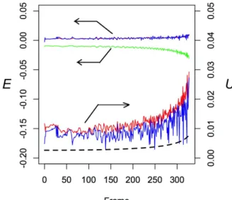
Fig. 9 shows frame-to-frame variations in E and

Ufor simulated image sequence (a),i.e., the sequence

that did not include soot. The dashed line is the

estimated minimum relative standard uncertaintyU_min,

which is defined in Eq. 3:

Umin=S/de. (3)

The variableSin Eq. 3 is the spatial resolution divided

by the square root of twelve, which is the standard deviation of a rectangular distribution. The spatial resolution is assumed to be one pixel for calculation

ofS. For the simulated images, and also for the ISS

images discussed below,S=0.0085 mm.

There are three relative error histories in Fig. 9: application of the DA without rejecting outliers (the red line); application of the DA with outliers rejected (blue line); and application of the ESD algorithm (green line). The DA results are very similar and it is difficult to distinguish them on the plot. The DA relative error magnitudes are typically less than 0.01. For comparison, the ESD relative error magnitudes are in the range 0.01–0.02.

Fig. 7. Simulated droplet images: (a) black droplet,

Fig. 8.Simulated droplet image diameter history.

The relative standard uncertainties in Fig. 9 are

of the order of 0.01–0.02, with the U values being

slightly larger when outliers are not rejected (the red line) relative to when outliers are rejected (the blue

line). Except for a few isolated points, U is greater

thanUmin in Fig. 9. When soot is not present, effects

of outliers onEandU are small.

Fig. 9.Relative error and relative standard uncertainty

histories for the simulated image sequence that did not include sooting: application of the DA without rejecting outliers (the red line), application of the DA with outliers rejected (blue line) and application of the ESD algorithm (green line).

Figs. 10 and 11 show results for E and U for

simulated image sequences (b) and (c), i.e., for light

and moderate sooting, respectively. The results in

Figs. 9, 10, and 11 indicate that the diffraction

algorithm works well unless the level of sooting is high enough to obscure most of the droplet edge (sequence (c)), and also that it is important to reject outliers for improved accuracy. It is noted that for sequence (c), the soot loading near the droplet surface was programmed to decrease with time, as is often observed in experiments, such that the droplet edge became progressively clearer as the droplet size decreased. This led to a better match with the known (exact) result over time. The ESD algorithm results are similar to the diffraction algorithm results, except that the ESD algorithm provides a better match to the exact droplet diameter values for high sooting levels. When significant sooting is present, an image will exhibit substantial variations in pixel intensity (noise) except for regions where the droplet blocks the backlight from

reaching the camera,i.e., the droplet shadow. The ESD

method assumes that image noise levels are small in the droplet shadow such that when noise levels are low then this is where the droplet resides.

The relative uncertainty increases with frame number in Fig. 9, regardless of whether outliers are rejected, because the uncertainty of a measurement is of the order of the uncertainty associated with the size of a pixel. From Eq. (2), as the droplet diameter decreases then the relative uncertainty increases if the standard deviation is unchanged. For Fig. 11, however, the relative uncertainty decreased with frame number because the soot loading near the droplet surface was programmed to decrease as the droplet size decreased, as shown in Fig. 7d.

Figs. 10 and 11 show that the presence of soot particles can have an appreciable influence on the performance of the DA algorithm. If outliers are not

rejected (the red lines), the E andU magnitudes are

appreciably larger than when outliers are rejected (the blue lines). The performance of the ESD algorithm is about the same for all three simulated image sequences.

RESULTS

Fig. 10. Relative error and relative standard uncertainty histories for the simulated image sequence with light sooting: application of the DA without rejecting outliers (the red line), application of the DA with outliers rejected (blue line) and application of the ESD algorithm (green line).

Fig. 11. Relative error and relative standard

uncertainty histories for the simulated image sequence with moderate sooting: application of the DA without rejecting outliers (the red line), application of the DA with outliers rejected (blue line) and application of the ESD algorithm (green line).

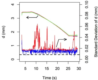
enhancement for the droplet edge to be visible. Fig. 12 shows results for droplet diameter as a function of time for an ISS propanol/glycerol mixture droplet that had small amounts of sooting. There are actually three plots in this Fig.. The red and blue lines are from application of the diffraction algorithm and the green line from application of the ESD algorithm. The red line is for when outliers are not rejected and the blue line is for when outliers are rejected. These three lines nearly overlap for the entire droplet history. This droplet extinguished at a time of about 25 s, which is why the droplet diameter does not change appreciably after this time. The data in Fig. 12 terminate at about 29 s because the droplet was drifting out of the field of view of the camera at this time.

Fig. 12.Droplet size variations for a negligible sooting

case.

Fig. 12 shows the standard deviation of the droplet diameter as a function of time both with and without rejection of outliers (the blue and red lines, respectively). For a negligible sooting case such as this, the influence of outliers is typically small.

Exceptions are during the ignition period, i.e., about

8–11 s in Fig. 12 and also when the droplet was leaving the field of view (about 29 s). During these times, the standard deviation including outliers is significantly larger than when outliers are rejected. Other large spikes in the standard deviation (including outliers) are from soot particles that were at the droplet edge from the perspective of the camera. Rejection of outliers reduces the standard deviation to levels that are

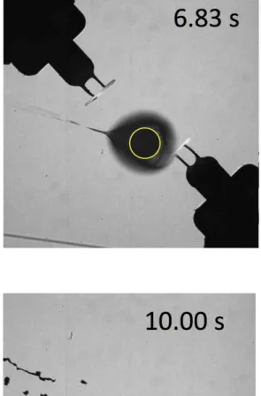
Fig. 13. Image sequence for a moderately-sooting case. The droplet edge is marked with a yellow circle.

An experiment with moderate sooting is defined here as when the edge of a droplet is obscured by soot, but where the diffraction and ESD algorithms can be

applied without altering the image, e.g., by altering

the pixel intensities to clarify the location of the droplet edge. An example image sequence is shown in Fig. 13. This image sequence is for a propanol/glycerol mixture droplet. Times are measured from the frame immediately following deployment needle retraction. The droplet edge is marked with a yellow circle in each figure.

Fig. 14 shows results on droplet diameter as a function of time from analysis of the moderately sooting droplet in Fig. 13. As before, the red and blue lines are from applying the diffraction algorithm and the green line the ESD algorithm. The blue line is where outliers are rejected and the red line is where outliers are not rejected. All three lines match well for most of the droplet history, though it is clear that rejecting outliers results in a smoother droplet size history with significantly reduced standard deviations after ignition, as shown with the red and blue lines in Fig. 14. The data terminate shortly after 14 s because the droplet left the field of view of the camera.

Fig. 14.Appreciably sooting droplet diameter analysis

results.

DISCUSSION

When possible, detection of the geometrical optics edge of a droplet should consider influences of diffraction. The diffraction algorithm discussed here worked well when soot obscuration of the edge of a droplet was negligible or nonexistent. It also worked well when the droplet edge was obscured, but where a portion of the edge was visible without applying image enhancement techniques. In this case, however, it is important to identify and reject outliers in order to reduce the uncertainty in the droplet diameter calculated with the circle curve fit. This will enable the standard deviations and uncertainties in calculations based on these measured values to be reduced. For example, rejecting outliers reduced the standard deviation in droplet diameter by as much as

about 0.06 mm and 0.3 mm in Figs. 12 and. 14,

respectively.

It is noted that the diffraction algorithm is not restricted to spherical shapes and could be used to determine the edge coordinates of non-spherical particles. For example, the edges of droplets undergoing shape oscillations could be detected.

The ESD algorithm also worked well for the cases discussed here. This algorithm is simple to use, but it requires a good estimate of the coordinates of the droplet center. The ESD algorithm does not currently provide information on the uncertainty of the fitted droplet diameter, though the algorithm could be extended to provide such estimates.

Future research could focus on identifying acceptable image enhancement techniques that could be used when the edge of a droplet is nearly completely obscured by soot. Because application of an image enhancement technique would likely change the optical structure of the diffraction zone, additional uncertainty would be introduced into the droplet edge coordinate measurements. Image enhancement approaches should be identified that minimize any added uncertainty.

In addition, based on Fig. 6, the rise in standard deviation is quite rapid at the droplet surface. As long as this is the case the uncertainty in the droplet radius is likely of the order of one or two pixels. The ESD approach could be further investigated, however, to better determine the value of the standard deviation that corresponds to the edge of a droplet.

ACKNOWLEDGEMENTS

The financial support of NASA via grant

NNX14AK01G is gratefully acknowledged. The Technical Monitor was Dr. Daniel L. Dietrich.

REFERENCES

Aharon I, Tam VK, Shaw, BD (2013). Combustion of submillimeter heptane/methanol and heptane/ethanol droplets in reduced gravity. J Combust 2013:154202. ASME (2013). Test Uncertainty. ASME Performance Test

Code 19.1. New York: American Society of Mechanical Engineers.

Choi MY, Dryer FL, Haggard JB, Brace MH (1988). Further observations of microgravity droplet combustion in the Nasa-Lewis drop tower facilities: A digital processing technique for droplet burning data. AIP Conf Proc 197:338-61.

Dembia CL, Liu YC, Avedisian, CT (2012). Automated data analysis for consecutive images from droplet combustion experiments. Image Anal Stereol 31:137– 48.

Dietrich DL, Ferkul PV, Byrg VM, Nayagam V, Hicks MC, Williams FA, Dryer FL, Shaw BD, Choi MY, Avedisian CT (2013). TP-2013-216046. Cleveland: NASA Glenn Research Center.

Fowler J, Litorja, M (2003). Geometric area measurements of circular apertures for radiometry at NIST. Metrologia 40:S9–S12.

K˚asa I (1976). A circle fitting procedure and its error analysis. IEEE T Instr Meas IM-25:8–14.

Mathworks (2017). Matlab version 9.3.0.713579 (R2017b). Natick: The Mathworks Inc.

Perlin K (1985). An image synthesizer. Proc 12th Ann Conf Comput Graph (SIGGRAPH’85) 287–96.

Reas C, Fry B (2015). Getting started with Processing, 2nd Ed. San Francisco: Maker Media, Inc.

Senchenko ES, Chugui YV (2011). Shadow inspection of 3D objects in partially coherent light. Meas Sci Rev 11:104–7.

Shiffman D (2012). The nature of code: Simulating natural systems with Processing. The Nature of Code.