Abstract— One of the most crucial steps in the design of
modern Embedded Systems (ES) is the partitioning the system’s functionalities between the hardware (HW) blocks and the software (SW) blocks. The process of hardware software partitioning (HSP) is driven by several non functional requirements factors. Several works studied the influence of the execution time and the hardware area (cost) factors while dealing with the HSP problem; other works included also the power consumption factor. This article gives a study the HSP problem while considering several factors (ES metrics) and presents two approaches to solve the problem. The first approach has the objective of optimizing simultaneously a number of metrics while respecting a constraint on the global hardware area (cost metric), this approach is implemented using 0-1 Knapsack Problem (KP) algorithm; experimental results show that the algorithm is very fast and gives more reliable solutions comparing to well-known algorithms such as the Genetic Algorithm (GA) and the Simulated Annealing (SA) algorithm. The second approach aims to optimize the hardware cost while respecting given constraints on the other metrics; the proposed approach is based on Balas method.
Index Terms—Embedded Systems, HW/SW Partitioning,
Multi-objective, 0-1 Knapsack Problem, Genetic Algorithm, Simulated Annealing, Balas Method.
I. INTRODUCTION
mbedded Systems consist of a combination of hardware components and one or more microprocessors executing software functionalities. The increasing complexity in designing embedded systems involves using high-level system approaches in order to achieve the system functionality and the performance goals. The compound design (Co-Design) is one of the most used approaches to fulfill the latter requirements. The goal is to enable robust system designs and to improve the hardware and the software interactions. The co-design is composed of four parts, co-specification to describe the system functionality at abstract level, co-synthesis to define the system architecture, co-simulation to simultaneously simulate the hardware and the software before prototyping, co-verification to verify mathematically that the system meets the requirements. The Hardware Software partitioning (HSP) process is the most important step in
co-synthesis part and in the whole co-design process. The HSP consists of splitting the system’s tasks into two parts, a hardware part and a software part, and choosing the best tasks to be included in each part based on some specific metrics and requirements.
Most of previous works dealt with the HSP problem with two metrics, the performance (execution time) and the cost (hardware area). In fact, the hardware leads to faster speed with more expensive cost while the software leads to cheaper cost with lower speed. The objective is to find the best possible balance between the performance and the cost. Two families of algorithms were proposed. On the one hand, the family of exact solutions such as Integer Linear Programming [1], Branch and Bound algorithm [2], and Dynamic Programming [3], are very successful for an HSP problem of a system with a small number of tasks. However, when the number of tasks increases, exact solutions tend to be slow and become inefficient. On the other hand, the family of heuristic algorithms gives an approximation to the exact solution, and it is very useful for an HSP problem of a system with large size. The most used heuristic algorithms are Simulated Annealing (SA) algorithm [4], Genetic Algorithm (GA) [5], Tabu Search algorithm [6] and Greedy Algorithm [7, 8].
Besides dealing with two metrics, other approaches were proposed to study the HSP problem with three metrics, execution time, hardware cost and power consumption metrics.
In this article, we propose two novel approaches with the objective of optimizing several metrics of the system. The metrics which are taken into account are the execution time, the hardware area, the power consumption, the development time (related to IP reuse), the quality (degree of maturity of the IP), the bandwidth and the memory usage. The first approach aims to optimize simultaneously the involved metrics with the respect of a given constraint on the global hardware area, while the second approach has the objective of optimizing the hardware area with the respect of the constraints on the involved metrics. For the first proposed approach, a weight is associated to each metric and is proportional to the important of this latter; the approach is based on the computation of the benefit of the implementation of the task in hardware; the approach is implemented using 0-1 Knapsack Problem algorithm; to validate its effectiveness,
HW/ SW Partitioning Algorithms for
Multi-objective Optimization in Embedded Systems
Adil Iguider, Oussama Elissati, Abdeslam En-Nouaary, and Mouhcine Chami
Institut National des Postes et Télécommunications, Lab. STRS,
Av. Allal El Fassi, Madinat Al Irfane, Rabat, Morocco.
Email: {iguider, elissati, abdeslam, chami}@inpt.ac.ma
we compare its results with the results obtained using Genetic Algorithm and Simulated Annealing algorithm. For the second approach, the total of each metric is calculated, and then, the Balas method is used to minimize the total hardware cost without exceeding the constraints on the other metrics.
The remainder of this article is organized as follows. Section II reviews the related works. In section III, we present the first proposed approach. In section IV, we give details of the implementations of this approach. The second proposed approach is presented in section V. Section VI shows the results of simulations. Lastly the conclusions and future works are summarized in section VII.
II. RELATED WORK
The co-design as defined in [9] is the design of cooperating hardware components and software components in a single design effort. Choosing a good balance between hardware implementation and software implementation is driving by several factors. Several works studied the influence of the execution time and the hardware cost while dealing with the HSP problem, either by exact solutions or by heuristic approaches.
The family of exact solutions includes algorithms, such as Integer Linear Programming (ILP), Branch and Bound algorithm (B&B), and Dynamic Programming (DP).ILP formulation consists of a set of variables, a set of linear inequalities, and a single linear function of the variables that serves as an objective function, in [1], the authors proposed to solve the HSP problem using ILP.B&B algorithm is based on binary tree, at each level, each variable can take the values 0 or 1, the objective is to find the path from the top to the bottom of the tree which has the optimal cost under the given constraints; an example of its application to the problem is presented in [2].DP is a method, in which large problems are broken down into smaller problems, and through solving the individual smaller problems, the solution to the larger problem is discovered, an example of using DP in the HSP problem is presented in [3].
The family of heuristic algorithms contains, inter alia, Simulated Annealing (SA) algorithm, Genetic Algorithm (GA), Tabu Search (TS) algorithm, Greedy Algorithm (GR), Hill Climbing (HC) Algorithm and Particle Swarm Optimization (PSO). With the analogy of solid annealing, the Simulated Annealing algorithm is based on a heating phase and a controlled cooling phase. An initial temperature is chosen and a first random solution is generated. Then the temperature is reduced and a neighbor solution is generated iteratively until the end of the cooling phase. In [4] the proposed algorithm is based on a combination of Simulated Annealing and Greedy Algorithm. In [10], the author proposed an enhanced algorithm for Simulated Annealing. Genetic algorithm is based on the survival of the fitness principle, which tries to retain more genetic information from generation to generation. The algorithm generates an initial population and defines a fitness function. The evolution of a generation is based on selection, crossover and mutation steps. The algorithm iterates over those steps and evaluates each
generation until certain condition is met and it returns the best individual of the latest generation as solution. In [5], the authors proposed and enhanced GA algorithm with an adaptive method for crossover and mutation steps. Other approaches were based on GA for solving the HSP problem, as in [11, 12]. Tabu Search algorithm picks an arbitrary point and evaluates an initial solution, then it computes the next set of solutions within neighborhood of current solution and picks the best solution from the set and iterates until the optima is reached. TS algorithm accepts non-improving solutions in order to escape from local optimum. In [6], the authors proposed two approaches, one is based on 0-1 Knapsack problem and the other is based on Tabu Search algorithm. Another implementation of the TS algorithm for the HSP problem was presented in [13]. Greedy Algorithm is based on making the locally optimal choice at each stage with the hope of finding the global optimum. In [7], the authors proposed three approaches based on Greedy Algorithm targeted for multi-processor system. In [8], the proposed algorithm is based on Greedy Algorithm and Simulated Annealing algorithm. Hill Climbing Algorithm consists of starting with a sub-optimal solution to a problem, and then repeatedly improves the solution until some condition is maximized; unlike the Greedy Algorithm, Hill Climbing Algorithm has the ability to avoid local minima; in [14], the authors proposed an algorithm based on HC for the HSP problem. Particle swarm optimization consists of a swarm of particles, where particle represent a potential solution (better condition). Particle will move through a multidimensional search space to find the best position in that space; an example of using PSO in hardware software partitioning is presented in [15].Other heuristic approaches were proposed to solve the HSP problem. In [16], the proposed approach is based on bat inspired algorithm. In [17] the authors proposed a methodology on Kernighan/Lin algorithm. In [18] the algorithm proposed is derived from the shortest path computing.
The previous cited articles deal with the HSP problem with two metrics. Other approaches were proposed to study the HSP problem with three metrics, execution time, hardware cost and power consumption metrics. In fact, minimizing the power consumption is particularly crucial for mobile devices and for the cost of the cooling system. In [19], the proposed algorithm is a combination of Genetic Algorithm and Branch and Bound Algorithm to simultaneously optimize the three metrics. In [20], the authors propose two heuristic algorithms to optimize the power consumption under execution time and area constraints for multiprocessor systems. In [21], the proposed algorithm is based on 0-1 Knapsack Problem and Tabu Search algorithm to simultaneously optimize the power and the execution time while respecting the hardware area constraint.
TABLEI
ALGORITHMS IN HW/SW PARTITIONING
Ref. Based algorithm Optimized metrics
Algo. Exact heuristic Exec time
HW area
Power
1 ILP * * *
2 B&B * * *
3 DP * * *
4 SA * * *
5 GA * * *
6 TS * * *
7 GR * * *
14 HC * * *
15 PSO * * *
16 BAT Inspired
* * *
17 Kernighan/ Lin
* * *
18 Shortest path * * *
19 GA + B&B * * * *
20 Tree Partitioning
* * * *
21 KP + TS * * * *
III. FIRST PROPOSED APPROACH
The goal of the first proposed approach is to optimize several metrics under the total hardware area constraint. In this study, we consider the following metrics: the execution time, the power consumption, the development time, the quality, bandwidth and the memory usage.
The system (ES) is composed of 𝑁blocks, denoted as
𝐵 = {𝐵1, 𝐵2, 𝐵3, … , 𝐵𝑛}. Each block 𝐵𝑖 can be implemented
either on hardware or on software.𝐻 denotes the set of blocks to be assigned to hardware and𝑆denotes the set of blocks to be assigned to software.
To each block𝐵𝑖considered implemented in hardware,
weassign a profit𝑃𝑖 and a weight 𝑎𝑖, the weight is supposed
tobe the area of the block in hardware, the profit is functionof the different other metrics: execution time, development time, power consumption, quality, bandwidth, memory usage. The profit of each block is calculated using the formula in the equation below:
𝑃𝑖= 𝜆1. (
𝑃𝑐𝑜𝑛𝑠𝑖𝑠 − 𝑃𝑐𝑜𝑛𝑠𝑖ℎ
𝑃𝑐𝑜𝑛𝑠𝑖𝑠 ) + 𝜆2. (
𝑇𝑒𝑥𝑒𝑐𝑖𝑠 − 𝑇𝑒𝑥𝑒𝑐𝑖ℎ 𝑇𝑒𝑥𝑒𝑐𝑖𝑠 ) + 𝜆3. (
𝑇𝑑𝑒𝑣𝑖𝑠 − 𝑇𝑑𝑒𝑣𝑖ℎ
𝑇𝑑𝑒𝑣𝑖𝑠 ) + 𝜆4. ( 𝑄𝑖ℎ− 𝑄𝑖𝑠
𝑄𝑖𝑠 ) + 𝜆5. ( 𝐵𝑑𝑖ℎ− 𝐵𝑑𝑖𝑠
𝐵𝑑𝑖𝑠 ) + 𝜆6. (
𝑀𝑒𝑚𝑖𝑠 − 𝑀𝑒𝑚𝑖ℎ
𝑀𝑒𝑚𝑖𝑠 ) (1)
For each block 𝐵𝑖:
- 𝑃𝑐𝑜𝑛𝑠𝑖ℎ and 𝑃𝑐𝑜𝑛𝑠𝑖𝑠 is respectively the power consumption
in hardware and in software.
- 𝑇𝑒𝑥𝑒𝑐𝑖ℎ and 𝑇𝑒𝑥𝑒𝑐𝑖𝑠 is respectively the time execution in
hardware and in software.
- 𝑇𝑑𝑒𝑣𝑖ℎ and 𝑇𝑑𝑒𝑣𝑖𝑠 is respectively the time of development
in hardware and in software, which may involve the IP reuse aspect.
- 𝑄𝑖ℎ and 𝑄𝑖𝑠 is respectively the quality of the block in
hardware and in software.
- 𝐵𝑑𝑖ℎ and 𝐵𝑑𝑖𝑠 is respectively the bandwidth in hardware
and in software.
- 𝑀𝑒𝑚𝑖ℎ and 𝑀𝑒𝑚𝑖𝑠 is respectively the shared memory
access in hardware and in software.
- The coefficients 𝜆1, 𝜆2, 𝜆3, 𝜆4, 𝜆5, and 𝜆6 are
positive integers used to give more or less importance to the associated criteria.
The objective is to find a partitioning (𝐻, 𝑆) for 𝐵such that:
𝐻 ∩ 𝑆 = ∅
and 𝐻 ∪ 𝑆 = 𝐵
With the maximization of the whole profit of the blocks that are implemented in hardware, while respecting the global hardware area constraint𝐴:
𝑚𝑎𝑥𝑖𝑚𝑖𝑧𝑒: ∑ 𝑃𝑖∗ 𝑥𝑖 𝑛
𝑖=1
𝑠𝑢𝑏𝑗𝑒𝑐𝑡 𝑡𝑜: ∑ 𝑎𝑖 𝑛
𝑖=1
∗ 𝑥𝑖 ≤ 𝐴
(2)
Where 𝑥𝑖 is the block’s implementation (HW=1, SW=0).
IV. IMPLEMENTATION
In this section we implement the proposed approach using three existent heuristic algorithms; the first algorithm is the 0-1 Knapsack Problem algorithm, the second algorithm is the Genetic Algorithm and the third algorithm is the Simulated Annealing algorithm.
A. 0-1 Knapsack Problem algorithm
The 0-1 Knapsack Problem is defined as follows:
1- Given number of items, where each item has a weight and a profit (integer numbers).
2- Given a knapsack with a maximum capacity (integer number).
3- The problem consists of choosing the items for which the total profit is maximized and the total weight doesn’t exceed the knapsack’s capacity.
The weight of each item (block) is the value of its hardware area, and its profit is calculated using (1).
In the first step, the profit of each block is calculated. If the profit is negative, the block is the moved to the software set (𝑆), elsewhere, the block is candidateto a hardware implementation.
𝑀 is the number of blocks candidates to hardware implementation. The pseudo-code ofthe 0-1 Knapsack algorithm is presented in Fig. 1.
1) Input: The array that contains the weights (hardware
area)of the blocks𝑊[1 … 𝑀]
2) Input: The array that contains the profits of the
blocks 𝑉[1 … 𝑀]
3) Input: The capacity 𝐴
4) Create a matrix 𝑇[0 … 𝑀; 0 … 𝐴]
5) 𝑇 is initialized with 0s
6) 𝑇 is then filled as follows:
For𝑖 = 0 𝑡𝑜 𝑀, for𝑗 = 0 𝑡𝑜 𝐴
a) If 𝑗 ≤ 𝑊[𝑖] ∶ 𝑇[𝑖, 𝑗] = 𝑇[𝑖 − 1, 𝑗]
b) else:
𝑇[𝑖, 𝑗] = max (𝑇[𝑖 − 1, 𝑗], 𝑉[𝑖] + 𝑇[𝑖 − 1, 𝑗 − 𝑊[𝑖])
7) Output: return 𝑇[𝑀, 𝐴]
Fig. 1. 0-1 Knapsack algorithm
The principle of the algorithm is to fill a matrix 𝑇 in recursive way based on the weights and the profits of the items.
The value of the last line and the last column of the constructed matrix (𝑇[𝑀, 𝐴]) gives the maximum possible profit. To find the selected items that make this maximum, an additional algorithm is necessary. This algorithm is described in Fig: 2.
1) 𝑖 = 𝑀; 𝑘 = 𝐴
2) 𝑤ℎ𝑖𝑙𝑒 𝑖 ≥ 1 𝑎𝑛𝑑 𝑘 ≥ 1
a) 𝑖𝑓 𝑉[𝑖, 𝑘] ≠ 𝑉[𝑖 − 1, 𝑘]:
i) mark the 𝑖𝑡ℎ block as selected
ii) 𝑖 = 𝑖 − 1
iii) 𝑘 = 𝑘 − 𝑊[𝑖]
b) else:
𝑖 = 𝑖 − 1
Fig. 2. 0-1 Knapsack algorithm: selected items
At the end, the selected blocks using KP algorithm are moved to the hardware set, while the unselected blocks are moved to the software set. The two constructed sets compose the solution to the initial problem defined in the previous section.
8) Example
The system is composed of four blocks; the profits and the weight of each block are as follows:
TABLEII KPPARAMETERS
Block Profit Weight
1 3 2
2 4 3
3 5 4
4 6 5
The capacity (hardware area constraint) is 𝐴 = 5, and:
𝑊 = [2, 3, 4, 5] 𝑉 = [ 3, 4, 5, 6]
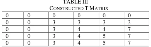
Using the algorithm of Fig. 1, the constructed matrix 𝑇 is as follows:
TABLEIII CONSTRUCTED TMATRIX
0 0 0 0 0 0
0 0 3 3 3 3
0 0 3 4 4 7
0 0 3 4 5 7
0 0 3 4 5 7
Using the algorithm of Fig. 2, the selected blocks are 1 and 2, therefore, the partitioning solution is:
𝑆 = {3, 4} 𝐻 = {1, 2}
B. Genetic Algorithm
The steps of the Genetic Algorithm are summarized in Fig. 3:
1) Initialize the parameters of the GA 2) generation := 1
3) Randomly generate an initial population of candidate solutions
4) Evaluate the population by computing the fitness of each individual
5) while (termination condition is not met) do: a) Create a new population
b) for each individual:
i) Select a parent based on its fitness
ii) Apply the crossover on the individual with its parents to produce an offspring
iii) Accept the crossover based on the fitness of the offspring
iv) Apply the mutation on the offspring
v) Accept the mutation based on the fitness of the offspring
vi) Add the offspring to the new population c) generation := generation + 1
d) Replace the old population by the new population e) Evaluate the new population
6) end loop;
7) return the best individual
An initial population (candidate solutions) is randomly generated. Then, each individual of the population is evaluated, its fitness (cost) is the sum of its hardware blocks profits. The termination test determines whether the process will stop or goes to the next generation. The process stops when the cost of the best solution (individual) for each generation no longer changes for a certain number of generations. When the process continues, a new population (generation) will replace the old one.
To generate a new population, three steps are applied on each individual. First step is the selection of the parent, in which the roulette wheel selection method is used; the individual with the highest fitness has more chance to be selected. Second, the process of crossover is applied to the individual with its parent to produce a new individual (offspring). If the offspring has less fitness or its hardware area is greater than the area constraint, then the crossover is rejected for this individual. The last step is the process of mutation, in this latter, the individual is randomly mutated (randomly selected blocks change the implementation between HW and SW) to generate a new offspring. Again, if the offspring has less fitness or its hardware area is greater than the area constraint, then the mutation is rejected for this individual. Then the algorithm iterates from the evaluation step. The process of elitism can also be applied in order to keep some few individuals with highest fitness from generation to generation.
C. Simulated Annealing algorithm
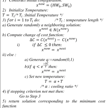
Simulated Annealing (SA) algorithm is based on the analogy between the solid annealing and the combinatorial optimization problem. The steps of the algorithm are summarized in Fig. 4:
1) Construct initial configuration: 𝑥𝑛𝑜𝑤 = (𝐻𝑊
0, 𝑆𝑊0) 2) Initialize Temperature:
𝑇 = 𝑇𝑖/* 𝑇𝑖 :Initial Temperature */
3) 𝑓𝑜𝑟 𝑖 = 1 𝑡𝑜 𝑇𝑙 do: /* 𝑇𝑙 : temperature length */ a) Generate randomly a neighboring solution:
𝑥𝑛𝑒𝑥𝑡 ∈ 𝑁(𝑥𝑛𝑜𝑤) b) Compute change of cost function:
∆𝐶 = 𝐶(𝑥𝑛𝑒𝑥𝑡) − 𝐶(𝑥𝑛𝑜𝑤)
i) 𝑖𝑓 ∆𝐶 ≤ 0 𝑡ℎ𝑒𝑛:
𝑥𝑛𝑜𝑤= 𝑥𝑛𝑒𝑥𝑡 ii) else :
a) Generate q:=random(0,1)
b)𝑖𝑓 𝑞 < 𝑒−∆𝐶𝑇 then: 𝑥𝑛𝑜𝑤= 𝑥𝑛𝑒𝑥𝑡 c) Set new temperature: 𝑇 = 𝛼 ∗ 𝑇
/* 𝛼 : cooling ratio */ 4) if stopping criterion not met then: Go to Step 3
5) return solution corresponding to the minimum cost function
Fig. 4. Simulated annealing algorithm
First, the algorithm starts by choosing an initial temperature, and randomly creates an initial solution (a HW set and a SW set). Second, in the generation step, a neighbor solution is created by randomly moving a block of the current solution from one set to the other set. Third, the process of acceptation is applied; the acceptance is function of the energy of the current solution, the energy of the neighbor solution and the actual temperature. The energy of each solution is related to the profit defined in (1). Fourth, the temperature is reduced. Lastly, the algorithm iterates from the generation step until certain condition is met (the energy doesn’t change).
V. SECOND PROPOSED APPROACH
The objective of the second proposed approach is to optimize the total hardware area under the constraints on the other metrics. The considered metrics: the execution time, the power consumption and the memory usage. The system is represented in the form of a directed acyclic graph (DAG) as shown in the example of Fig. 5.
Fig. 5. Example of DAG representation
Each block 𝐵𝑖 has the following values:
- 𝑃𝑐𝑜𝑛𝑠𝑖ℎ and 𝑃𝑐𝑜𝑛𝑠𝑖𝑠 : respectively the power consumption in
hardware and in software.
- 𝑇𝑒𝑥𝑒𝑐𝑖ℎ and 𝑇𝑒𝑥𝑒𝑐𝑖𝑠 : respectively the time execution in
hardware and in software.
- 𝐶𝑖ℎ and 𝐶𝑖𝑠 : respectively the cost of the hardware area
of the block in hardware and in software.
- 𝑀𝑒𝑚𝑖ℎ and 𝑀𝑒𝑚𝑖𝑠 : respectively the shared memory access
in hardware and in software.
- 𝑥𝑖represents the block’s implementation (in HW = 1,
in SW = 0)
As used in [22], the total cost and the total power consumption are given by (3) and (4):
𝐶 = ∑𝑛𝑖=1[(𝑥𝑖∗ 𝐶𝑖ℎ) + (1 − 𝑥𝑖) ∗ 𝐶𝑖𝑠] (3)
Each block 𝐵𝑖 is supposed to be executed upon the
reception of the corresponding data from its previous block
𝐵𝑖+1; therefore, as adopted in [22], the total execution time is
the sum of execution time of each block of the system:
𝑇 = ∑𝑛𝑖=1[(𝑥𝑖∗ 𝑇𝑒𝑥𝑒𝑐𝑖ℎ ) + (1 − 𝑥𝑖) ∗ 𝑇𝑒𝑥𝑒𝑐𝑖𝑠 ] (5)
We consider also that the total shared memory usage of the system is the sum of the shared memory usage of each block of the system:
𝑀 = ∑𝑛𝑖=1[(𝑥𝑖∗ 𝑀𝑒𝑚𝑖ℎ) + (1 − 𝑥𝑖) ∗ 𝑀𝑒𝑚𝑖𝑠 ] (6)
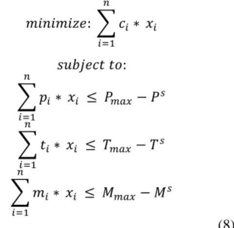
A. Problem formulation
We consider the problem that consists of minimizing the cost of the hardware area with the respect of the constraints on the other metrics:
𝑚𝑖𝑛𝑖𝑚𝑖𝑧𝑒: 𝐶
𝑠𝑢𝑏𝑗𝑒𝑐𝑡 𝑡𝑜:
𝑃 ≤ 𝑃𝑚𝑎𝑥 𝑇 ≤ 𝑇𝑚𝑎𝑥 𝑀 ≤ 𝑀𝑚𝑎𝑥
(7) Let:
𝐶𝑠= ∑ 𝐶𝑐𝑜𝑛𝑠𝑖𝑠 𝑛
𝑖=1
𝑃𝑠= ∑ 𝑃
𝑐𝑜𝑛𝑠𝑖𝑠 𝑛
𝑖=1
𝑇𝑠= ∑ 𝑇
𝑒𝑥𝑒𝑐𝑖𝑠 𝑛
𝑖=1
𝑀𝑠= ∑ 𝑀𝑖𝑠 𝑛
𝑖=1
And for each block 𝐵𝑖:
𝑐𝑖= 𝐶𝑖ℎ− 𝐶𝑖𝑠
𝑝𝑖= 𝑃𝑐𝑜𝑛𝑠𝑖ℎ − 𝑃𝑐𝑜𝑛𝑠𝑖𝑠
𝑡𝑖= 𝑇𝑒𝑥𝑒𝑐𝑖ℎ − 𝑇𝑒𝑥𝑒𝑐𝑖𝑠
𝑚𝑖= 𝑀𝑒𝑚𝑖ℎ − 𝑀𝑒𝑚𝑖𝑠
As 𝐶𝑠 is a constant value, the problem of (7) can be formulated as follows:
𝑚𝑖𝑛𝑖𝑚𝑖𝑧𝑒: ∑ 𝑐𝑖∗ 𝑛
𝑖=1 𝑥𝑖
𝑠𝑢𝑏𝑗𝑒𝑐𝑡 𝑡𝑜:
∑ 𝑝𝑖∗ 𝑛
𝑖=1
𝑥𝑖 ≤ 𝑃𝑚𝑎𝑥− 𝑃𝑠
∑ 𝑡𝑖∗ 𝑛
𝑖=1
𝑥𝑖 ≤ 𝑇𝑚𝑎𝑥− 𝑇𝑠
∑ 𝑚𝑖∗ 𝑛
𝑖=1
𝑥𝑖 ≤ 𝑀𝑚𝑎𝑥− 𝑀𝑠
(8)
The cost of the hardware area is bigger when the block 𝐵𝑖 is
implemented in HW; therefore the coefficients 𝑐𝑖 are all
positives. Consequently, the problem described in (8) can be resolved using the Balas’ technique.
B. Balas Method
The Balas’ algorithm is explained in [23]. Fig. 6 shows a simplified version of the steps of the algorithm.
Fig. 6. Simplified version Balas’ algorithm Set S= 0
Attempt to fathom S. Is the attempt successful?
If the best feasible completion of S has been found and is better than the incumbent, store it as the new incumbent. Augment S on the
right by 0 or 1 on any free variable.
Locate the rightmost element of S which is not fathomed. If none exists, terminate. Otherwise, replace the element by its
The method requires a LP in canonical form with 𝑐𝑖 ≥ 0 :
min 𝑧 = ∑ 𝑐𝑖∗ 𝑛
𝑖=1 𝑥𝑖
𝑥𝑖 ∈ {0, 1}
∑ 𝑎𝑖𝑗∗ 𝑛
𝑖=1
𝑥𝑖 ≤ 𝑏𝑗 1 ≤ 𝑗 ≤ 𝑚
(9)
The method is a tree method which progressively fixe to 0 or to 1 the variables 𝑥𝑖.
A vertex 𝑆𝑡 of the tree corresponds to a partial solution, for
which a subset 𝐹(𝑡) of variablesxi are fixed to 0 or 1.The
remaining variables form the set of free variables 𝐿(𝑡). In
𝐹(𝑡), we distinguish two subsets, the subset of variables fixed to 0 noted 𝐹0(𝑡), and the subset of variables fixed to 1 noted 𝐹1(𝑡). We choose a variable 𝑥𝑖 from 𝐿(𝑡) and we set it to 0 or
1 which gives two new nodes (children).
For each new created node 𝑆𝑡, the problem (9) becomes as
follows:
min 𝑧𝑡= ∑ 𝑐𝑖 𝑖∈𝐿(𝑡)
∗ 𝑥𝑖+ ∑ 𝑐𝑖 𝑖∈𝐹1(𝑡)
∑ 𝑎𝑖𝑗∗ 𝑥𝑖 ≤ 𝑏𝑗− ∑ 𝑎𝑖𝑗 = 𝑠𝑗1 ≤ 𝑗 ≤ 𝑚 𝑖∈𝐹1(𝑡)
𝑖∈𝐿(𝑡)
(10)
1) Node evaluation
After the creation of a new node 𝑆𝑡, it is evaluated. As the
objective is to minimize 𝑧𝑡, and as all the coefficients 𝑐𝑖 are
all positive, the evaluation of the node 𝑆𝑡 is as follows:
𝐸𝑣𝑎𝑙(𝑆𝑡) = ∑𝑖∈𝐹1(𝑡)𝑐𝑖 (11)
2) Node fathoming
After the creation of a new node𝑆𝑡, the following tests are
executed in order: a. Test 1:
𝑆𝑡 is abandoned if the evaluation of the node is
bigger than the provisional solution.
b. Test 2:
𝑆𝑡Is a terminal node if the evaluation of the node is
less than the provisional solution and all 𝑠𝑗 are
positives.
c. Test 3:
𝑆𝑡 is abandoned if the solution is not realizable.
This is the case for which some constraints are not satisfied:
∃ 𝑗 ∈ [1, 𝑚]: ∑ 𝑀𝑖𝑛(0, 𝑎𝑖𝑗) > 𝑠𝑗 𝑖∈𝐿(𝑡)
d. Test 4:
For any constraint (j), if the sum of negative 𝑎𝑖𝑗
but an 𝑎𝑝𝑗 is bigger than 𝑠𝑗 then 𝑥𝑝 is set to 1,and
if the sum of negative 𝑎𝑖𝑗 and a positive 𝑎𝑝𝑗 is
bigger than 𝑠𝑗 then 𝑥𝑝 is set to 0:
𝑖𝑓 ∃ 𝑗 ∈ [1, 𝑚] 𝑎𝑛𝑑 ∃ 𝑝 ∈ (𝑡) ∶
∑ 𝑀𝑖𝑛(0, 𝑎𝑖𝑗) + |𝑎𝑝𝑗| > 𝑠𝑗 𝑖∈𝐿(𝑡)
Then:
𝑥𝑝= 0 𝑖𝑓 𝑎𝑝𝑗> 0 𝑥𝑝= 1 𝑖𝑓 𝑎𝑝𝑗< 0
3) The choice of branching
The adopted method is called depth first; the deepest node is developed first. For the separation of branch on a variable𝑥𝑖,
the child node “𝑥𝑖= 1”is treated first. An index 𝑖 is associated
to each fixed variable in the form of “+𝑗” if 𝑥𝑖 is fixed to 1
and in the form of “−𝑗” if 𝑥𝑖 is fixed to 0.
Therefore, in the backtrack, the algorithm goes up until it reaches the top level above the variable from which the fathoming was done, if it is negative, it corresponds to a processed child, if it is positive, the algorithm takes the other branch, which corresponds to the complement of the value of that variable, and tries to fathom the new partial solution.
4) Decision of node separation
Let 𝑄(𝑡) = { 𝑗 |𝑠𝑗< 0 } the set of lines for which the
constraint is negative.
And 𝑅(𝑡) the set indexes of free variables 𝑥𝑖 having at least
one negative coefficient 𝑎𝑖𝑗 from 𝑄(𝑡):
𝑅(𝑡) = {𝑖 ∈ 𝐿(𝑡), ∃ 𝑗 ∈ 𝑄(𝑡), 𝑎𝑖𝑗 < 0}.
Let: 𝑃(𝑡) = ∑𝑗∈𝑄(𝑡)𝑠𝑗= ∑𝑚𝑗=1min (0, 𝑠𝑗).
The proximity of a solution if 𝑥𝑖 is set to 1 is:
𝑃(𝑡, 𝑖) = ∑ min (0, 𝑠𝑗− 𝑎𝑖𝑗) 𝑚
𝑗=1
(12)
The choice of the variable of separation 𝑖∗ is the variable
with the maximum proximity value:
𝑃(𝑡, 𝑖∗) = 𝑀𝑎𝑥{𝑃(𝑡, 𝑖)/𝑖 ∈ 𝑅(𝑡)}
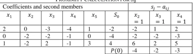
C. Example
In this example, we consider a system (ES) with 5 blocks
𝐵 = {𝐵1, 𝐵2, 𝐵3, 𝐵4, 𝐵5}.
The problem (8) to optimize is as follows:
𝑀𝑖𝑛: 3𝑥1+ 5𝑥2+ 4𝑥3+ 10𝑥4+ 𝑥5
2𝑥1− 3𝑥3− 4𝑥4+ 𝑥5 ≤ −2 (1)
−2𝑥2− 2𝑥3− 𝑥4≤ −4 (2)
𝑥1− 2𝑥2+ 2𝑥3− 𝑥4+ 3𝑥5≤ 4 (3)
𝑥𝑖 ∈ {0,1}, 1 ≤ 𝑖 ≤ 5
1) The root node 𝑆0
For the node 𝑆0:
𝐿(0) = {1, 2, 3, 4, 5} 𝑄(0) = {1, 2},
𝑅(0) = {2, 3, 4}
The evaluation of 𝑆0is 0. The proximity calculation is given
in table IV.
TABLEIV
PROXIMITY CALCULATION FOR 𝑆0
Coefficients and second members 𝑠𝑗− 𝑎𝑖𝑗
𝑥1 𝑥2 𝑥3 𝑥4 𝑥5 𝑆0 𝑥2
= 1 𝑥3
= 1 𝑥4
= 1
2 0 -3 -4 1 -2 -2 1 2
0 -2 -2 -1 0 -4 -2 -2 -3
1 -2 2 -1 3 4 6 2 5
𝑃(0) -4 -2 -3 The maximum proximity is obtained at 𝑥3, 𝑥3is therefore
the point of separation. We start by the branch 𝑥3= 1, the
branch 𝑥3= 0 will be processed later.
2) The node 𝑆1
For the node 𝑆1:
𝑥3= 1 𝐿(1) = {1,2,4,5}
𝐹1(1) = {3} 𝑄(1) = {2} 𝑅(1) = {2,4}
The evaluation of 𝑆1is 4. The completion of the other
variables (𝑥1= 𝑥2= 𝑥4= 𝑥5= 0) gives a non-realizable
solution as the constraints (2) is violated (−2 ≤ −4), therefore 𝑆1 is not a provisional solution.
The proximity calculation for 𝑆1is given in table V.
TABLEV
PROXIMITY CALCULATION FOR 𝑆1 Coefficients and second
members
𝑠𝑗− 𝑎𝑖𝑗
𝑥1 𝑥2 𝑥4 𝑥5 𝑆1 𝑥2
= 1 𝑥4
= 1
2 0 -4 1 1 1 5
0 -2 -1 0 -2 0 -1
1 -2 -1 3 2 4 3
𝑃(1) 0 -1
The maximum proximity is obtained at 𝑥2, 𝑥2 is therefore
the point of separation. We start by the branch 𝑥2= 1, the
branch 𝑥2= 0 will be processed later. The solution 𝑆1is then
marked with “+j”.
3) The node 𝑆2
For the node 𝑆2: 𝑥3= 1, 𝑥2= 1
𝐿(2) = {1, 4, 5} 𝐹1(2) = {2, 3}
The evaluation of 𝑆2is 9. The completion of the other
variables (𝑥1= 𝑥4= 𝑥5= 0) gives a realizable solution,
therefore 𝑆2 is a provisional solution and 𝑆2 is a terminal node.
4) The node 𝑆3
This node corresponds to a backtrack situation, we go back until the top of the branch, in this case we go back until 𝑆0 and
we process the branch 𝑥3= 0 and we mark 𝑆0 with “-j“. The
node 𝑆3 is abandoned as it leads to a non-realizable solution.
In fact, the test 3 fails, because for the constraint (2) we have:
∑𝑖∈𝐿(𝑡)𝑀𝑖𝑛(0, 𝑎𝑖𝑗) > 𝑠𝑗 :
−3 > −4
5) The node 𝑆4
We go down until a node marked with “+j“. In this case, we process the right hand of 𝑆1 and we mark 𝑆1 with “-j“.
For 𝑆4: 𝑥3= 1, 𝑥2= 0
𝐿(4) = {1,4,5} 𝐹1(4) = {3} 𝐹0(4) = {2}.
The node 𝑆4 is abandoned as it leads to a non realizable
solution. In fact, the test 3 fails, because for the constraint (2) we have:
∑𝑖∈𝐿(𝑡)𝑀𝑖𝑛(0, 𝑎𝑖𝑗) > 𝑠𝑗 :
−1 > −2
6) Termination
The algorithm terminates there is no node to process. The solution found in the node 𝑆2 is the optimal solution: 𝑥1= 𝑥4= 𝑥5= 0 and 𝑥2= 𝑥3= 1, the evaluation is 9. The
developed tree is shown in Fig. 7.
The solution of the HSP problem is then: - The blocks {𝐵2, 𝐵3} are in HW
- The blocks {𝐵1, 𝐵4, 𝐵5} are in SW.
VI. EXPERIMENTS
In this section we give the results of experiments for the first proposed approach.
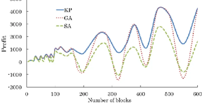
We implemented the three algorithms (0-1 Knapsack Problem algorithm, Genetic Algorithm, Simulated Annealing algorithm) in Java, and made a number of tests for different number of blocks. The metrics, the coefficients and the hardware area constraint are generated randomly. The metrics of each block are reel numbers and the software execution time of each block is always bigger than the hardware execution time. The coefficients are strictly positive integers. The hardware area constraint is and integer number smaller than the sum of the hardware area of all blocks.
Fig. 8 gives the comparison of the profit obtained using the three algorithm (KP, GA and SA). The results show that the profit obtained using KP algorithm and GA algorithm are almost identical and always bigger than the profit obtained using SA algorithm. GA and SA algorithms fail to converge in some cases, especially with small values of hardware area constraint.
Fig. 8. Comparison between the profits of algorithms
Fig. 9 gives the hardware area obtained for each algorithm. In case of non-convergence, the GA and SA algorithms don’t respect the hardware area constraint. This latter is always respected by KP algorithm.
Fig. 9. HW area of algorithms vs. HW area constraint
Fig. 10 gives a comparison between the algorithms in term of their execution time. The results show that KP and SA are very fast comparing to GA algorithm.
Fig. 10. Algorithms’ execution time comparison
VII. CONCLUSION
In this article, we proposed two novel approaches to solve the multi-objective Hardware Software Partitioning problem. The first approach aims to optimize several metrics under a constraint on the global hardware area. The second approach has the objective of minimizing the global hardware area while respecting the constraints on the other metrics. The principle of the first approach is based on the profit obtained when implementing each block in hardware. The profit is a weighted sum function of each metric’s benefit when the block is implemented in hardware over its implementation in software. The approach is implemented using 0-1 Knapsack Problem algorithm and compared to Genetic Algorithm and Simulated Annealing algorithm. Experimental results show that the KP algorithm is the best choice to implement the proposed approach; in fact, KP is very fast and gives best solutions comparing to GA and SA algorithms. The principle of the second approach is based on Balas method. As future works, we will implement the second proposed approach, and compare the two approaches with recent algorithms. We will also demonstrate their effectiveness on some practical examples.
REFERENCES
[1] R. Niemann and P. Marwedel, “Hardware/software partitioning using integer programming,” in Proceedings of the 1996 European conference on Design and Test, 1996, p. 473.
[2] W. Jigang and S. Thambipillai, “A branch-and-bound algorithm for hardware/software partitioning,” in Proceedings of the Fourth IEEE International Symposium on Signal Processing and Information Technology, 2004, pp. 526–529.
[3] P. V. Knudsen and J. Madsen, “Pace: A dynamic programming algorithm for hardware/software partitioning,” in Proceedings of the 4th International Workshop on Hardware/Software Co-Design, 1996, p. 85.
[4] Y. Jing, J. Kuang, J. Du, and B. Hu, “Application of improved simulated annealing optimization algorithms in hardware/software partitioning of the reconfigurable system-on-chip,” Communications in Computer and Information Science, vol. 405, 2014.
[5] C. W. Jinfu Feng, Junhua Hu and D. Qi, “Hardware/software partitioning algorithm based on genetic algorithm,” Journal of Computers, vol. 9, pp. 1309–1315, 2014.
[6] J. Wu, P. Wang, S.-K. Lam, and T. Srikanthan, “Efficient heuristic and tabu search for hardware/software partitioning,” The Journal of Super computing, vol. 66, pp. 118–134, 2013.
[8] L. Zhang, C. Xu, T. Zheng, and T. Li, “Hardware/software partitioning based on greedy algorithm and simulated annealing algorithm,” Journal of Computer Applications, vol. 33, no. 07, p. 1898, 2013.
[9]Chaumont, P. A practical introduction to hardware/software codesign. New York: Springer. 2013.
[10] Banerjee, S. &Dutt, N. Very fast simulated annealing for hw-sw partitioning. Technical Report, CECS-TR-04--17. 2004.
[11]Madhura, P. & Marek R. & Witold P. Genetic algorithms for hardware software partitioning and optimal resource allocation. Journal of Systems Architecture, l (53), 339 – 354. 2007
[12]Knerr, B. &Holzer, M. & Rupp, M. (2007).Novel genome coding of genetic algorithms for the system partitioning problem. International Symposium on Industrial Embedded Systems, SIES'07.134-141.
[13] Lin, G. & Zhu, W. & Ali, M. A tabu search-based memetic algorithm for hardware/software partitioning. Mathematical Problems in Engineering. 2014. [14]Sim, J. &Mitra, T. & Wong, W. Defining neighborhood relations for fast spatial-temporal partitioning of applications on reconfigurable architectures. International Conference on International Conference on, 121-128. 2008 [15]Farmahini-Farahani, A. & Kamal, M. & Fakhraie, S. & Safari, S. HW/SW partitioning using discrete particle swarm. Proceedings of the 17th ACM Great Lakes symposium on VLSI, 359-364. 2007
[16]Prakasam, S. & Venkatachalam, M. &Saroja, M. &Pradheep, N. &Gowthaman P. A novel bat inspired algorithm for hardware-software codesign partitioning. International Journal of Multidisciplinary Research and Development, l (3), 88-92. 2016
[17]Knerr, B. &Holzer, M. & Rupp, M. HW/SW partitioning using high level metrics. 2004
[18] Wu, J. &Srikanthan, T. & Zou, G. New model and algorithm for hardware/software partitioning. Journal of Computer Science and Technology, l(23), 644-651. 2008
[19] J. Resano, D. Mozos, E. Perez, H. Mecha, and J. Septien, “A hardware/ software partitioning and scheduling approach for embedded systems with low-power and high performance requirements,” in International Workshop on Power and Timing Modeling, Optimization and Simulation, 2003, pp. 580– 589.
[20] E. Sha, L. Wang, Q. Zhuge, J. Zhang, and J. Liu, “Power efficiency for hardware/software partitioning with time and area constraints on mpsoc,” International Journal of Parallel Programming, vol. 43, no. 3, pp. 381–402, 2015.
[21] W. Shi, J. Wu, S.-k. Lam, and T. Srikanthan, “Algorithms for bi- objective multiple-choice hardware/software partitioning,” Computers & Electrical Engineering, vol. 50, pp. 127–142, 2016.
[22] P. Eles, Z. Peng, K. Kuchcinski, and A. Doboli, “Hardware/software partitioning with iterative improvement heuristics,” in Proceedings of the 9th International Symposium on System Synthesis, 1996, pp. 71–.