Exploring the Performance of an
Evolutionary Algorithm
for Greenhouse Control
Rasmus K. Ursem
1, Bogdan Filipi
c
ˇ
2and Thiemo Krink
11EVALife Research Group, Dept. of Computer Science, University of Aarhus, Aarhus C, Denmark 2Dept. of Intelligent Systems, “Jozef Stefan” Institute, Ljubljana, Sloveniaˇ
Evolutionary algorithms for optimization of dynamic problems have recently received increasing attention. Online control is a particularly interesting class of dy-namic problems, because of the interactions between the controller and the controlled system. In this paper, we report experimental results on two aspects of the direct control strategy in relation to a crop-producing green-house. In the first set of experiments, we investigated how to balance the available computation time between population size and generations. The second experi-ments were on different control horizons, and showed the importance of this aspect for direct control. Finally, we discuss the results in the wider context of dynamic optimization.
Keywords: evolutionary algorithms, direct control, dy-namic systems, crop-producing greenhouse.
1. Introduction
Optimization problems from the real world are often characterized by constraints, multiple ob-jectives, and dynamic properties. In particular, control problems are typically dynamic because of the interaction between the controller and the controlled system. Furthermore, such problems usually contain time-varying components; for instance, materials with temperature dependent properties. This dynamic behavior poses an extra challenge to the optimization algorithm, because it must be able to cope with the chang-ing problem. Evolutionary computation is a promising approach to dynamic optimization problems, since multiple solutions are kept in the population. Hence, the population is likely to contain a good solution to the problem after
a change. Evolutionary algorithms (EAs) for optimization of dynamic problems have been studied over the past 15 years. Several algo-rithms have been suggested and tested, though mainly on artificial benchmark problems (for a survey see1]). A well-investigated type of artificial dynamic problem is the so-called nu-merical problems, where the objective is to op-timize a vector of real-valued numbers under the changing fitness landscape. A typical artifi-cial problem consists of a few peaks that change position, height, and width at certain intervals. These artificial problems were recently scruti-nized and found to have little in common with realistic dynamic problems, in particular with control problems10].
even minutes. An example is greenhouse con-trol, where the settings for heating, ventilation, CO2, and water injection are updated every 15
minutes.
In this paper we focus on two aspects of on-line greenhouse control with EAs. This study is a follow-up investigation of the work pre-sented in6]. In the previous study we explored trade-offs between population size and number of generations between problem updates. Fur-thermore, we investigated two fitness functions and compared two setups for total number of evaluations. These investigations were carried out using a rather simple greenhouse simulator that did not model important aspects such as wind cooling, energy loss through the ground, and steam density. In this study, we have vastly improved the greenhouse simulator to include these aspects and several others 9]. To exam-ine the new simulator, we extended our inves-tigations regarding trade-offs between popula-tion size and number of generapopula-tions between problem changes. The new setup includes a more extreme setting and a near-optimal solu-tion. Additionally, we investigated the role of the control horizon length, which is the number of simulated time-steps used in the determina-tion of the control signals. Naturally, the con-trol horizon influences the computation time of the simulator. However, it may also influence the control performance, because the prediction precision decreases with longer look-ahead. The paper is organized as follows: Section 2 ex-plains the fundamental concepts of direct con-trol with EAs. In Section 3, we describe the greenhouse simulator. The experimental setup and results are covered in Section 4. Finally, Section 5 contains a discussion of the results and general conclusions from this study.
2. Direct control with EAs
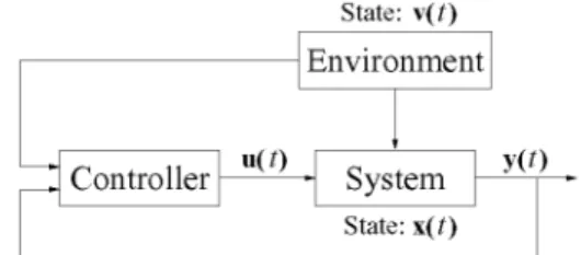
A control problem is often modeled by the in-teractions between the controller, the system, and the surrounding environment (see Fig. 1). Here, vector x(t) represents the internal state of the system at timet,v(t)is the environment
state,u(t)denotes the control signal, andy(t)is the output from the system.
Fig. 1.Model for controller, system, and environment.
The change in system state is usually modeled by a number of difference equations of the form:
xi(t+h)=xi(t)+∆xi(u x v t h) (1)
wherexiis thei-th system variable inx,∆xi()is the update function,tis the time,his the length of a time-step, and u, x, and vare the control signals, the system state, and the environment state of previous time-steps(sometimes several steps in the past). Real systems are often de-scribed by a set of non-linear differential equa-tions. In these cases, an approximation method, such as Runge-Kutta, is used as the update func-tion∆xi().
The online control strategy used here is called “direct control”4], in which the population en-codes the real-valued control signals . As men-tioned in the introduction, the control signals must be updated at certain intervals. Hence, only a limited number of evaluations is possible between updates of the control signals. How-ever, the number of evaluations(#ev)can be bal-anced between population size(ps)and number of generations(gen), i.e., #ev = ps gen. For instance, 200 evaluations can be assigned as ei-ther ps = 200,gen = 1 or ps = 25,gen = 8. Another important aspect of direct control is the control horizon(CH), which is used in the eval-uation of candidate solutions. The fitness of a solution is determined by its control perfor-mance forCH time-steps into the future. The best control setting is then used to control the real system for one time-step. In pseudocode, the direct control algorithm is as follows:
Direct control
Initialize population of sizeps
while(control period not over)f Reset best control setting
for(i=0;i<gen;i++)f Crossover and mutation
Evaluate each solution forCHsteps Selection
Store best control setting
g
Let best setting control one step
g
Direct control shares many properties with the control engineering approach known as gene-ralized predictive control(GPC)2]. However, GPC is not easily applied to non-linear prob-lems, because the determination of the con-trol signals, in this case, relies on minimization of a multimodal function, which is generally not possible with traditional engineering tech-niques.
3. The greenhouse control problem
The crop-producing greenhouse is modeled as illustrated in Fig. 1. The control, system, and environment variables are listed in Table 1.
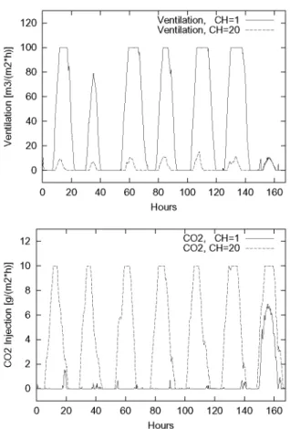
Table 1. Control, system, and environment variables in the greenhouse.
The greenhouse is controlled by four variables for heating(uheat), ventilation(uvent), injection of artificial CO2(uCO2), and injection of water
(uwater). The range of these control variables are as follows:uheat 20 150],uvent 20 100],
uCO2 2 0 10], and uwater 2 0 100]. The change in greenhouse state is modeled by six non-linear differential equations. The simulator is based on a German description7]. Unfortu-nately, the greenhouse simulator is too complex to describe in this paper, but a complete speci-fication in English is available in9].
The fitness of a solutionsat timetis calculated as the profit achieved, minus a penaltyp:
Fit(s t)= t+CH
X
j=t
∆xprof it(j);p(j) (2)
where
p(j)= 8
<
:
10 (16;xatemp(j)) xatemp(j)<16 10 (xatemp(j);35) xatemp(j)>35
0 otherwise
(3) The profit is equal to the income from the pro-duced crops minus the expenses for heating and CO2 (Eq. 29 in9]). The penalty is enforced to avoid damage to the crops and to ensure that the indoor air temperature is kept in the optimal range for growth.
Real weather data from the Aarslev measuring station on the island Fyn, Denmark, was used for the environment variables sunlight intensity
(vsun), outdoor air temperature(vatemp), outdoor ground temperature(vgtemp), relative humidity
(vRH), and wind speed (vwind). The remain-ing environemnt variables were kept constant to
scheme is to assume the weather to be fixed during the control horizon(few hours).
Fig. 2.Weather data for the first week of May.
4. Experiments and results
The simple EA encoded the four control signals as a real-valued vector. New solutions were cre-ated using Gaussian mutation and a variant of arithmetic crossover with one weight per vari-able. All weights except one were randomly assigned 0 or 1, and the remaining weight was set to a random value between 0 and 1. Binary tournament selection was applied. The algo-rithm used the following parameters: probabil-ity of crossover pc = 0:9, probability of muta-tion pm = 0:5, and variance σ = 0:01, which was scaled by the length of each control vari-able’s interval. Each solution was evaluated by simulatingCHtime-steps using the control set-ting encoded in the genome. The profit achieved in each step was recorded and used to calculate the fitness(Eq. 2).
Two sets of experiments were conducted. First, we investigated five trade-offs between popula-tion size and number of generapopula-tions. The trade-offs(ps gen) were(200, 1),(100, 2),(50, 4),
(25, 8), and (10, 20). Second, we tested six control horizons(CH) of 1, 2, 3, 4, 8, and 20 time-steps. Each experiment was repeated 30 times.
Fig. 3.Population size vs. generations. Control horizon of 4 steps. Average of 30 runs.
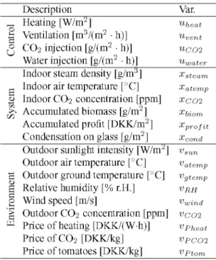
Fig. 4.Example of heating and CO2injection for best
control(upper graph)and worst control(lower graph)
Fig. 3 illustrates the profit per m2 in DKK for the five trade-offs using CH = 4. The graphs clearly show that the trade-off (10, 20) is the best. Furthermore, the order of the trade-offs shows an evident relationship between perfor-mance and number of generations – few gen-erations lead to low performance. Hence, the available evaluations are best utilized with a low population size and many generations between problem updates. In addition to the mentioned trade-offs, we obtained a near-optimal solution solution using 10000 evaluations with ps= 50 andgen = 200. The(10,20)-trade-off was, in fact, very close to the near-optimal solution. The control signalsuheat and uCO2for the best
setting(10, 20)and the worst(200, 1)are dis-played in Fig. 4. The difference in performance is closely related to these variables, because profit is easily lost on sub-optimal control of heating and CO2 injection. At night the
tem-peratures drop, which requires heating to avoid damage to the crops. At daytime the sunlight permits growth, which can be augmented by injection of additional CO2. The best control
strategy(Fig. 4, upper graph)properly adjusted the control to follow the day and night phases. The worst strategy failed to turn off heat at day-time, and valuable CO2 was wasted during the
night where no growth was possible because of the absent sunlight.
In the second set of experiments, we investi-gated the effect of varying the control horizon. We tested six horizons having 1, 2, 3, 4, 8, and 20 time-steps. Fig. 5 shows the results from the 1, 2, 4, and 20 horizons using the(10, 20) -trade-off(to keep the graph readable, 3 and 8 are not shown). A control horizon of 20 time-steps is
Fig. 5.Profit per m2for different control horizons with
10 individuals and 20 generations. Average of 30 runs.
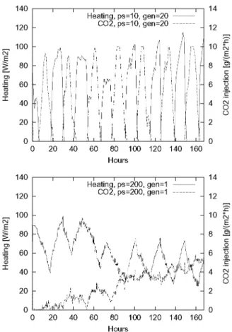
Fig. 6.Example of ventilation and CO2injection for
different control horizons(10 individuals, 20
generations).
the best, though only marginally better than a horizon of 8 steps. The profit achieved in the remaining four horizon decreases according to the look-ahead. Hence, a control horizon of at least 8 steps yields high profit, a horizon of 4 steps leads to a reasonably good profit, and only a few steps give rather low profit. The expla-nation for the significant difference between the worst performing setting(CH=1)and the best setting(CH = 20)is found by examining the control signals.
Fig. 6 displays ventilation(uvent) and CO2 in-jection(uCO2)forCH =1 andCH = 20. The graph on ventilation shows that two general con-trol strategies exist. The first strategy is used
when CH = 1. Here, the EA sets ventilation
high at daytime. This will require large invest-ment in heating during night, but will utilize the free CO2 in the environment better. The
second strategy appears when CH = 20. In
this strategy, ventilation is low, which saves some heating, but makes CO2 injection
20-step controller is mainly related to the achieved temperature and indoor CO2 level (Eq. 25 in
9]), which can be seen by thoroughly exam-ining the control signals and greenhouse states of both settings. Naturally, the two different control strategies emerge as a result of the con-trol horizon, but here the CO2 level plays an
important role too. The second strategy ap-pears because the long look-ahead allows the controller to discover the long-term effect of growth, i.e., that the photosynthesis can trans-form more CO2 than achievable by ventilation
alone. Hence, additional growth is possible by injecting artificial CO2. The short look-ahead
of the first strategy does not allow the controller to discover the long-term effects. Thus, venti-lation is used because it will provide free CO2
from the environment.
5. Discussion and conclusions
In this paper, we investigated two important as-pects of direct control with evolutionary algo-rithms. Our experiments show that the available number of evaluations is best invested using a low population size and many generations be-tween updates of the problem. Applying this re-sult essentially turns the dynamic problem into a series of related static problems. For instance, the combination of 10 individuals and 20 gener-ations performs significantly better than a popu-lation of 25 individuals and 8 generations. This is surprising because a population of 10 individ-uals is generally considered to be insufficient for most static problems. Interestingly, a long static period(20-50 generations)between prob-lem updates has been the preferred setting in most investigations on artificial dynamic prob-lems. Furthermore, this observation confirms the preliminary results obtained from an ear-lier investigation conducted by the first author of this paper 8]. Regarding future work, the general trend in the trade-off experiments sug-gests to test even more extreme settings. In this context, a comparison with other optimization techniques, such as particle swarm optimization and simulated annealing, may be in place. Our second series of experiments underlined the importance of choosing an appropriate control horizon. Interestingly, two very different con-trol strategies emerged. The first strategy settled
on high ventilation, much heating, low CO2
in-jection, and low water injection. This strategy occurred when the control horizon was short
(one time-step). The second strategy was nearly the opposite, i.e., low ventilation, medium heat-ing, high CO2 injection, and high water
injec-tion. This rather surprising difference is re-lated to the long-term effects of growth, such
as the CO2-consumption by the plants. A
control horizon of only one step does not re-veal this, because the indoor CO2 level does
not drop drastically from one step to the next. Hence, high ventilation gives free CO2 from
the environment, which is cheaper than aug-menting it artificially. An interesting question to ask in this context is would it be possible to switch to the better second strategy during the day? A possible answer is that the control setting corresponding to strategy two is more or less the opposite of strategy one. Hence, a switch would require a “jump” from one end of the search space to the other. Furthermore, following strategy one for a number of steps may actually render strategy two less profitable, because the search itself changes the problem; hence, the greenhouse state could be different. In a theoretical EA-context, this suggests mul-tiple optima intime rather than in space. Fur-ther analysis of the greenhouse state and control traces may shed some light on these matters.
Acknowledgements
This work was supported by the Slovenian Min-istry of Education, Science and Sport(project “Evolutionary Optimization of Dynamic Sys-tems”)and the Danish Research Council( EVA-Life project).
References
1] BRANKEJ., Evolutionary Approaches to Dynamic
Optimization Problems – Updated Survey. In: GECCO workshop on Evolutionary Algorithms for Dynamic Optimization Problems; 2001, pp. 27–30.
2] CLARKED.W., MOHTADIC., TUFFSP.S.,
General-ized Predictive Control – Part I. The Basic Algo-rithm,Automatica; 1987 23(2):137–148.
3] FILIPICˇ B., JURICIˇC´ D., An Interactive Genetic
Al-gorithm for Controller Parameter Optimization. In: R. F. Albrecht et al. (Eds.), Proc. of the
4] FOGARTYT.C., VAVAKF., CHENGP., Use of the
Ge-netic Algorithm for Load Balancing of Sugar Beet Presses. In: L. Eshelman(Ed.),Proc. of the Sixth
International Conference on Genetic Algorithms; 1995, pp. 617–624.
5] HUANGW., LAMH.N., Using Genetic Algorithms to
Optimize Controller Parameters for HVAC Systems, Energy Build; 1997, 26(3):277–282.
6] KRINK T., URSEM R.K., FILIPICˇ B., Evolutionary
Algorithms in Control Optimization: The Green-house Problem. In: L. Spector et al.(Eds.), Proc.
of the third Genetic and Evolutionary Computation Conference(GECCO-2001); 2001, pp. 440–447.
7] POHLHEIMH., HEIßNERA., Optimale Steuerung des
Klimas im Gew¨achshaus mit Evolution¨aren Algo-rithmen: Grundlagen, Verfahren und Ergebnisse, Techincal report, Technische Universit¨at Ilmenau; 1996.
8] URSEMR.K., Multinational GAs: Multimodal
Op-timization Techniques in Dynamic Environments. In: Proc. of the Second Genetic and Evolutionary Computation Conference (GECCO-2000); 2000,
pp. 19–26.
9] URSEM R.K., KRINK T., FILIPICˇ B., A
Numeri-cal Simulator of a Crop-Producing Greenhouse, Techincal report no. 2002-01, EVALife, Dept. of Computer Science, University of Aarhus; 2002.
www.evalife.dk
10] URSEM R.K., KRINK T., JENSEN M.T.,
MICHALEWICZZ., Analysis and Modeling of Con-trol Tasks in Dynamic Systems,IEEE Transactions on Evolutionary Computation6(4):378–389.
Received:June, 2002 Accepted:September, 2002
Contact address: Rasmus K. Ursem EVALife Research Group Dept. of Computer Science University of Aarhus Bldg. 540, Ny Munkegade DK-8000 Aarhus C, Denmark e-mail:[email protected]
Bogdan Filipicˇ
Dept. of Intelligent Systems “Jozef Stefan” Instituteˇ
Jamova 39 SI-1000 Ljubljana, Slovenia e-mail:[email protected]
Thiemo Krink EVALife Research Group Dept. of Computer Science University of Aarhus Bldg. 540, Ny Munkegade DK-8000 Aarhus C, Denmark e-mail:[email protected]
RASMUSK. URSEMinitiated his studies in computer science and mathe-matics in 1995 at the Dept. of Computer Science, University of Aarhus, Denmark. In 1997, he completed his minor in mathematics and started to focus on computer science in his MSc studies. Two years later, he started as a PhD student in the EVALife project under the special PhD programme at the Dept. of Computer Science, University of Aarhus, Denmark. He received his MSc degree in June 2001 and is currently working on his PhD thesis, which will be submitted in June 2003. The main focus in his PhD project is to develop novel evolutionary algo-rithms and to apply them to industrial problems in control engineering, in particular system identification and control of nonlinear dynamic systems. This work has mainly been published in the IEEE Transac-tions on Evolutionary Computation, the Proceedings of the Congress on Evolutionary Computation, and the Proceedings of the Genetic and Evolutionary Computation Conference.
In addition to this work, he has participated in the organization of EVAL-ife’s yearly workshop, he is in the program comittee of the Congress on Evolutionary Computation, and he co-lectures in EVALife’s course “Topics of Evolutionary Computation”.
BOGDANFILIPICˇreceived his PhD in computer science from the
Uni-versity of Ljubljana, Slovenia, in 1993. He is currently a Research Associate at the Department of Intelligent Systems of the “Jozef Ste-ˇ
fan” Institute, Ljubljana, and an Assistant Professor of computer and information science at the University of Ljubljana.
His research interests include evolutionary computing, intelligent data analysis and knowledge-based systems. He participates in research projects funded by the Slovenian Ministry of Science and Technology and by the European Commission, and in industrial projects dealing with resource optimization in production processes, such as continuous casting of steel and automobile production. He has published in sev-eral scientific journals, including IEEE Transactions on Systems, Man and Cybernetics, Engineering Applications of Artificial Intelligence, Computers in Industry, Review of Scientific Instruments, International Journal on Human-Computer Studies, and Applied Soft Computing. Dr. Filipiˇc is a member of the editorial boards of Applied Intelligence and the Journal of Computing and Information Technology, and serves as a programme committee member for the Genetic and Evolutionary Computation Conference(GECCO)and Parallel Problem Solving from
Nature(PPSN)conference.
THIEMOKRINKwas trained as a computer scientist(MSc)at the
Uni-versities of Erlangen and Hamburg, Germany(1988-1994). As a MSc
student, he worked on animal behaviour modelling in collaboration with biologists at the Dept. of Zoology in Oxford, UK. He continued his re-search at the Institute of Biological Science at the University of Aarhus, Denmark, where he received his PhD degree in 1997. Afterwards, he became Research Assistant Professor of biology at the University of Aarhus. In 1998/1999, he was employed as Research Assistant