Multi-Objective Artificial Bee Colony Algorithms and Chaotic-TOPSIS Method for Solving Flowshop Scheduling Problem and Decision Making

(1)

Multi-Objective Artificial Bee Colony Algorithms and

Chaotic-TOPSIS Method for Solving Flowshop Scheduling Problem and

Decision Making

Monalisa Panda

Department of Computer Science and Information Technology, Siksha ‘O’ Anusandhan Deemed to be University Bhubaneswar, 751030, Odisha, India

E-mail: [email protected]

Satchidananda Dehuri

Department of Information and Communication Technology, Fakir Mohan University Vyasa Vihar, Balasore, 756019, Odisha, India

Alok Kumar Jagadev

School of Computer Engineering, KIIT Deemed to be University Bhubaneswar, 751024, Odisha, India

Keywords: flowshop scheduling, multi-objective optimization, local search algorithms, artificial bee colony algorithm, multi-criteria decision making, chaotic-TOPSIS.

Received: December 13, 2018

Retrieval of optimal solution(s) for a Permutation Flow-Shop Scheduling Problem (PFSSP) within a reasonable computational timeframe has been a challenge till yet. The problem includes optimization of various criteria like makespan, total flowtime, earliness, tardiness, etc for obtaining a set of Pareto solutions in the process of Multi-Objective Optimization (MOO). This paper remodels a Discrete Artificial Bee Colony Algorithm (DABC) from a single objective optimization method to a multi- objective optimization one to solve the PFSSP executed and explored through the alternative and combined use of two local search algorithms named as: Iterated Greedy Search Algorithm (IGRS) and Iterated Local Search Algorithm (ILS). The algorithm has been classified into three different scenarios raised with the analysis of time complexity measure of applied local search methods prioritized through the insertion and swap operation of neighborhood structures that intensifies the local optima in the search space. The results of the DABC algorithm are summarized with respect to Total Completion Time (TCT), Mean Weighted Tardiness (MWT), and Mean Weighted Earliness (MWE). Based on the time complexity measure of the obtained results a Multi-Objective Artificial Bee Colony Algorithm (MOABC) has been proposed by adopting the simplest local search method of all in order to reflect the enhanced version of previously remodeled DABC algorithm. Finally, we propose a Chaotic based Technique for Order of Preference by Similarity to Ideal Solution (Chaotic-TOPSIS) using a suitable chaotic map for criteria adaptation in order to enhance the decision accuracy in the multi-Criteria Decision Making (MCDM) domain.

Povzetek: Članek se ukvarja z NP problemom večkriterijske optimizacije izdelave urnika z imenom Permutation Flow-Shop Scheduling Problem (PFSSP). Uvede Multi-Objective Artificial Bee Colony Algorithm (MOABC), tj. več-kriterijski algoritem z umetno čebeljo kolonijo in pokaže izboljšane rezultate.

1 Introduction and related work

The flowshop scheduling problem (FSSP) is a combinatorial optimization problem, inheriting the ideas from Barkers sequencing problem [1] that is based on ordering of jobs to determine a schedule. However, the problem is NP-hard and introduced by Johnson in 1954 [2]. It has a wide application in logistic, industrial, and many other fields. It aims to find the minimal total flow time (TFT) or total completion time (TCT) execution. The permutation flowshop scheduling problem (PFSSP)

(2)

specific moment on a single machine. When a machine is not available, automatically the jobs remaining are queued to a waiting state. An ongoing job, in a machine is not interrupted till completion.

During the last decades, the research attention for combinatorial optimization has turned to hybrid systems. It is observed that combination of different features from various optimization heuristics results in more robust and unique combinatorial optimization tools. Since the pioneering work of Johnson [2], a number of heuristics have been approached for solving FSSP. These proposed heuristics can be specified either as constructive or improvement. Most constructive heuristics [3-7] are the extended version of the Johnson’s algorithm [2], based on two or three-machine flowshop problems. In his work Palmer [3] developed a slope order index for sequencing the jobs with some allotted machines and processing times. A little variation to Palmer’s algorithm was proposed by Gupta [4] in order to estimate the same slope index. Also a lot many variants of branch and bound algorithms were developed subsequently [8-11] in this regard. Ignall and Scharge [10] applied the branch and bound scheme for the first time, based on two lower bounds in the two-machine FSSP. Bansal [8] extended the proposed idea to an m-machine case.

Due to the essence of optimizing multiple objectives in PFSSP, it is also extended to the multi-objective domain with many challenging approaches (non-heuristic and meta-heuristic). Selen and Hotts [12]solved a multi-objective flowshop scheduling problem (MOPFSSP) with m-machines by formulating a mixed-integer goal programming model with two objectives that is makespan and mean flowtime. Wilson [13] proposed an alternative model for it, by considering a fewer number of variables but at the same time he has added large number of constraints to it. Both the models have included same number of integer variables. Daniels and Chambers [14] proposed a branch and bound approach with two objectives (makespan and maximum tardiness) where they computed the Pareto solution for a 2-machine flowshop scheduling problem. Rajendran [15] also presented a similar procedure along with two heuristic approaches for the 2-machine flowshop scheduling problem with two objectives: minimization of TFT subject to optimal makespan. Similarly two different methodologies (one is based on a Branch and Bound (B&B) technique of exact algorithms and other one is based on Palmer approach of heuristic algorithms) are used [16] to find the optimum solution for minimization of bi-criterion (makespan, weighted mean flowtime) objective function of three machines FSSP with transportation times and weight of the jobs. Recently a production scheduling problem in hybrid shops has been solved by Mousavi et al.[17], by assuming some realistic assumptions.

Like the non-heuristics, many meta-heuristic methods like trajectory based and population based methods have also been proposed to solve MOPFSSPs. Chakravarthy and Rajendran [18] proposed a simulated annealing (SA) algorithm for resolving the m-machine FSSP to minimize makespan and maximum tardiness.

Similarly many SA algorithms [19-21] were proposed to optimize various objectives like makespan, TFT, and total tardiness. Another SA algorithm was approached by Loukil et al. [22] based on m-machine case. The algorithm assumed objective pairs out of a number of objectives such as: average weighted completion time, makespan, average weighted tardiness, maximum earliness, maximum tardiness, and the number of tardy jobs. A novel multi-objective memetic search algorithm (MMSA) [23] is proposed to solve the MOPFSSP with makespan and total flowtime. The performance of the algorithm is validated and compared with the four state-of-the-art algorithms on a number of benchmark problem and provides better solutions than these compared algorithms. Another novel fuzzy multi-objective local search-based decomposition algorithm has been approached for solving a fuzzy-MOPFSSP for two fuzzy objectives, that is, the fuzzy makespan and the fuzzy total flow time. An extensive computational study on Taillard benchmarks has been conducted to compare the proposed algorithm with the fuzzy NSGAII and the results demonstrate the effectiveness of the proposed algorithm [24].

Among meta-heuristics, swarm intelligence has created a class of its own, which models the collective behavior of self-organized models and applies these models to solve many complex problems. Earlier works have adopted ant colony optimization (ACO) and particle swarm optimization (PSO) algorithms to simulate the swarm behavior of ant colonies and flocks of birds, respectively. There are a few researches which implements the PSO and ACO for solving the MOPFSSP [25-29] subject to makespan, TFT and completion time variance. Recently, a lot many algorithms have been proposed by modeling the intelligent behaviors of real bee swarms in this regard. The emerging research with artificial bee colony algorithms (ABC) demonstrates that these algorithms outperform and is equally competitive as compared to other population-based algorithms with the advantage of employing fewer control parameters [30-35]. Sharma et al. [36] provided a state art survey of ABC algorithm and its performance analysis with different size of population. Singh [37] has explained how one can solve different optimization problems using ABC algorithm. Recently, Amlan et al.[38] applied a Regional Flood Frequency Analysis (RFFA) to 33 stream gauging stations in the Eastern Black Sea Basin, Turkey. Tereshko [39] proposed a DABC algorithm for the FSSP with intermediate buffers (IBFSP) in order to minimize the maximum completion time. The DABC algorithm uses the effectiveness of the insertion and swap operators to produce neighbourhood solutions at the employed bee phase. From many such articles [40-42] it is clearly understood that, swarm intelligence provides a better algorithmic framework inspired by the intelligent behaviour of the animals, birds and social insects.

(3)

complexity of the algorithm. To deal with this, we have remodelled the DABC algorithm of Tasgetiren et al.[43] for three different cases by the application of some effective strategies. The proposed algorithm is inherited with the hybridization of swap/insertion operations and

construction-destruction procedures for the neighbourhood structures known as iterated local search

(ILS) and iterated greedy search algorithm (IGRS) respectively. Through an experimental analysis, the proposed algorithmic cases are evaluated for best CPU time utilization with respect to three objectives such as: TCT, weighted mean tardiness (WMT), and weighted mean earliness (WME). Again in the same scenario we have tested the results of canonical ABC against DABC algorithm. Genuinely due to multiple objectives, here ABC has been turned to multi-objective ABC (MOABC) with necessary improvements to solve the MOPFSSP.

While working with multiple-objectives it is almost impossible to get a single compromising solution. The situation leads to a multi-criteria decision making (MCDM) scenario. MCDM is the most powerful branch of decision making: generally handles multiple objective functions together and includes a lot many approaches that have been applied to different problem domains to choose the best alternative. But major parameters like criterion weight in these methods are founded on randomness of data. Mareschal [44] has claimed that proper weight assignment to each criterion will lead to a better and more appropriate decision making framework for both qualitative and quantitative data. However, the weight assignment procedure (specifically to qualitative criteria) is completely dependent upon the decision maker’s preference and varies remarkably from one decision maker to other. This paper proposes TOPSIS using chaotic maps for generating random numbers during criteria adaptation to improve the decision accuracy. The chaotic number generators emerges a random number each time when needed by the decision maker to define the criterion weight. To maintain the criterion preference, we have sorted the random numbers and assigned them accordingly.

The remaining parts of the paper are assembled as follows. Section 2 presents the problem formulation and assumptions. The canonical ABC and DABC algorithm has been illustrated in Sections 3 and 4 and Section 4

also represents the details of the ILS algorithm and IGRS algorithm applied in MOPFSSP. Section 5 encloses the multi-objective ABC for PFSSP. Section 6 contains the computational results for both algorithms with two different synthetic datasets. Decision making using chaotic-TOPSIS is illustrated in section 7. Section 8 concludes the article with future directions.

2 Problem description and

assumptions

A PFSSP is consisting of n jobs (ᴨ1, ᴨ2, ᴨ3... ᴨn), each

having m number of tasks, that have to be processed in separate machines. A schedule for the jobs is the assignment of tasks to time intervals on the available machines. Task Tji must be assigned to machine j where

the task belongs to job i, additionally for any job i, the processing of task Tji cannot be started till Tji-1 has been

completed. Where,

i ϵ(1, n) and j ϵ(1, m).

Ojk = processing time of job j on machine k. Assumptions

(i) Jobs consist of a pre-ordered sequence of operations.

(ii) At a time only one job can be processed on one machine.

(iii) The job orderings are same for all machines. (iv) Timeslot of different job operations is

predetermined.

(v) Once a job starts being processed on the first machine, cannot be interrupted in between either on or between machines.

(vi) Release time of all jobs is zero.

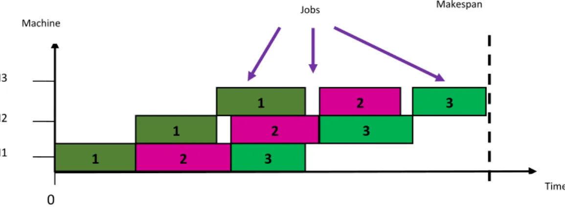
As per above stated assumptions, a dummy PFSSP; having ‘3’ jobs, each with ‘3’ operations having some random processing time can be executed in ‘3’ different machines as follows:

With regard to the above context: F (ᴨj), the

flowtime of job ᴨjis same as the completion time C (ᴨj, m) on the machine m. So the total completion time (TCT

(ᴨ)) of all jobs is equal to maximum of flow time or completion time of all jobs and is calculated as:

Figure 1: A dummy PFSSP.

Machine

M3

M2

M1 ₁ ₂ ₃

1 2 3

Jobs Makespan

(4)

) 1 ( ) , ( max ) ( max ) (

1 1



= =

=

= n

j

n j

j

j C m

F

TCT   

Similarly let Dj, be the due date and Cj the

completion time of job j, for jϵn. The jobs earliness and tardiness can be computed by, Ej=max {Dj-Cj, 0} and Tj=max {Cj-Dj, 0} respectively. Hence the weighted

mean tardiness and weighted mean earliness of different job sequence can be calculated as:

) 2 ( ]

0 ; max[

1 1



=

= −

= _n

j j n

j j j j

e

e e C D WME

) 3 ( ]

0 ; max[

1 1



=

= −

=

n j j n

j j j j

R

r r D C WMT

where,

n

=number of jobs

j

=job index

j

D =due date of job j. j

C = completion time of job j. j

A

=arrival time of job j in the shop.

j

e

= earliness cost per unit time for job j

j

r

=tardiness of job j penalty per unit time.

3 Canonical ABC algorithm

ABC, a member of swarm intelligence is a meta-heuristic algorithm based on the intelligent behavior of honey bees, introduced by Karaboga [30, 34-35, 45]. Due to its simplicity and good performance reported in various fields while optimizing both single and multi-objective problem, we motivated to extend its usage in PFSSP. It is inspired by the nature that is by the foraging behavior of real honey bees, their self-organization capability, and specially division of labor features. The canonical ABC algorithm has some essential components like food sources, nectar-amount in each source, and three kinds of foraging honey bees (employed bee, onlooker bee, and scout bee). Here every food source signifies a candidate solution in the search space and the fitness of these solutions is equivalent to the nectar-amount of those food sources. Employed bees go on searching random food positions; they also share the collected information about food sources among the onlooker bees through the waggle dance. Onlooker bees select the better sources (better solutions) with high nectar amount (high fitness value), based on the information (fitness value) from the employed bees. Scout bees are those employed bees which could not found remarkable food sources. The pseudo-code of canonical ABC is given below.

Initialize population (P)

Fitness evaluation (fi) {

While (cycle<=maximum number of cycle) {

Employed bee phase

{

Produce neighborhoods Fitness evaluation selection (fi)

Probability calculation (pi)

}

Onlooker bee phase

{

Select a solution based on probability pi Produce new solution

Fitness evaluation

Greedy selection procedure

}

Scout bee phase

{

Replace the abandoned one

}

Memorize the best

cycle++

}

4 Modified discrete artificial bee

colony algorithm

Though ABC algorithm is a proved continuous optimizer for various combinatorial optimization problems, later has also shown its efficiency towards discrete version of it. Here, we use a modified version of the above ABC algorithm to handle discrete decision variables. We have extended the single objective problem of Tasgetiren et al. [43] to a multi-objective one and the detailed of modified DABC has been discussed below:

Initialization:

The population is initialized with a random set of solutions, each consisting with a random permutation of jobs.

ᴨ = (ᴨ1, ᴨ2, ᴨ3... ᴨn) (4)

Employed bee phase:

According to the basic ABC algorithm, the employed bees generate their neighborhood nectar sources. Here for obtaining the nearer food sources, we will take the advantage of the adopted strategies from IG_RS algorithm and ILS [43]. From IG_RS algorithm we have borrowed the concept of construction and destruction

procedure and the two common operators named insert

(5)

separately as DABC-I, DABC-II and DABC-III respectively. This step attempts to improve the population deterministically by accepting the improved adjacent solutions by examining their fitness values. The solutions to next step are chosen on the basis of equal number of best solutions from each objective respectively to maintain the population diversity.

Case I:

Each nearest solution in the population is determined by any one of the following strategy. The selected strategy is applied two times separately to each permutation ᴨ in the population, resulting two nearest neighbors and the best one is selected to the next step.

(i) Applying two-insert moves to a permutation ᴨ with p=2.

(ii) Applying three-insert moves to a permutation ᴨ with p=3.

(iii) Applying two-swap moves to a permutation ᴨ with p=2.

(iv) Applying three-swap moves to a permutation ᴨ with p=3.

Case II:

Each nearest solution is chosen by applying any of the following strategy.

(i) Applying two-insert moves to a permutation ᴨ with p=2.

(ii) Applying three-insert moves to a permutation ᴨ with p=3.

(iii) Applying two-swap moves to a permutation ᴨ with p=2.

(iv) Applying three-swap moves to a permutation ᴨ with p=3.

(v) Applying one destruct-construct procedure to a permutation ᴨ with destruction size x.

Case III:

The nearest solutions are determined by using the following strategy.

(i) Applying destruct-construct procedure to a permutation ᴨ withdestruction size x.

Onlooker bee phase:

This phase selects a food source based on the probabilities obtained from the fitness values during employed bee phase. The aim of this phase is to find further better compromising solutions by applying well devised local search. The probabilistic selection can be described as: ) 5 (



= j j i i fit fit p

Here fiti is defined as the fitness value of the ith

solution compared to other solutions in the solution set. The solutions with a higher probability are always selected to the next cycle.In addition to this, almost an equivalent strategy to that of employed bee phase is employed during the onlooker bee phase to produce a new neighborhood solution. An efficient local search method has to be applied to further improve the candidates of the onlooker bee phase. A better food

source has to replace the current one and become a new member in the population; else both are treated as non-dominated to each other.

Scout phase:

In general, the scout bee phase removes the abandoned solutions (worst solutions) from the search space and tries to discover new ones with better fitness value. Therefore, the DABC algorithm removes a defined number of worst solutions and replaces them with new ones by the process of tournament selection in order to deal with local optima by avoiding the trial counter.

During the evolution process, the solutions will be prioritised with respect to TCT, WMT and WME. Also the different cases of the employed bee phase will fall to different CPU utilization of the algorithm. As per the selection of basic ABC algorithm, an old solution is replaced by a new one if it is found to be superior in all objectives by using a greedy selection procedure.

A common framework for DABC-I, DABC-II, and DABC-III as follows:

)

(

)

...

,...

,

(

]

[

)

,

(

)

1 (

)

(

_

)

1 (

]

ker

[

)

,

(

)

1 (

)

(

_

)

1 (

]

[

)

(

)

1 (

]

[

...

,...

,

]

[

3 2 1 3 2 1



return

solutions

abandoned

replace

for

phase

bee

Scout

sequence

best

ate

propertion

M

to

objetive

for

search

local

N

to

i

for

phase

bee

onloo

sequence

best

ate

propertion

M

to

objetive

for

search

local

N

to

i

for

phase

bee

Employed

f

Calculate

N

to

i

for

n

calculatio

Fitness

tion

Initializa

N new new new new i N

=

−

=

−

=

Figure 2: DABC algorithm

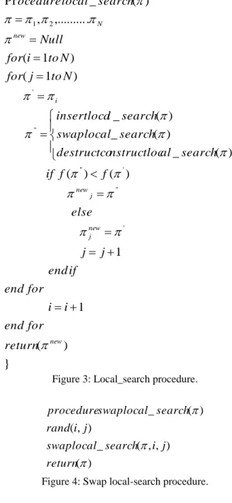
4.1 Local search methods: IG_RS

algorithm and ILS algorithm

(6)

algorithm reconstructs a job pool by assigning best positions to a sub part of the original job sequence. Here the destruction phase randomly removes x number of jobs from the permutation ᴨ without repetition resulting two partial solutions ᴨx(x number of jobs) and ᴨx’ (x’=n-x

number of jobs). Then the construction phase adds each removed jobs back to the pool in the same order by searching its best position. The motivation of using the above methodologies in our algorithm is inherited from the efficacy of the DABC algorithm. Here the focused parameters are: perturbation strength p and the

destruction size x that has to be carefully chosen. A perturbation is achieved by a random insertion of a job to another position or by swapping of some jobs randomly in a permutation ᴨ. Similarly choosing a larger destruction size for x will lead to a better result and a smaller one will be good for CPU time minimization. Tasgetiren et al. [43] have considered the perturbation values are as 1or 2 and the x values as 8 or 12 for different instances of Taillard [46]. However in our work, we have considered two synthetic datasets for small and large sized systems with variable number of jobs and machines. Here the p values are considered as 2 or 3 and the x values are considered as 2 (for small sized) and 4 (for large size) respectively.

5 MOABC for MOPFSSP

The above proposed DABC algorithm is the direct extension of single objective DABC proposed by Tasgetiren et al. [43]. The algorithmic framework and search for local optima is much more flexible and effective with the advantages of local search algorithms in the DABC algorithm. To achieve a more accurate and efficient problem solving approach in the field of multi objective optimization; we have simulated these advantages to model a multi objective Pareto-based ABC algorithm with same objectives to solve the FSSP. The proposed MOABC algorithm combines the main idea of ABC with the above local search strategy to search the neighborhood structure. To apply the local search algorithm in the next proposed one, we have adopted one of the simpler one i.e., the swap () local-search instead of using all methods randomly. Firstly the proposed MOABC algorithm initiates a number of randomized job sequences of n jobs, and is stored in the population matrix. These sequences represent the random food sources of ABC, with certain quality and diversity. Secondly, an exploitation search procedure for the first two bee phases (employed and onlooker) is designed to best suit the problem and to intensify the local search operation. To record the updated non-dominated sequence emerged in each cycle, it uses a Pareto-based

}

)

(

1

1 )

(

)

(

)

(

_

)

(

_

)

(

_

)

1 (

)

1 (

.

,...

,

)

(

_

Pr

' '' ' '' '' ' 2 1 new new j j new i new N

return

for

end

i

for

end

if

end

j

else

f

if

search

al

nstructloc

destructco

search

swaplocal

search

l

insertloca

N

to

j

for

N

to

i

for

Null

search

local

ocedure



+

=

+

=













=

Figure 3: Local_search procedure.

)

(

)

,

(

_

)

,

(

)

(

_



return

j

i

search

swaplocal

j

i

rand

search

swaplocal

procedure

Figure 4: Swap local-search procedure.

procedure

end

return

j

i

insert

j

i

rand

search

l

insertloca

procedure

)

(

)

,

(

)

,

(

)

(

_



Figure 5: Insert local_search procedure.

procedure

end

return

construct

destruct

d

nstruct

destructco

procedure

R D d R D

)

(

)

,

(

)

(

)

,

(



=

(7)

archive set. In addition, the population is well-adjusted to maintain diversity in scout bee phase by eliminating the worst solutions. It is seen that proposed algorithm is able to find the best set of solutions and a proper statistical analysis has also been done to evaluate the proposed algorithm’s performance with different inputs. Some important terms related to MOABC can be defined below.

Pareto dominance

Any solution S′ is said to be non-dominated to S′′ if and only if,

(i) (i)The solution S′ is no worse than S′′ in all the objectives.

(ii) The solution S′ is strictly better than S′′ in at least one objective.

Pareto optimal solution set and Pareto optimal front

Pareto optimal solution set is the group of all Pareto optimal solutions, and the respective graphical representation in the objective space is known as the Pareto optimal front.

Archive

An archive records the track of the non-dominated solutions from time to time. It is iteratively updated throughout the search procedure. Once a new non-dominated solution generated, the archive is updated accordingly.

5.1 Problem formulation

The FSSP is rescheduled (fixed to similar assumptions as stated above) with the same three defined criterions (TCT, WMT and WME) and n jobs to be solved with ABC. As we know mostly there will be multiple solutions, non-dominated to one another will be emerged during the simultaneous optimization of multiple objectives (known to discover true Pareto front), we have done a straight forward extension of uni-objective ABC as well as above DABC to redesign an MOABC algorithm. In the employed bee phase, an exploitation search procedure is applied on the initialized solutions, to derive the non-dominated solution set. The generated Pareto front is maintained in an archive with the corresponding trial counters and will be updated from time to time. Onlooker bees search for more intensified solutions within the neighborhood of the food source in their memory. Finally, the abandoned solutions are deleted from the archive to stand with a best fitted Pareto front.

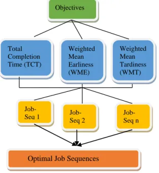
5.2 Architecture

As per the problem architecture, ‘n’ jobs are divided into

‘m’ number of tasks, to be sequenced differently and to

be processed in different machines. Each job sequences are evaluated through their fitness values against the individual objective functions. After the problem evaluation, the resulted sequences are listed out that are non-dominating to each other. Figure 7 is representing the MOPFSSP problem architecture which needs to be

optimized to a set of optimal job sequences as corresponding non- dominated set.

Figure 7: MOPFSSP architecture.

Figure 8 is represents the proposed solution strategy using MOABC. The proposed model generates multiple Pareto optimal solutions iteratively which are updated in an external archive time to time. Here the algorithm adopts the 2swap () local search strategy to generate the neighborhood structures in the solution space. The selection of the same local search procedure is based upon the time complexity analysis of all considered methods in the remodeled DABC algorithm.

5.3 Proposed MOABC

This section presents the algorithmic representation of proposed MOABC algorithm to solve MOPFSSP.

The derived MOABC algorithm, initializes the population ‘ᴨ’ with ‘n’ solutions, each consisting of a random number of job sequences similar to the DABC algorithm. Each updated solutions in the population matrix are evaluated for the corresponding fitness value using the objective functions 1- 3. The generated non-dominated set is maintained in an archive with the corresponding trial counters; which is updated in every cycle. Employed bees explore for better sources in the neighborhood by applying swap () operation, where two randomly selected jobs i and j (two random selected dimensions) for a random solution (sequence) k are

Objectives

Total Completion Time (TCT)

Weighted Mean Tardiness (WMT) Weighted

Mean Earliness (WME)

Job-Seq 2

Job-Seq n

Job-Seq 1

Optimal Job Sequences

Figure 8: Proposed framework using MOABC.

MOPFFS P

MOA BC algori thm

Hybridiza tion with 2-swap method

(8)

swapped with each other. Onlooker bee selects a candidate source depending on its probability values calculated and provided by the employed bees. The solutions with a greater probability are shifted to the archive. Within a defined number of cycles, the employed bees whose solutions cannot be further improved (through a predetermined number of trials) are treated as abandoned ones and are deleted permanently from the archive. These abandoned solutions are calculated by the help of trial counters. If a solution in S

is improved by the corresponding solution in S’ then the trial counter is set to zero (0), else it is set to one (1).

6 Numerical simulation

The numerical results represent the performance of both DABC algorithm and MOABC algorithm respectively with respect of TCT, WMEe_{and WMT}r_{. Two different}

datasets have been initialized with little parameter variation. One of this has been initialized with small processing times and due dates named as ‘small-size dataset’ and the other one is named as ‘large-size’. For

both the proposed algorithms, we have considered similar input datasets.

6.1 Control parameters

However both the algorithms require same control parameters except the case of abandoned solution. The DABC algorithm removes a defined number of worst solutions and replaces them with new ones in order to remove abandoned solutions from the population where as the MOABC algorithm removes those solutions based on a trial counter limit.

6.1.1 Parameters of DABC

Parameters: Values:

Population size 10

Maximum iterations 50

Number of onlookers 1/2*(colony size)

Number of employed bees 1/2*(colony size)

Worst solutions to be replaced 2 or 4

6.1.2 Parameters of MOABC

Parameters: Values:

Colony size 10

Maximum iterations 50

Number of onlookers 1/2*(colony size)

Number of employed bees 1/2*(colony size)

Limit for abandoned solution 20

6.2 Description of the numerical data

To evaluate DABC-I, DABC-II and DABC-III, two instances of datasets are customized with two different combinations of jobs and machines. With a little parameter variation both the datasets consider same population size of 10. The due date of each job is initialized separately with respect to two datasets. We have assigned same weight for both tardiness and earliness in both the input sets, while evaluating WMEe

and WMTr_{. Again the same datasets are used to}

characterise the performance of MOABC.

6.2.1 Small-size data

To validate the results at an eye, a small size dataset is randomized with a combination of 4 jobs and 3 machines with an ideal parameter setting. The processing time (Oik)

of the jobs are set within [0, 5] and the due times are set in [10, 15]. The earliness and tardiness weights are considered in the range [1, 10]. Based on the due time, the calculated TCT and the weights (earliness and tardiness), the MWT and MWE of the jobs have to be calculated. The destruction size has been assumed as 2. All these parameters, input data, corresponding statistics and the initial population sequence are tabulated below.

BEGIN

{

Set parameters; Set population size; Initialize solutions; Archive=Null; Trial counter=Null;

For each solution find the fitness value;

Generate the non-dominated set; Update Archive;

Do

{

//Employed bee phase//

Generate all employed bees and check their dominance relation to nearby solutions by swaplocal_ search procedure;

Compute the Fitness value; Compute non-dominated set; Update Archive;

Update trial counter; //Onlooker bee phase// Update the solutions using swaplocal_search () algorithm;

Compute the Fitness value; Compute non-dominated set; Update Archive;

Update trial counter;

} While (Stop criterion=Max. no. of iterations);

//Scout bee phase//

Delete abandoned solutions Update Archive;

}

END

(9)

Parameter setting

(i) Ojk :[1-5]

(ii) Weight (tardiness and earliness): [1, 10]

(iii) Population size: 10

(iv) Destruction size: 2

(v) Due time: [10, 15]

Table 1 represents the processing time of 4 different jobs with respect to 3 machines. Also it initializes the expected finish time of each job and an assigned weight which will be further used to calculate the fitness value of the defined objective functions.

Table 2 contains the statistical analysis of standard deviation for each job( small-sized dataset).To calculate the standard deviation we have summarized the minimum and maximum processing time of each job

from the pool. The result shows that, standard deviation of each job ranges between [0, 1].

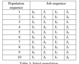
Using the above information a randomized job sequence is initialized with population size 10. As we have considered 4 jobs here, it can have 24 numbers of different possible sequences. Table 3 contains a random selection of 10 sequences out of these. These sequences will be the initial input for the proposed algorithm and the resulted intermediate sequences will be the further inputs for different iterations and bee phases.

6.2.2 Large-size data

The other synthetic large size dataset with population size 10 is generated with 10 jobs and 9 machines are set with the following parameter setting. Here the processing time of jobs are set to [0, 10]. The weights and due times

Job 1 Job 2 Job 3 Job 4

Machine 1 O11=4 O12=1 O13=5 O14=2

Machine 2 O21=3 O22=2 O23=4 O24=3

Machine 3 O31=5 O32=2 O33=3 O34=4

Due time 10 12 30 15

Weight 2 3 4 2

Table 1: Processing time of machine vs task of each job.

Jobs Minimum Maximum Standard deviation

1 3 5 0.81

2 1 2 0.47

3 3 5 0.81

4 2 4 0.81

Table 2: Statistics of the small-size dataset.

Population sequence

Job sequence

1 J0 J1 J2 J3

2 J1 J2 J3 J0

3 J2 J3 J0 J1

4 J3 J0 J1 J2

5 J3 J2 J1 J0

6 J0 J3 J2 J1

7 J1 J0 J3 J2

8 J2 J1 J0 J3

9 J0 J1 J2 J3

10 J1 J2 J3 J0

Table 3: Initial population.

Job 0 Job 1 Job

2

Job 3

Job 4

Job 5

Job 6

Job 7

Jo b 8

Job 9 Machine 1 O11=10 O12=5 O13=8 O14=5 O15=1 O16=7 O17=2 O18=0 O19=9 O1 10=3

Machine 2 O21=3 O22=4 O23=5 O24=8 O25=3 O26=6 O27=2 O28=5 O29=7 O2 10=4

Due time 80 42 75 85 95 60 10

0

10 5

9 0

65

Weight 2 3 4 6 10 1 4 5 7 9

(10)

are initialized within [1, 10] and [50, 100] respectively. The destruction size has been assumed as 4. The same required data as per the small sized dataset are also represented using different tabulations in the same sequence.

Parameter setting

(i) Ojk :[0-10]

(ii) Weight (tardiness and earliness): [1, 10]

(iii) Population size: 10

(iv) Destruction size: 4

As per the parameter setting, Table 4 is finalized with different processing times for individual jobs with respect to corresponding machines. It also assumes the due times and job weights. Job weights are basically the representative of their priorities.

Similar to the first dataset, we have also done a statistical analysis of the large-size dataset in Table 5.As per the minimum and maximum processing time of each job, the standard deviation of the jobs ranges between [1,3].

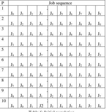
Table 6 contains the initial population set consisting of 10 jobs. These jobs can be arranged in 10! number of possible ways and we have selected a random 10 out of it

as the initial input. As compared to the small-sized dataset there is a very less chance of repeating the same sequences as the intermediate result sequences, due the application of different tuning operators

(insert/swap/construct-destruct).

6.3 Numerical results and analysis

Using the above specified inputs the results are tabulated separately for each algorithm. First, the results of DABC are represented and then that of MOABC. Firstly the results are tabulated then are reflected into corresponding graphical representations through the help of various figures where ‘X’ and ‘Y’ dimensions represents the ‘performance score’ versus ‘job sequences’ respectively. Each unit of ‘X’ and ‘Y’ dimension in the small-size dataset counts as 5 and 1 respectively, similarly it counts as 20 and 1 for the large- size dataset for the same dimensional sequence.

6.3.1 Results of DABC Algorithm

The tabulated results include the performance of DABC algorithms for individual cases with two specified inputs. Table 7-9 represents the final job sequences for small dataset corresponding to TCT, MWT and MWE and table 10-12 includes the results for the other input dataset. Table 7 and 10 includes the results of DABC-I algorithm with swap () and insert () operation having random perturbation values 2 or 3. Table 8 and 11 shows the results of DABC-II, that include another operation construct-destruct () additional to the operations of DABC-I. Only construct-destruct is used in DABC-III and the results are tabulated in Table 9 and12.

6.3.1.1 Small-size dataset

Table 7 contains the resulted TCT, MWT, MWE of the small-sized dataset for DABC-I. As mentioned, DABC-I uses the swap () and insert () algorithms to update the solution vectors. The result includes the completion time of every job in different sequences and TCT of each job sequence is equal to the completion time of the last job of the individual sequence. According to the initialized weight and due time the respective MWT and MWE has been calculated.

The graphical representation of Table 7 has been shown in Figure 10. Each job sequences have been represented individually with its corresponding TCT, MWE, and MWT scores.

The results of DABC-II is tabulated in Table 8.Based on the completion time, weight and due date of individual jobs the corresponding TCT, MWT, and MWE values are summarized and presented here. To update the job sequences here all the local search methods (insert/swap/construction and destruction) have been applied randomly.

Jobs Minimum Maximum Standard deviation

1 1 10 2.81

2 0 5 1.45

3 0 8 2.40

4 0 10 3.18

5 1 8 1.94

6 3 9 2.07

7 0 9 2.40

8 0 9 2.72

9 0 9 2.53

10 2 7 1.76

Table 5: Statistics of the large-size dataset.

P Job sequence

1 J

J0 J J1 J J2 J J3 J J4 J J5 J J6 J J7 J J8 J J9

2 J

3 J

4 J

5 J

6 J

7 J

8 J

9 J

10 J

J9 J J0 J J1 2 J2 J J3 J J4 J J5 J J6 J J7 J J8

(11)

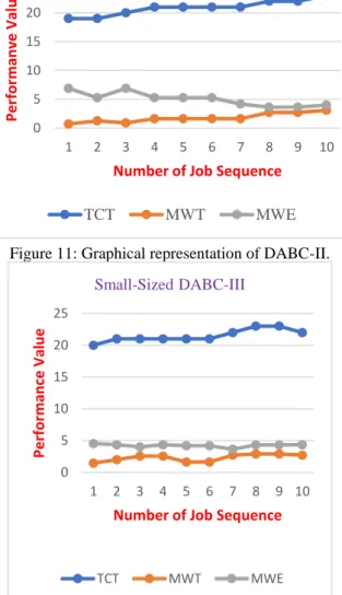
The tabulated results of DABC-II are graphically represented in Figure 11. Like DABC-I, most of the cases have more earliness penalty than the tardiness penalty. While adopting selection of average number of solution sequences from each objective, we found some of the repeating sequences. These have to be treated as one ultimately. Hence, the total numbers of non-dominated sequences are 7 in number but we have represented all repeated sequences also.

The results of DABC-III have been listed in Table 9. The three objective functions are evaluated with a recursive set of sequences and the fitness values are summarized. DABC-III explicitly uses destruct- construct for perturbing the solution sets.

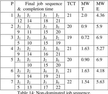
P Final job sequence &

completion time TC T

MW T

MWE

1 J3 J1 J0 J2 19 0.72 5.54

9 11 16 19

2 J3 J1 J2 J0 20 0.9 5.9

9 11 15 20

3 J0 J1 J3 J2 21 2.0 4.36

12 14 18 21

4 J1 J0 J2 J3 21 1.3 5.6

5 13 17 21

5 J1 J2 J0 J3 22 1.54 5.27

5 13 18 22

6 J1 J2 J3 J0 22 1.54 5.63

5 13 17 22

7 J2 J1 J0 J3 23 2.36 4.0 12 14 19 23

8 J0 J3 J2 J1 21 2.54 4.0 12 16 19 21

9 J0 J3 J1 J2 21 2.54 4.36 12 16 18 21

10 J2 J3 J1 J0 23 2.9 4.36 12 16 18 23

Table 7: Results of DABC-I.

Population Final job

sequence & completion time

TCT MWT MWE

1 J1 J3 J0 J2 19 0.72 6.9

5 10 15 19

2 J3 J0 J1 J2 19 1.27 5.27

9 14 16 19

3 J1 J3 J2 J0 20 0.90 6.9

5 10 15 20

4 J3 J2 J1 J0 21 1.63 5.27

9 14 16 21

5 J3 J2 J1 J0 21 1.63 5.27

9 14 16 21

6 J3 J2 J1 J0 21 1.63 5.27

9 14 16 21

7 J3 J2 J0 J1 21 1.63 4.18

9 14 19 21

8 J0 J2 J3 J1 22 2.72 3.63

12 16 20 22

9 J0 J2 J3 J1 22 2.72 3.63

12 16 20 22

10 J2 J0 J1 J3 23 3.18 4.0

12 17 19 23

Table 8: Results of DABC-II.

Figure 10 Graphical representation of DABC-I.

Figure 11: Graphical representation of DABC-II.

Figure 12: Graphical representation of DABC-III.

0 5 10 15 20 25

1 2 3 4 5 6 7 8 9 10

Per

for

m

an

ce

Val

u

e

Number of Job Sequence

Small-Sized DABC-I

TCT MWT MWE

0 5 10 15 20 25

1 2 3 4 5 6 7 8 9 10

Per

for

m

an

ve

Value

Small-Sized DABC-II

TCT MWT MWE

0 5 10 15 20 25

1 2 3 4 5 6 7 8 9 10

P

er

for

m

anc

e

Va

lu

e

Small-Sized DABC-III

(12)

Table 9 results are graphically represented in Figure 12 showing a clear-cut demarcation of TCT, MWE, and MWT for 10 different sequences. Apart from TCT, most of the non-dominated sequences have earliness penalty is more than tardiness penalty.

6.3.1.2 Large-size dataset

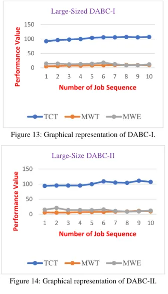
Table 10 stores the results of DABC-I for the large-sized dataset. Along with every sequence, the completion time of individual jobs are listed leading to the TCT score of that sequence. Out of 10 random sequences of 10 different jobs, 8 sequences are having greater MWE score than MWT.

Table 10 is graphically represented in Figure 13, showing the ratio of MWE score, MWT score, and TMT score of individual job sequence. Except sequence 10 and 9, other sequences are having more MWE score than MWT score.

Results of DABC-II for the second input are stored in Table 11. The results also show similar efficiency as that before. Here also the earliness cost is more in many sequences.

Figure 14 represents Table 11. We can obtain the better sequences having minimum TCT, MWT, and MWE. As discussed, DABC-II uses all the local search methods to improve pre existing solutions.

DABC-III results for the large-sized input are tabulated in Table 12. It shows construct-destruct () has similar efficiency to search good solutions from the search space. But, out of all local search algorithms this one is having maximum algorithmic complexity.

Figure 15 represents DABC-III, pictorially showing the fitness value of different resulted sequences.

As discussed above the result tables and corresponding graphs have been represented below.

P Final job sequence &

completion time TC T

M WT

M WE

1 J3 J0 J2 J1 20 1.45 4.54

9 14 18 20

2 J0 J1 J3 J2 21 2.0 4.36

12 14 18 21

3 J0 J3 J2 J1 21 2.54 4.0

12 16 19 21

4 J0 J3 J1 J2 21 2.54 4.36

12 16 18 21

5 J3 J2 J0 J1 21 1.63 4.18

9 14 19 21

6 J3 J2 J0 J1 21 1.63 4.18

9 14 19 21

7 J0 J2 J3 J1 22 2.72 3.63

12 16 20 22

8 J2 J3 J1 J0 23 2.9 4.3

12 16 18 23

9 J2 J3 J1 J0 23 2.9 4.3

12 16 18 23

1 0

J0 J2 J1 J3 22 2.72 4.36

12 16 18 22

Table 9: Results of DABC-III.

P

Final job sequence & completion time

TCT MWT MWE

1 J7 J4 J3 J5 J6 J8 J9 J0 J1 J2 92 5.21 14.43

35 43 53 64 69 73 82 85 91 92

2 J7 J2 J4 J5 J6 J3 J8 J9 J0 J1 96 6.11 14.6

35 36 48 64 69 79 83 90 92 96

3 J7 J5 J8 J4 J9 J0 J1 J2 J3 J6 98 7.49 11.94

35 55 60 69 76 78 83 84 94 98

4 J0 J1 J6 J3 J4 J5 J2 J7 J8 J9 100 7.25 12.84

43 49 55 65 73 80 81 88 92 100

5 J1 J2 J3 J4 J8 J6 J7 J5 J9 J0 104 8.68 14.0

27 29 56 67 71 75 81 91 101 104

6 J9 J7 J0 J1 J2 J8 J3 J4 J5 J6 106 8.84 17.8

36 43 49 55 56 62 80 91 101 106

7 J0 J1 J2 J9 J3 J4 J5 J6 J7 J8 106 9.7 12.52

43 49 50 61 71 81 91 96 102 106

8 J5 J6 J9 J8 J0 J7 J1 J2 J3 J4 107 10.17 9.0

55 60 69 73 76 85 88 89 99 107

9 J1 J2 J3 J5 J4 J6 J7 J8 J9 J0 106 9.7 9.11

27 29 56 74 84 88 93 97 104 106

10 J8 J2 J0 J3 J4 J5 J6 J7 J9 J1 107 9.66 11.9

36 37 55 65 74 84 89 95 103 107

(13)

6.3.1.3 Discussion and time complexity analysis of DABC algorithm

The DABC algorithm is tested under three types of scenarios using the local search algorithms such as two-swap (), three-two-swap (), two- insert (), three-insert () and destruct-construct () iteratively. Each time a random local search algorithm is used to find out nearest optimal

solutions. To achieve the population diversity we have used the selection strategy of selecting proportionately equal number of solutions from each objective function. In the small-sized input data we see that many times the resulted sequences are being repeated because of less number of jobs, which is a rare in the large one. We checked the complexity of these algorithms in terms of number of machines (M) and number of jobs (N).

P Final job sequence & completion time TCT MWT MWE

1 J9 J0 J1 J7 J3 J4 J5 J6 J8 J2 94 6.07 14.82

36 46 52 58 68 76 84 89 93 94

2 J7 J8 J9 J4 J1 J0 J2 J3 J6 J5 95 5.3 20.49

35 39 49 57 61 63 64 74 85 95

3 J6 J3 J4 J5 J7 J2 J8 J9 J0 J1 95 5.74 13.64

32 45 56 66 73 74 78 86 89 95

4 J3 J4 J8 J6 J7 J0 J9 J5 J1 J2 95 6.8 13.6

43 54 58 62 68 73 84 89 94 95

5 J6 J2 J3 J4 J5 J8 J7 J1 J9 J0 100 7.5 13.47

32 33 53 64 74 79 85 89 97 100

6 J8 J9 J0 J2 J7 J1 J3 J4 J5 J6 109 7.78 15.82

36 49 54 55 66 70 80 88 96 109

7 J8 J4 J0 J5 J6 J7 J9 J1 J2 J3 105 8.7 10.6

36 51 54 71 76 82 90 94 95 105

8 J5 J6 J7 J8 J9 J0 J3 J2 J1 J4 104 9.17 8.76

55 60 66 70 78 81 91 92 96 104

9 J5 J2 J6 J0 J7 J8 J9 J1 J3 J4 111 11.13 9.45

55 56 62 69 77 81 89 93 103 111

10 J8 J2 J0 J3 J4 J5 J6 J7 J9 J1 107 9.66 11.9

36 37 55 65 74 84 89 95 103 107

Table 11: Results of DABC-II.

Population individual

Final job sequence & completion time TCT MWT MWE

1 J6 J3 J4 J7 J5 J8 J9 J1 J0 J2 93 5.7 13.6

32 45 56 61 71 76 85 89 92 93

2 J1 J9 J3 J4 J5 J6 J7 J8 J2 J0 94 5.4 14.47

27 42 52 62 72 77 83 87 88 94

3 J6 J7 J3 J9 J0 J1 J2 J5 J4 J8 95 5.54 19.31

32 39 49 56 60 66 67 81 91 95

4 J6 J7 J3 J9 J0 J1 J2 J5 J4 J8 95 5.54 19.31

32 39 49 56 60 66 67 81 91 95

5 J7 J6 J3 J8 J9 J0 J1 J2 J5 J4 96 5.64 19.0

35 43 53 57 64 66 70 71 86 96

6 J4 J6 J0 J1 J2 J3 J5 J7 J8 J9 99 6.2 19.17

36 40 47 53 54 64 80 87 91 99

7 J3 J4 J7 J5 J6 J8 J9 J0 J1 J2 97 7.52 11.19

43 54 59 69 74 78 87 90 96 97

8 J5 J3 J1 J6 J7 J8 J9 J0 J2 J4 101 8.41 8.43

55 65 69 73 78 82 89 91 92 101

9 J5 J7 J8 J9 J0 J1 J6 J2 J3 J4 106 9.96 9.19

55 62 66 74 77 83 87 88 98 106

10 J7 J8 J5 J9 J0 J1 J2 J3 J4 J6 106 9.3 9.9

35 39 64 74 77 83 84 94 102 106

(14)

We have used these functions alternatively in DABC-I, DABC-II and DABC-III, and see that using construct-destruct (), the algorithm is not giving any significant improvement in the result. Based on the time complexity of different local search methods, we conclude that DABC-I is better than DABC-II and DABC-II is better than DABC-III.

6.3.2 Results and discussions through MOABC

While optimizing three objectives through MOABC, a number of non-dominated solutions are resulted and are listed below with their respective Pareto fronts. Here we do not find any abandoned solutions as there was no solution in the final archive having trial counter value more than 20. In the small-size dataset there are ‘7’

non-dominated sets and the large one is resulting 10 such solutions in the resulting Pareto front.

Figure 15: Graphical representation of DABC-III.

Figure 16: Pareto front (small-size).

Figure 17: Pareto front (large-size).

0 50 100 150

1 2 3 4 5 6 7 8 9 10

Per

for

m

an

ce

Val

u

e

Large-Size DABC-III

TCT MWT MWE

0 5 10 15 20 25

1 2 3 4 5 6 7

Per

for

m

an

ce

Val

u

e

MOABC Small-Sized

TCT MWT MWE

0 20 40 60 80 100 120

1 2 3 4 5 6 7 8 9 10

Per

for

m

an

ce

Val

u

e

MOABC Large-Size

TCT MWT MWE

Local-search algorithms

Time complexity

Two-swap O(MN)

Three-swap() O(MN)

Two-insert() O(MN)

Three-insert() O(MN)

Construct-destruct() O(MN2₎

Table 13: Time complexity analysis of local search algorithms.

Figure 13: Graphical representation of DABC-I.

Figure 14: Graphical representation of DABC-II.

0 50 100 150

1 2 3 4 5 6 7 8 9 10

Per

for

m

an

ce

Val

u

e

Large-Sized DABC-I

TCT MWT MWE

0 50 100 150

1 2 3 4 5 6 7 8 9 10

Per

for

m

an

ce

Val

u

e

Large-Size DABC-II

(15)

6.3.2.1 Small-size dataset

7 non-dominated solutions emerged from the first dataset and are listed in Table 14. These solutions can be further evaluated by the decision maker to reach at the definite goal.

The resulted non-dominated set of table 14 has been depicted to the corresponding Pareto front in figure 16. The 3 objectives fitness values show a clear graphical visualization of the non-dominated set.

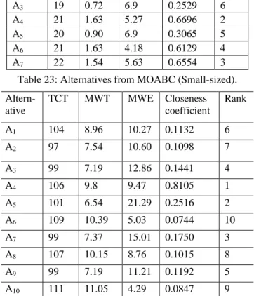
6.3.2.2 Large-size dataset

Table 15 stores the 10 non-dominated solutions emerged

from the large-sized dataset. Each solution is represented with individual job completion time and finally the TCT value of the same sequence, followed by MWT and MWE respectively.

Each best fitted solution for the large-sized dataset is captured as its Pareto front and is represented in figure 18, with its respective fitness values.

The MOABC also yields equally compromising optimized solutions as that of DABC algorithm. The results reveal that the proposed algorithms are superior enough to deal with multi-objectives with a little parameter variation to the canonical ABC. It is a straight forward extension of uni-objective ABC with mixing advantages of local search procedure from the proposed DABC algorithm. We have just applied one of the simplest local search procedure that is two-swap () procedure to optimize the local optima which definitely helps in reducing the algorithmic complexity.

From the result analysis, apart from the completion time, it is seen that most of time the earliness penalty is more than the tardiness penalty. Hence with a required priority level of all the objectives a decision maker can easily go for making a balanced decision for him by applying a suitable MCDM method.

7 Decision making with

chaotic-TOPSIS

After generating successful optimized solution set, we cannot avoid for selecting an appropriate one among these during the decision making process. MCDM is a successful tool for decision making with conflicting P Final job sequence

& completion time

TCT MW

T

MW E

1 J0 J1 J3 J2 21 2.0 4.36

12 14 18 21

2 J3 J1 J2 J0 20 0.9 5.9

9 11 15 20

3 J1 J3 J0 J2 19 0.72 6.9

5 10 15 19

4 J3 J2 J1 J0 21 1.63 5.27

9 14 16 21

5 J1 J3 J2 J0 20 0.90 6.9

5 10 15 20

6 J3 J2 J0 J1 21 1.63 4.18

9 14 19 21

7 J1 J2 J3 J0 22 1.54 5.63

5 13 17 22

Table 14: Non-dominated job sequence.

P Final job sequence & completion time TCT MWT MWE

1 J2 J3 J4 J5 J6 J7 J8 J9 J0 J1 104 8.96 10.27

24 51 62 72 77 83 87 95 98 104

2 J3 J4 J5 J6 J7 J8 J9 J0 J1 J2 97 7.54 10.60

43 54 64 69 75 79 87 90 96 97

3 J4 J5 J6 J7 J8 J9 J0 J1 J2 J3 99 7.19 12.86

36 56 61 67 71 79 82 88 89 99

4 J5 J6 J7 J8 J9 J0 J1 J2 J3 J4 106 9.8 9.47

55 60 66 70 78 81 87 88 98 106

5 J6 J7 J8 J9 J0 J1 J2 J3 J4 J5 101 6.54 21.29

32 39 43 51 57 63 64 80 91 101

6 J0 J1 J5 J3 J4 J2 J6 J7 J8 J9 109 10.39 5.03

43 49 70 80 88 89 93 98 102 109

7 J1 J2 J6 J4 J5 J3 J7 J8 J9 J0 99 7.37 15.01

27 29 50 60 71 81 86 90 97 99

8 J2 J3 J7 J5 J6 J4 J8 J9 J0 J1 107 10.15 8.76

24 51 61 74 79 89 93 100 102 107

9 J4 J5 J9 J7 J8 J6 J0 J1 J2 J3 99 7.19 11.21

36 56 66 71 75 79 82 88 89 99

10 J0 J1 J5 J4 J3 J2 J6 J7 J8 J9 111 11.05 4.29

43 49 70 80 90 91 95 100 104 111

(16)

criterion. Various methods show their respective efficiency in this regard. By a comparative survey we have concluded to decide the final optimal solution here with in our problem using TOPSIS method which really seems to be fit .We have summarized some of the recent TOPSIS applications followed by the discussions of our motivation.

Li et al. [47] presents a new method based on TOPSIS and response surface method (RSM) for MCDM problems with interval number. Similarly Madi et al. [48] provided a detailed comparison of TOPSIS and Fuzzy-TOPSIS in a systematic and stepwise manner. Sotoudeh-Anvari [49] suggested a stochastic multi-objective optimization model for assigning resource and time in order to search the individuals who are trapped in disaster regions. To reduce the heavy computation of the model, two efficient MCDM techniques, i.e. TOPSIS and COPRAS are employed which tackles the ranking problem. Zavadskas et al. [50] reviewed 105 papers which developed, extended, proposed and presented TOPSIS approach for solving DM problems from 2000 to 2015. Recently Wu et al.[51] proposes an improved methodology for handling ships which uses TOPSIS method to make the final decision.

TOPSIS

TOPSIS was developed by Hwang and Yoon [52] in the year of 1981 as an alternative to the elimination and choice translating reality (ELECTRE) method. The basic idea of TOPSIS is quite simple and it has been originated from a displaced ideal point from which the selected solution has shortest distance [53-54]. Further it is refined [52] to the rank based method by assigning specific orders to the available alternatives. The whole concept is based on the two artificial ideal points; that is the ultimate solution is measured by having longest distance from the positive ideal solution (PIS) and the shortest from the negative ideal solution (NIS). Hence a preference order of all alternatives is generated as per their relative closeness to the ideal solutions. As concluded by Kim et al. [55] and our observations, basic TOPSIS advantages are recorded as:

(i) It is an accepted logic that is focused to

rationale of human choice;

(ii) A scalar value justifies both the ideal

alternatives together;

(iii) Simple algorithmic framework and can easily be

coded to the spreadsheet;

(iv) A straightforward performance evaluation of all

alternatives against the defined criteria which can be clearly visualized and represented for two or more dimensions.

The above defined advantages make TOPSIS an omnipresent MCDM technique as compared with rest techniques [52]. In fact it is a utility-based method that evaluates every alternative directly depending on the

available data in the decision matrices and weights [56]. Apart from this, the simulation comparison [57] of TOPSIS method signifies that it has the fewest rank reversals apart from rest methods in the category. Thus, TOPSIS is chosen as the backbone of MCDM.

The preliminary issue with the method is the normalized decision matrix operation, where randomness is achieved while assigning the criterion weights. Hence a narrow gap derived between the performed measures due to the weighted normalized value of the decision matrix. It can be advantageous to substitute this randomness with a suitable chaotic map. Chaos has a very similar property to randomness with better statistical and dynamical characteristic. Such a dynamic mixing is truly appreciated to enhance solutions potentiality by touching every mode in a multi-objective landscape. Hence the use of a well-suit chaotic map in TOPSIS can be definitely helpful to enhance the decision making by generating preferred randomness in criterion weight.

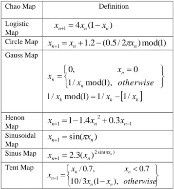
Chaotic maps

Simulation of complex phenomena such as: numerical analysis, decision making, sampling, heuristic optimization etc. needs random sequences for a longer period and good uniformity [58]. Chaotic map is a deterministic, discrete-time dynamic system that is considered as source of randomness, which is non-period, bounded and non-converging [59-60]. However the nature of chaotic maps is apparently random, unpredictable and it has a very sensitive dependence on its initial condition and parameter [58].

A chaotic map can be represented as:

)

12 (

...

3 ,

2 ,

1 ,

0 ,

1 ,

0 ),

(

1

=



=

+

f

x

k

x

_k _k _k

Different selected chaotic maps that produce chaotic numbers in [0, 1] are listed below in table 16 [59-60].