Recursive Algorithms of Closed Loop Identification with a Tailor Made Parameterization

http://www.sciencepublishinggroup.com/j/mlr doi: 10.11648/j.mlr.20170201.13

Recursive Algorithms of Closed Loop Identification with a

Tailor Made Parameterization

Wang Jian-hong

1, 2

1

School of Mechanical and Electronic Engineering, Jingdezhen Ceramic Institute, Jingdezhen, China

2

Dipartimento di Elettronica, Informazione Politecnico di Milano, Milano, Italy

Email address:

[email protected]

To cite this article:

Wang Jian-hong. Recursive Algorithms of Closed Loop Identification with a Tailor Made Parameterization. Machine Learning Research. Vol. 2, No. 1, 2017, pp. 19-25. doi: 10.11648/j.mlr.20170201.13

Received: January 10, 2017; Accepted: February 14, 2017; Published: March 2, 2017

Abstract:

In this paper, we propose two recursive algorithms for closed loop identification under the framework of a tailor made parameterization. The closed loop transfer function is parameterized using the parameters of the open loop plant model, and utilizing knowledge of the feedback controller. When the plant model and feedback controller are all polynomial forms, a recursive least squares method with forgetting schemes is proposed to verify that this recursive method can be regarded as regularization least squares problem. Furthermore we also extend the tailor made parameterization method to nonlinear system and nonlinear controller, then an iterative least squares algorithm is applied to solve one nonlinear optimization problem.

Keywords:

Closed Loop Identification, Tailor Made Parameterization, Recursive Algorithm, Forgetting Schemes

1. Introduction

The whole automatic control system consists of two basic structures-open loop and closed loop structure. As there does not exist any feedback effect between controller and plant model in open loop structure, so the plant output affects the input less. When the effects made by disturbance or external noise may be ignored, the open loop structure is used yet. But now many systems operate under feedback control. This can be due to required safety of operation or to unstable behavior of the plant, as occurs in many industrial production processes like paper production, glass production, separation process like crystallization, etcetera. In closed loop structure, the feedback controller is added to return the collected output back to the collected input. The error signal coming from the input and feedback output can be imposed on the plant to generate one correction action which makes the output converges to one given value. The essences of closed loop structure are to decrease the error using the negative feedback controller, and correct the deviation from the given value automatically. As the closed loop structure can suppress the errors coming from the internal or external disturbances to achieve the control goal, so the closed loop structure is most needed in all of our engineering.

Generally two strategies are used to design the feedback

means that knowledge of the closed loop structure of the configuration, and knowledge of the controller are employed into the parameterization of the closed loop system. One method based on a tailor made parameterization was studied intensively in a linear framework, see [2]. This method applies knowledge of the controller and minimizes an error between the true closed loop transfer function and the model closed loop, using a parameterization model of the open loop model only. In [3], this method was extended to the case of nonlinear systems and nonlinear controllers. The gradient of the identification criterion with respect to the model parameters can be also computed in the nonlinear framework. Further a tailor made instrumental variable parameterization was proposed to identify error-in-variables system, see [4].

Modeling, identification and prediction are three main ubiquitous phenomena in our daily lives. Through our ideas and senses, we collect information about the world, then we interpret, predict and react actions according to our perceptions. In natural science, lots of experiments or observations guide us to formulate laws of nature, which describe different aspects of the world and let us predict all sorts of things, like planet movements or weather forecast. Also in modern technology, modeling and identification have much benefit to offer us one description corresponding to the physical object. Everywhere and everything around us, there is a need for automatic control mechanisms such as in aero-planes, cars, chemical process plants, mobiles phones, heating of houses etc. However to be able to control a system, one needs to know at least something about how it behaviors and reacts to different actions taken on it. Hence we need a model of the system. A system can informally be defined as an entity which interacts with the rest of the world through more or less well defined input and output data. A model is then an approximate description of the system. An ideal model should be simple, accurate and general. This approximate description

of the system can be constructed by system identification strategy, as the goal of system identification is to build a mathematical model of a dynamic system based on some initial information about the system and the measurement data collected from the system. According to [5], the process of system identification consists of designing and conducting the identification experiment in order to collect the measurement data, selecting the structure of the model and specifying the parameters to be identified and eventually fitting the model parameters to the obtained data. Finally the quality of the obtained model is evaluated through model validation process. Generally system identification is an iterative process and if the quality of the obtained model is not satisfactory, some or all of the listed phases can be repeated in order to obtain one satisfied model.

In this note we first study the tailor made parameterization method in a linear framework, where the plant model and controller are all parameterized as polynomials. In order to identify the closed loop parameter vector, a recursive least squares method with forgetting schemes is proposed. This recursive least squares method with forgetting schemes achieves the reformulation of the classical recursive least squares with forgetting schemes as a regularized least squares problem. Secondly we also extend the tailor made parameterization method to nonlinear system and nonlinear controller. During the process of identifying the parameter optimization problem in one nonstandard identification criterion, we use the iterative least squares identification algorithm to generate the iterative sequence.

2. Problem Descriptions

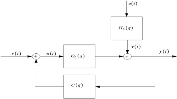
Consider the following closed loop system configuration in Fig. 1.

In Fig. 1 G q0

( )

is a true plant model, H0

( )

q is a noise

filter, they are all linear time invariant transfer functions.

( )

C q is a stable linear time invariant feedback controller, here we assume this controller is priori known. The excited signal r t

( )

and external disturbance e t

( )

are uncorrelated.

( )

e t is a white noise with zero mean value and variance

2

σ

. v t

( )

is a colored noise which can be obtained by passing white noisee t

( )

through that noise filter H0

( )

q .

( )

u t and y t

( )

are the input-output signals with respect to plant model G q0

( )

. qis the time delay operator, it means

that qu t

( ) ( )

=u t+1 .

Observing the closed loop system configuration, we obtain the following transfer function form.

( )

0

( ) ( )

0

( ) ( ) ( )

0

( ) ( )

y t =G q r t −G q C q y t +H q e t (1) Continuing to do some simple computations, we get.

( )

_{( ) ( ) ( )}

( )

_{( ) ( ) ( )}

( )

( )

_{( ) ( ) ( )}

( ) ( )

_{( ) ( ) ( )}

0 0 0 0 0 0 0 1 1 1 1 1

G q H q

y t r t e t

G q C q G q C q C q H q

u t r t e t

G q C q G q C q

 = +  + +    = −  _{+ +}  (2)

To simplify the analysis process, define one sensitivity function as.

( )

_{( ) ( )}

0 0 1 1 S q

G q C q

= +

Applying the defined sensitivity function, the output of closed loop system can be rewritten as.

( )

0

( ) ( ) ( )

0 0

( ) ( ) ( )

0

y t =G q S q r t +H q S q e t

Introduce one unknown parameter vector θ into the closed loop system, the parameterized form corresponding to equation (2) is given as.

( )

_{( ) ( ) ( )}

( )

,

_{( ) ( ) ( )}

( )

,

1 , 1 ,

G q H q

y t r t e t

G q C q G q C q

θ θ

θ θ

= +

+ + (3)

Where θ denotes the unknown parameter vector, it exists in the parameterized plant model G q

( )

,

θ

and noise filter

( )

,

H q

θ

respectively. The goal of closed loop identification is to identify the unknown parameter vector from one given data set

{

( ) ( )

}

1

, N

N

t

Z = r t y t ₌ and priori known controller

( )

C q , where N denotes the total number of observed data [6].

According to equation (3), the prediction of output y t

( )

,

θ

can be calculated as the one step ahead prediction.

( )

( ) ( )

_{( )}

_{( ) ( ) ( )}

( )

( ) ( )

( )

( )

( )

( ) ( )

( )

( )

( ) ( )

( )

1 , ,

ˆ ,

, 1 ,

1 ,

1

,

, , 1 ,

, ,

G q C q G q

y t r t

H q G q C q

G q C q

y t H q

G q H q G q C q

r t y t

H q H q

θ θ

θ

θ θ

θ θ

θ θ θ

θ θ + = × +  ₊  + −      − − = + (4)

We construct one step ahead prediction error or residual as.

( ) ( ) ( ) 1 ( ) ( )_{( )}, ( ) _{( ) ( ) ( )}( ), ˆ

, ,

, 1 ,

G q C q G q

t y t y t y t r t

H q G q C q

θ θ

ε θ θ

θ θ   + = − =  −  +     (5)

In the standard prediction error algorithm [7], using input-output data set

{

( ) ( )

}

1

, N

N

t

Z r t y t

=

= with the number

N, the unknown parameter vector is identified by solving one optimization problem.

(

)

2

( )

1 1

ˆ _{arg min ,} N _{arg min} N _,

N N

t

V Z t

N

θ θ

θ

θ

ε

θ

=

= =

∑

(6)

The above equation (6) is similar to the classical prediction error algorithm and direct approach [8]. In next section it will be made clear that a tailor made parameterization is used. The parameterized plant model G q

( )

,

θ

and feedback controller

( )

C q are all assumed to be polynomials. Then we propose a recursive least squares method with forgetting schemes to identify the unknown parameter vectorθ.

3. Tailor Made Parameterization as

Polynimial Forms

Let the plant model G q

( )

,

θ

be parameterized as one polynomial.

( )

( )

_{( )}

1 1 1 1 , , , 1 b b a a n n n n b q b q B q

G q

A q a q a q θ θ θ − − − − + = = + + ⋯

⋯ (7)

Where _{1 1}

a b

T

n n

a a b b

θ₌_ ⋯ ⋯ _{ . Similarly the} feedback controller is parameterized as.

( )

_{( )}

( )

0 1 1 1 1 1 N N D D n n c n c n

n n q n q N q

C q

D q d q d q

− − − − + + = = + + ⋯

⋯ (8)

Where Nc

( )

q and D qc

( )

are coprime polynomials [9]. Based on these two polynomial forms (7), (8), the parameterization of the output predictor is given by.

(

)

_{( ) ( )}

( ) ( )

,

_{( ) ( ) ( )}

ˆ / 1,

, ,

c

c c

D q B q

y t t r t

D q A q N q B q

θ

θ

θ

θ

− =

The denominator of the closed loop transfer function can be written as a function of the open loop unknown parameter vectorθ.

( ) ( )

( ) ( )

1 2

, , 1 n

c c cl

D q A qθ +N q B qθ = +_q− q− ⋯ q− _θ (10) The order of the closed loop polynomial is given by.

(

)

max _{a D}, _{b N}

n= n +n n +n

The closed loop parameter vector θclis given as.

cl S

θ = θ ρ+ (11)

Matrix Sand vector ρ are parameterized as.

1

0 1

1 0 2 1

2 1

0 1

1 2

0 0 ,

0 0

1 0 0

0 0

1

1 ,

0

0

0 0

D

D

N

N

D

T _{n D N}

n

D N

n

n

n n

P P

d d R S

n d

n n

d d

n n

n

P P

d d

n n

d

n d

ρ₌_ _{ ∈ =}_ _

 

 

 

 

 

 

 

 

 

 

 

 

=_{ } = 

 

 

 

 

 

 

 

  _{ }

 

 

 

⋯ ⋯

⋯

⋯ ⋯ ⋮

⋯ ⋮ ⋱ ⋮

⋯ ⋮ ⋮

⋮ ⋮ ⋯ ⋱

⋯ ⋱

⋮ ⋯ ⋮

⋮ ⋮

⋯ ⋯

(12)

The derivation of equation (12) can be seen [10]. When the feedback controller C q

( )

is priori known, then matrix Sand vector ρ can be constructed by using parameters in coprime polynomials.

Rearranging equation (9), we obtain.

( ) ( )

,

( ) ( ) ( )

,

( ) ( ) ( )

,

c c c

D q A qθ +N q B qθ y t = D q B qθ r t

   

    (13)

Substituting (10), (11) and (12) into (13), it yields.

(

)

(

1 2

)

( )

1 2

[

]

( )

1+_q− q− ⋯ q−n_ P_D P_N θ ρ+ _ y t =_q− q− ⋯ q−n_ 0 P_D θr t (14)

Expanding above equation, we see that.

( )

( ) (

1 2

)

(

) (

_{D N}

)

( ) (

1 2

)

(

)

[

0 _D

]

y t +_y t− y t− ⋯ y t−n  _{ } P P θ ρ+ _=_r t− r t− ⋯ r t−n _ P θ _{It means that.}

( )

(

(

1

) (

2

)

(

)

[

0 _D

]

(

1

) (

2

)

(

) (

_{D N}

)

)

y t = _r t− r t− ⋯ r t−n _ P −_y t− y t− ⋯ y t−n _ P P θ

Defining one vector

ϕ

( )

t as.

( )

(

( ) (

1 2

)

(

)

[

0

]

(

1

) (

2

)

(

) (

)

)

T

D D N

t r t r t r t n P y t y t y t n P P

ϕ = _ − − ⋯ − _ −_ − − ⋯ − _

Then output of the closed loop system can be written as.

( )

T

( )

y t =

ϕ

t

θ

(15)

Vector

ϕ

( )

t is similar to the classical regression vector. A common way to identify the unknown parameter vector θ in (15) relies on the recursive least squares with forgetting schemes, where parameter vector estimation

θ

ˆ_t is given as.

( )

1 ˆ _{arg min}

t V

θ

θ

=

θ

(16)

Where the loss function is defined as.

( )

(

( )

( )

)

1

1

t

t s T

s

V

θ

λ

− y s

ϕ

s

θ

=

=

∑

− (17)

The forgetting factor

λ

∈

[ ]

0,1 operates as an exponential weight which decreases with the more remote data. Optimization problem (16) admits the recursive solution.

( ) ( )

( ) ( )

(

( )

)

1 1

1 1

ˆ ˆ ˆ

T

t t

T

t t t t

R R t t

R t y t t

λ ϕ ϕ

θ θ ϕ ϕ θ

− −

− −

 _{= +}

 

= + −

Define 1

t t

P =R− , then one equivalent recursion is obtained.

( )

( )

(

)

( )

( )

( )

( )

(

)

1 1

1 1

1

ˆ ˆ ˆ

1

T

t t t t

t

t T

t

T

t t t

K y t t

P t

K

t P t

P I K t P

θ θ ϕ θ

ϕ

λ ϕ ϕ

ϕ λ

− −

−

−

−

= + −

= +

= −

(19)

Observing optimization problem (16) again, let

(

₁ t 1

)

t

Q =diag ⋯ λ− _{and consider}

( )

( )

(

)

( )

( )

(

)

(

( )

( )

)

( )

( )

(

)

(

( )

(

)

)

(

( )

( )

)

( )

(

)

2 1

1

2 2 ₁

1

1 2

2 ₁

1 1 1

1

ˆ _{arg min}

arg min

ˆ ˆ ˆ

arg min 2

t

T t i

t

i

t

T T t i

i t

T T T T t i

t t t

i

y i i

y t t y i i

y t t i y i i t

θ

θ

θ

θ ϕ θ λ

ϕ θ λ ϕ θ λ

ϕ θ λ ϕ θ θ ϕ θ ϕ θ θ λ

−

=

−

− −

= −

− −

− − −

=

= −

= − + −

 

= − + _ − − − − _

∑

∑

∑

(20)

Where we use the following relation.

( )

( )

(

)

1

2 ₁ 1

1

ˆ _{arg min}t T t i

t

i

y i i

θ

θ

−

ϕ

θ λ

− −

−

=

=

∑

−

By optimality condition, it holds that.

( )

( )

(

)

2

(

) (

)

1 1 1

ˆ _{arg min} T ˆ T ˆ

t y t t t Rt t

θ

θ = −ϕ θ +λ θ θ− − − θ θ− − (21)

Where the updating law can be seen equation (19). Equation (21) shows that the recursive least squares with forgetting scheme can be regarded as regularization least squares problem.

4. Tailor Made Parameterization as

Nonlinear Systems

In this section we consider the parameterized form (3) again, but we assume the plant model G q

( )

,

θ

and feedback controller C q

( )

are all nonlinear time invariant systems [11], not the polynomials.

Applying the one step ahead prediction error

ε θ

( )

t, , we make use of the identification criterion.

( )

( ) ( )

2

2

1 1

, 2

N

t

V

θ

y t y t

θ

=

=

∑

_ − _ (22)

Where y t

( )

,

θ

is given as

( )

_{( ) ( ) ( )}

( )

_{( ) ( ) ( )}

1 ,

1 1

G

y t r t v t

G C q G C q θ

θ

θ θ

= +

+ + (23)

As to solve the identification criterion V₂

( )

θ with nonlinear plant model G

( )

θ and nonlinear feedback controller C q

( )

, we propose one iterative least squares identification algorithm to generate one iterative sequence. To simplify the latter computation, we define one vector as.

( )

( ) ( ) ( ) ( )

1 1, 2 2,

( ) (

,

)

T

Y θ =_y −y θ y −y θ ⋯ y N −y Nθ _ Then identification criterion V₂

( )

θ can be rewritten as.

( )

( ) ( )

2

1 2

T

V θ = Y θ Y θ

The gradient of y t

( )

,θ with respect to unknown parameter vector θ is that.

( )

( )

(

( ) ( )

)

( )

( )

( ) ( )

( )

( ) ( )

( )

( )

( )

( ) ( )

( )

( ) ( )

( )

( )

2 2

2 2

1 ,

1 1

1 1

G G C q G CG

y t CG

r t v t

G C q G C q

G CG

r t v t

G C q G C q

θ θ θ θ

θ θ

θ _{θ θ}

θ θ

θ θ

′ + − ′ ′

∂

= −

∂ _{ +} _ _{ +} _

′ ′

= −

+ +

   

   

(24)

( )

( )

( ) ( )

( )

( )

( ) ( )

( )

2

2 2

,

1 1

u t CG C G

r t v t

G C q G C q

θ

θ

θ

θ

_θ

_θ

′ ′

∂

= − −

∂ _{ +} _ _{ +} _ (25)

Where we use the following notation.

( )

G t

( )

,

G

θ

θ

θ

∂

′ =

∂

Assume M

( )

θ

is a Jacobian matrix with respect to vectorY

( )

θ

, then M

( )

θ

can be computed as that.

( )

( )

( )

( )

(

)

(

)

(

)

1 2

1 2

1, 1, 1,

, , ,

n

n

y y y

M

y N y N y N

θ θ θ

θ θ θ

θ

θ θ θ

θ θ θ

∂ ∂ ∂

 

 

∂ ∂ ∂

 

 

=_{ }

∂ ∂ ∂

 

 _{∂ ∂ ∂} 

 

⋯

⋮ ⋮ ⋮ ⋮

⋯

(26)

Where the elements of matrix M

( )

θ

can be seen equation (24) and n is the number of unknown parameters. Then the gradient of identification criterion V2

( )

θ

is that.

( )

( ) ( ) ( )

( ) ( ) ( ) ( )

( ) (

)

( )

( )

(

)

( ) ( )

1 1

, ,

2

1, 2,

1 1, 2 2, ,

,

N

t

T

g y t y t y t

y y

y y y y y N y N

y N

Y M

θ θ θ

θ θ

θ θ θ

θ

θ θ

=

′ = _ − _

′

 

 _′ 

 

=_ − − − _{ }



 

′

 

 

=

∑

⋯

⋮

(27)

We continue to compute the Hessian matrix of identification criterionV2

( )

θ

.

( )

(

( ) ( )

( ) ( ) ( )

)

( )

( ) ( )

( )

( ) ( ) ( )

1

1

1

, , , ,

2 1

, ,

2 N

T

t N

t

N y t y t y t y t y t M M S

S y t y t y t

θ θ θ θ θ θ θ θ

θ θ θ

=

=

′ ′ ′′

= +_ − _ = + ′′

= _ − _

∑

∑

(28)

So the quadratic model of identification criterion is that.

( )

( )

( )(

) (

) ( )(

)

( ) ( )

(

( ) ( )

)

(

) (

)

(

( ) ( ) ( )

)

(

)

2

1 2

1 1

2 2

T T

k k k k k k k

T T

T T

k k k k k k k k k k

m V g N

Y Y M Y M M S

θ θ θ θ θ θ θ θ θ θ

θ θ θ θ θ θ θ θ θ θ θ θ θ

= + − + − −

= + − + − + −

(29)

The iterative expression is computed as.

( ) ( ) ( )

(

)

1

( ) ( )

1

T

k k M k M k S k M k Y k

θ + =θ − θ θ + θ − θ θ (30)

Where θ_kdenotes the iterative value at time instantk.

But in iterative expression (28), that quadratic information term S

( )

θ

k can not be computed easily. So we neglect this quadratic information termS

( )

θ

k , and equation (29) is that.

( )

1

( ) ( )

(

( ) ( )

)

(

) (

1

)

(

( ) ( )

)

(

)

2 2

T T

T T

k k k k k k k k k k

Then equation (30) is simplified as.

( ) ( )

(

)

( ) ( )

( ) ( )

(

)

( ) ( )

1 1

1

T

k k k k k k k k

T

k k k k k

M M M Y s

s M M M Y

θ θ θ θ θ θ θ

θ θ θ θ

− +

−

 _{= − = +}

 

 _{= −}



(32)

Generally we summarize the following iterative steps corresponding to the identification criterion at time instantk.

(1)solve

(

MT

( ) ( )

θk M θk

)

sk = −M

( ) ( )

θk Y θk (2)set

1

k k sk θ + =θ +

From the iterative expression (32), we see that this iterative least squares identification algorithm needs only the first derivation information of residual function and matrix

( ) ( )

(

T

)

k k

M θ M θ is positive semi-definite.

5. Conclusion

In this paper we present two kinds of identification algorithms for a closed loop identification scheme with tailor made parameterization. Our main contributions are these: (1) a recursive least squares methods with forgetting schemes is proposed when the plant model and feedback controller are all polynomials. (2) an iterative least squares algorithm is applied to solve one nonlinear optimization problem. Further in future the next subject is about how to extend the tailor made parameterization to dynamic networks with error-in-variables structure.

References

[1] Edwin T, Van Donkellar, “Analysis of closed loop identification with a tailor made parameterization,” European Journal of Control, vol. 6, no. 1, pp. 54-62, 2002.

[2] Franky De Bruyne, “Gradient expressions for a closed loop identification scheme with a tailor made parameterization,”

Automatica, vol. 35, no. 11, pp. 1867-1871, 1999.

[3] Arne Dankers, Paul M J Vandenhof, “Errors-in-variables identification in dynamic networks-consistency results for an instrumental variable approach,” Automatica, vol. 62, no. 12, pp. 39-50, 2015.

[4] Mathieu Pouliquen, Olivier Gehan, “Bounded error identification for closed loop systems,” Automatica, vol. 50, no. 7, pp. 1884-1890, 2014.

[5] Ljung, L, “System identification: Theory for the user,” Prentice Hall, 1999.

[6] Urban Forssel, Lennart Ljung, “Closed loop identification revisted,” Automatica, vol. 35, no. 7, pp. 1215-1241, 1999. [7] Per Hagg, Johan Schoukens, “The transient impulse response

modeling method for non-parametric system identification,”

Automatica, vol. 68, no. 6, pp. 314-328, 2016.

[8] Kaushik Mahata, Johan Schoukens, “Information matrix and D-optimal design with Gaussian inputs for Wiener model identification,” Automatica, vol. 69, no. 7, pp. 65-77, 2016. [9] Hakan Hjalmarsson, Brett Ninness, “Least squares estimation

of a class of frequency functions: a finite sample variance expression,” Automatica, vol. 42, no. 2, pp. 589-600, 2006. [10] G. Pillonetto, “Kernel methods in system identification,

machine learning and function estimation: a survey,”

Automatica., vol. 50, pp. 657–682, Mar. 2013.