Open Peer Review
Any reports and responses or comments on the article can be found at the end of the article.
RESEARCH ARTICLE
Accumulation Bias in meta-analysis: the need to consider
time
in
error control [version 1; peer review: 2 approved]
Judith ter Schure
, Peter Grünwald
Machine Learning, CWI, Science Park 123, 1098 XG Amsterdam, The Netherlands
Abstract
Studies accumulate over time and meta-analyses are mainly retrospective. These two characteristics introduce dependencies between the analysis
, at which a series of studies is up for meta-analysis, and results within time
the series. Dependencies introduce bias — Accumulation Bias — and invalidate the sampling distribution assumed for p-value tests, thus inflating type-I errors. But dependencies are also inevitable, since for science to accumulate efficiently, new research needs to be informed by past results. Here, we investigate various ways in which time influences error control in meta-analysis testing. We introduce an Accumulation Bias Framework that allows us to model a wide variety of practically occurring dependencies including study series accumulation, meta-analysis timing, and approaches to multiple testing in living systematic reviews. The strength of this
framework is that it shows how all dependencies affect p-value-based tests in a similar manner. This leads to two main conclusions. First, Accumulation Bias is inevitable, and even if it can be approximated and accounted for, no valid p-value tests can be constructed. Second, tests based on likelihood ratios withstand Accumulation Bias: they provide bounds on error probabilities that remain valid despite the bias. We leave the reader with a choice between two proposals to consider time in error control: either treat individual (primary) studies and meta-analyses as two separate worlds — each with their own timing — or integrate individual studies in the
meta-analysis world. Taking up likelihood ratios in either approach allows for valid tests that relate well to the accumulating nature of scientific knowledge. Likelihood ratios can be interpreted as betting profits, earned in previous studies and invested in new ones, while the meta-analyst is allowed to cash out at any time and advice against future studies.
Keywords
meta-analysis, accumulation bias, sequential, cumulative, living systematic reviews, likelihood ratio, research waste, evidence-based research
This article is included in the Mathematical,
collection. Physical, and Computational Sciences
Reviewer Status
Invited Reviewers
version 1
25 Jun 2019
1 2
report report
, Columbia University, New York Steven P. Ellis
City, USA 1
, Radboud University Joanna IntHout
Medical Center, Nijmegen, The Netherlands 2
25 Jun 2019, :962 ( First published: 8
)
https://doi.org/10.12688/f1000research.19375.1
25 Jun 2019, :962 ( Latest published: 8
)
https://doi.org/10.12688/f1000research.19375.1
Judith ter Schure ( )
Corresponding author: [email protected]
: Conceptualization, Formal Analysis, Software, Visualization, Writing – Original Draft Preparation, Writing – Review & Author roles: ter Schure J
Editing; Grünwald P: Formal Analysis, Funding Acquisition, Writing – Original Draft Preparation, Writing – Review & Editing No competing interests were disclosed.
Competing interests:
This work is part of the NWO TOP-I research programme Safe Bayesian Inference [617.001.651], which is financed by the Grant information:
Netherlands Organisation for Scientific Research (NWO).
© 2019 ter Schure J and Grünwald P. This is an open access article distributed under the terms of the
Copyright: Creative Commons Attribution
, which permits unrestricted use, distribution, and reproduction in any medium, provided the original work is properly cited.
License
ter Schure J and Grünwald P.
How to cite this article: Accumulation Bias in meta-analysis: the need to consider time in error control
F1000Research 2019, :962 ( )
[version 1; peer review: 2 approved] 8 https://doi.org/10.12688/f1000research.19375.1
25 Jun 2019, :962 ( )
1
Introduction
Meta-analysis refers to the statistical synthesis of results from a series of studies. [...] the synthe-sis will be meaningful only if the studies have been collected systematically. [...] The formulas used in meta-analysis are extensions of formulas used in primary studies, and are used to address similar kinds of questions to those addressed in primary studies. —Borenstein, Hedges, Higgins & Rothstein (2009, pp. xxi-xxiii)
To consult the statistician after an experiment is finished is often merely to ask him to conduct a post mortem examination. He can perhaps say what the experiment died of. —Fisher (1938, p. 18)
These two quotes conflict. Most meta-analyses are retro-spective and consider the number of studies available — after the literature has been searched systematically — as a given for the statistical analysis. P-value based statis-tical tests, however, are intended to be prospective and require the sample size — or the stopping rule that pro-duces the sample — to be set specifically for the planned statistical analysis. The second quote, by the p-value’s pop-ularizer Ronald Fisher, is about primary studies. But this prospective rationale influences meta-analysis as well be-cause it also involves the size of the study series: p-value tests assume that the number of studies — so the timing of the meta-analysis — is predetermined or at least un-related to the study results. So by using p-value meth-ods, conventional meta-analysis implicitly assumes that promising initial results are just as likely to develop into (large) series of studies as their disappointing counter-parts. Conclusive studies should just as likely trigger meta-analyses as inconclusive ones. And so the use of p-value tests suggests that results of earlier studies should be un-known when planning new studies as well as when plan-ning meta-analyses. Such assumptions are unrealistic and actively argued against by theEvidence-Based Research Net-work(Lund et al.,2016) part of the movement to reduce research waste (Chalmers and Glasziou,2009;Chalmers et al.,2014). But ignoring these assumptions invalidates conventional p-value tests and inflates type-I errors. P-values are based on tail areas of a test statistic’s sam-pling distribution under the null hypothesis, and thus re-quire this distribution to be fully specified. In this paper we show that the standard normalZ-distribution generally assumed (e.g. Borenstein et al.(2009)) is not an appro-priate sampling distribution. Moreover, we believe that no sampling distribution can be specified that fully represents the variety of processes in accumulating scientific knowl-edge and all decision made along the way. We need a more flexible approach to testing that controls errors regardless of the process that spurs the meta-analysis.
When dependencies arise between study series size or meta-analysis timing and results within the series, bias is introduced in the estimates. This bias is inherent to ac-cumulating data, which is why we gave it the name Accu-mulation Bias. Various forms of Accumulation Bias have been characterized before, in very general terms as “bias introduced by the order in which studies are conducted” (Whitehead,2002, p. 197) and more specifically, such as bias caused by the dependence of follow-up studies on pre-vious studies’ significance and the dependence of meta-analysis timing on previous study results (Ellis and Stew-art, 2009). Also, more elaborate relations were studied between the existence of follow-up studies, study design and meta-analysis estimates (Kulinskaya et al.,2016). Yet no approach to confront these biases has been proposed. In this paper we defineAccumulation Bias to encompass processes that not only affect parameter estimates but also the shape of the sampling distribution, which is why only approximation and correction for bias does not achieve valid p-value tests. We illustrate this by an example in Sec-tion3, right after we give a general introduction to Accu-mulation Bias in Section2with its relation to publication bias (Section2.1) and an informal characterization of the direction of the bias (Section2.2). By presenting its diver-sity, we argue throughout the paper that any efficient sci-entific process will introduce some form of Accumulation Bias and that the exact process can never be fully known. We collect the various forms of Accumulation Bias into one framework (Section4) and show that all are related to the
timeaspect in meta-analysis. The framework incorporates dependencies mentioned byWhitehead(2002),Ellis and Stewart(2009) andKulinskaya et al.(2016) as well the effect of multiple testing over time in living systematic re-views (Simmonds et al.,2017). We conclude that some version of these biases will also be introduced by Evidence-Based Research.
7.1and7.2, but also give some extra intuition on the magic of likelihood ratios in Section9: Likelihood ratios have an interpretation as betting profit that can be reinvested in future studies. At the same time, the meta-analyst is al-lowed to cash out at any time and advise against future studies. Hence, the likelihood ratio relates the statistics of Accumulation Bias to the accumulating nature of scientific knowledge, which is critical in reducing research waste.
2
Accumulation Bias
Any meta-analyst carries out a meta-analysis under the as-sumption that synthesizing previous studies will add to what is already known from existing studies. So meta-analyses are mainly performed on series of studies of meaningful series size. What is considered meaningful varies considerably: 16 and 15 studies per meta-analysis were reported to be the median numbers inMedline meta-analyses from 2004 and 2014 (Moher et al.,2007a;Page et al.,2016), while 3 studies per meta-analysis were re-ported in Cochrane meta-analyses from 2008 (Cochrane Database of Systematic Reviews(Davey et al.,2011)). Since meta-analyses are performed on research hypotheses that have spurred a certain study series size, they always report estimates that are conditioned on the availability of such a series. The crucial point is that not all pilot studies or small study series will reach a meaningful size, and that doing so might depend on results in the series. Apart from the dependent size of the study series, the exact timing of a meta-analysis can also depend on the available results. The completion of a highly powered or otherwise conclu-sive study, for example, might be considered to finalize the series and trigger a meta-analysis. So meta-analysis also report estimates conditioned on the consideration that a systematic synthesis will be informative. Both dependen-cies — series size and meta-analysis timing — introduce bias: Accumulation Bias.
2.1 Accumulation Bias vs. publication bias
Publication bias refers to the practice that studies with nonsignificant, or more general, unsatisfactory results have smaller probability to be published than studies with significant, satisfactory results. So unsatisfactory studies are performed, but do not reach the meta-analyst because they are stashed away in a file drawer (Rosenthal,1979). Accumulation Bias, on the other hand, refers to some stud-ies or meta-analyses not being performed at all, as a result of previous findings in a series of studies. In a file drawer-free world, Accumulation Bias would still exist. But Ac-cumulation Bias is a manageable problem because it does not operate at the individual study level. Conditional on the fact that a second study is performed, the second study is an unbiased sample. Conditional on the fact that a third study is performed, for whatever reason, the third study is
an unbiased sample. So bias is introduced at the level of the series, not at the study level. This is different for pub-lication bias, where, conditional on being published, the studies available are not an unbiased sample. We exploit the difference in this paper by considering timein error control.
Of course, Accumulation Bias and publication bias are not alone in their effects on meta-analysis reporting. All sorts of significance chasing biases — selective-outcome bias, selective analysis reporting bias and fabrication bias — might be present in the study series up for meta-analysis, and can lead to “wrong and misleading answers” (Ioanni-dis,2010, p. 169). But for a world in which these biases are overcome, we also need tests that reflect how scientific knowledge accumulates.
2.2 Accumulation Bias’ direction
Accumulation Bias in estimates is mainly bias in the satis-factory direction, which means that the effect under study is overestimated. This is the case for bias caused by size of the studies series when (overly) optimistic initial es-timates (either in individual studies or in intermediate meta-analyses) give rise to more studies, while disappoint-ing results terminate a series of studies. This is also the case when the timing of the meta-analysis is based on an (overly) optimistic last study estimate or an (overly) opti-mistic meta-analysis synthesis is considered the final one. We focus on this satisfactory direction of Accumulation Bias and will only briefly discuss other possibilities in Sec-tion5.3and6.1. We introduce the wide variety of possible dependencies in anAccumulation Bias Frameworkin Sec-tion4, which has a generality that also includes Accumu-lation Bias without a clear direction. But we first present Accumulation Bias’ effects on error control by an example.
3
A
Gold Rush
example: new studies
after finding significant results
We study the effect of Accumulation Bias by a simple exam-ple. Its simplicity allows us to calculate the exact amount of bias in the test statistic and investigate the additional effect on the sampling distribution. The example given in this section is an extension of the toy example introduced byEllis and Stewart(2009). We denote this example by
series and the results within: Accumulation Bias. We spec-ify this mechanism in detail in Section3.2and3.3, after we simplified our meta-analysis setting to common/ fixed-effects meta-analysis in Section3.1. We present the result-ing bias in the test estimates in Section3.4and its addi-tional effects on the sampling distribution and testing in Section3.5and3.6. In Section3.7we conclude by point-ing out the very mild condition needed for some form of
Gold RushAccumulation Bias to occur
3.1 Common/fixed-effect meta-analysis
This paper discusses meta-analysis in its simplest form, which is common-effect meta-analysis, also known as fixed-effect meta-analysis. This restriction does not mean that more complex forms of meta-analysis, such as random-effects meta-analysis and meta-regression, do not suffer from the problems mentioned in this paper. The rea-son for simplification is to reduce the complexity in quan-tifying the problem, part of showing that quantification is not enough. In a future paper we will study the effects of heterogeneity on testing in more detail. For an example of Accumulation Bias in random-effects estimates we refer to Kulinskaya et al.(2016).
Common-effect meta-analysis derives a combinedZ-score from the summary statistics of the available studies. This combined Z-score is used as a test statistic in two-sided meta-analysis testing by comparing it to the tails of a stan-dard normal distribution. This is equivalent to assessing whether its absolute value is more thanzα
2 standard
devi-ations away from zero (larger than 1.960 forα= 0.05). We simplify the setting by assuming studies with equal standard deviations to obtain an easy to handle expres-sion for the combined Z-score of t available studies. We denote this meta-analysisZ-score by Z(t)and derive it as the weighted average over the study Z-scores Z1, . . . ,Zt, shown in its general form in Eq. (3.1a) and in Eq. (3.1b) under the assumption of equal study sizes:
Z(t)=
Pt i=1
pn
iZi
p
N(t) with
N(t)=
t
X
i=1
ni (3.1a)
= p1
t
t
X
i=1
Zi (n1=n2=· · ·=nt=n). (3.1b)
See AppendixA.1for a derivation from the mean differ-ence notation inBorenstein et al.(2009).
3.2
Gold Rush
new study probabilitiesIn ourGold Rush example, we assume the following de-pendency within a series of studies: each study in a series has a larger probability to be replicated — and therefore expanding the series of studies — if the study shows a sig-nificant positive effect. So the existence of a new study is
dependent on the significance and sign of the results of its predecessor.
T is the random variable that denotes the maximum size of a study series — the time at which the search stops. We enumerate time by the order of appearance in a study series, with t = 1 for the pilot study, t = 2 for the sec-ond study (so now we have a two-study series) etc. So we use tto denote the number of studies available for meta-analysis at any time point: our notion of time is not re-lated to actual dates at which studies are performed. The maximum time T is usually unknown since more studies might be performed in the future. T ≥2 means that the series has not halted after the first initial study, but that it is unknown how many replications will eventually be per-formed. In our extendedGold Rushexample, we present the Accumulation Bias process by the probability that the maximum size is at least one study larger than the current size (T ≥ t+1), and do so using six parameters. We de-note these parameters by thenew study probabilities, since they indicate the probability that a follow-up study is per-formed when the result of the current study is available:
ω(1) S :=P
T≥2
T≥1,Z1≥zα2
= 1
ω(1) X :=P
T≥2
T≥1,Z1≤ −zα2
= 0
ω(1) NS :=P
T≥2
T≥1,|Z1|<zα2
= 0.1,
for all t≥2 : (3.2)
ω(t)
S = ωS:=P
T ≥t+1
T≥t,Zt≥zα2
= 1
ω(t)
X = ωX:=P
T ≥t+1
T≥t,Zt≤ −zα2
= 0
ω(t)
NS=ωNS:=P
T ≥t+1
T≥t,|Zt|<zα2
= 0.02.
We distinguish between the influence of the first (pilot) study (ω(S1), ω
(1) X andω
(1)
NS) and the others (ωS, ωX and
ωNS) since pilot studies are carried out with future studies in mind, and therefore replications have higher probability after the first than after other studies in the series, also in case the pilot study is not significant. We assume that no new study is performed when a significant negative result is obtained (ω(X1) =ωX =0) and new studies are always performed after positive significant findings, the satisfac-tory result (ω(S1) = ωS = 1). Nonsignificant results have a small, but not negligible probability to spur new studies (ω(NS1)=0.1,ωNS=0.02).
3.3
Gold Rush
new study probabilities’ inde-pendence from data-generating hypothesisIn the following we useP1to express probabilities under
under the null hypothesis. Our new study probabilities in Eq. (3.2) were given without reference to any of these hypotheses, to make explicit that they depend solely on the data (or summary statistic Zt) and not on the hypothesis that generated the data. SoPin these definitions can be read asP1as well asP0.
In the next sections we focus onGold RushAccumulation Bias under the null hypothesis and its effect on type-I error control. The values in rightmost column of Eq. (3.2) are introduced to obtain estimates for the Accumulation Bias in the test estimates. These values are not supposed to be realistic, but are chosen to demonstrate the effect of Accu-mulation Bias as clearly as possible. The extreme values 1 forω(S1) andωS given in Eq. (3.2) support the simula-tion of large study series under the null hypothesis. The small values forω(NS1)andωNSare chosen such that the ef-fect of significant findings on the sampling distribution is clearly visible (see Section3.5and Figure1). Forα=0.05,
ω(1)
S =1 implies that, in expectation under the null distri-bution, all of the 2.5% (α2) positively significant pilot stud-ies under the null hypothesis become a two-study serstud-ies, while ω(NS1) = 0.1 indicates that, since an expected 95% (1−α) of pilot studies is not significant under the null hy-pothesis, 9.5% (0.1·95%) become a two-study series. For study series beyond the pilot study and its replication, this setup entails that in all studies, except for the last and the first, the fraction of significant findings is more than half, sinceωS=0.02 implies that only 0.02·95%=1.9% non-significant studies grow into a larger study series: the ex-pected fraction of significant studies in growing series un-der the null hypothesis converges to 2.5/(2.5+1.9) =0.6.
3.4
Gold Rush
Accumulation Bias’ estimates under the null hypothesisThe new study probability parameters in Eq. (3.2) are much larger when results are positively significant than when they are not. As a result, study series that contain more significant studies have larger probabilities to come into existence than those that contain less. While the ex-pectation of a Z-score is 0 under the null hypothesis for each individual study (for allt:E0[Zt] =0), the expecta-tion of a study that is part of a series of studies is larger. This shift in expectation introduces the Accumulation Bias in the estimates.
The main ingredient of the bias in the meta-analysisZ(t) -score is the bias in the individual study Zt-scores, condi-tional on being part of a series. This is already apparent for the pilot study, which we use as an example by expressing its expected value under the null hypothesis, given that it has a successor study:E0[Z1|T≥2]. This conditional
ex-pectation is a weighted average of two other exex-pectations that are conditioned further based on the events that lead to a new study according to Eq. (3.2): E0Z1
Z1≥zα2
,
Z1 from the right tail of the null distribution, and the nonsignificant results with expectationE0
Z1
|Z1|<zα2
. We discard negative significant results, since those were given 0 probability to produce replication studies in Eq. (3.2). The positive significant and nonsignificant results are weighted by the new study probabilities in Eq. (3.2) and the probabilities under the null distribution of sam-pling from either the tail (α) or the middle part (1−α) of the standard normal distribution. A more detailed specifi-cation of these components can be found in AppendixA.2. If we assume a significance threshold of 5% we obtain:
Forα=0.05 : E0[Z1|T≥2]
=
R∞
zα 2
z·φ(z)dz·ω(1) S ·
α
2+0·ω
(1)
NS·(1−α)
ω(1) S ·α2+ω
(1)
NS ·(1−α)
≈0.487.
(3.3)
Here we use the fact that, forα=0.05,E0Z1
Z1≥zα2
=
R∞
1.960z·φ(z)dz ≈ 2.338, withφ()the standard normal
density function and thatE0Z1
|Z1|<zα2
is the expec-tation of a symmetrically truncated standard normal dis-tribution, which is 0. The value 0.487 is obtained by using the parameter values given in Eq. (3.2). For studies in the series later than the pilot study, the expression follows analogously by taking for allt≥2 :ω(St)=ωSandω
(t) NS =
ωNS:E0[Zt|T≥t+1]≈1.328.
To determine the effect on the meta-analysis Z(t)-score, we define the expectation under the null hypothesis
E0
Z(t)T≥t
, conditioned on the availability of a series of size t. To specify this expectation, we use that the last study is always unbiased since we do not know whether it will spur more studies. As shown in more detail in Ap-pendixA.3, the expression follows from Eq. (3.1a) by sep-arately treating the unbiased expectation of 0 and the pilot study. If we assume a significance threshold of 5%, we ob-tain the general expression in Eq. (3.4a) and the expres-sion in Eq. (3.4b) under the assumption of equal study sizes (n1=n2=· · ·=nt=n):
Forα=0.05, for allt≥2 :
E0Z(t)T≥t
≈ pn
1·0.487+
Pt−1
i=2
pn
i·1.328+pnt·0
p
N(t) (3.4a)
=0.487+1.328p (t−2)
t . (3.4b)
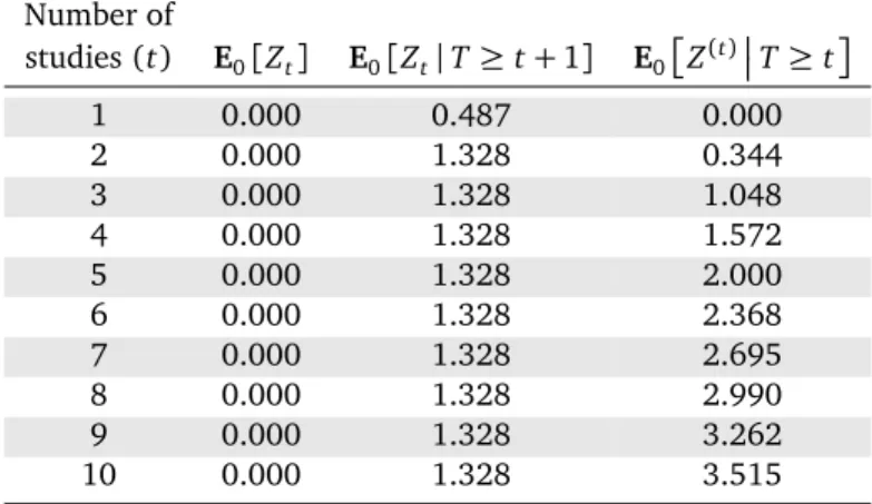
Table1shows the Accumulation Bias in the estimates of E0Z(t)
T≥t
as studies accumulate under theGold Rush
Table 1. Expected Z-scores under the null hypothesis in theGold Rush scenario, under the equal study size
assumption, calculated using Eq.(3.4b)withα=0.05and values forω(S1),ω
(1)
NS,ωSandωNSfrom Eq.(3.2). Z(
t)is
as defined in Eq.(3.1b). See AppendixA.7for the code that was used to calculate these values.
Number of
studies (t) E0[Zt] E0[Zt|T≥t+1] E0
Z(t)T ≥t
1 0.000 0.487 0.000
2 0.000 1.328 0.344
3 0.000 1.328 1.048
4 0.000 1.328 1.572
5 0.000 1.328 2.000
6 0.000 1.328 2.368
7 0.000 1.328 2.695
8 0.000 1.328 2.990
9 0.000 1.328 3.262
10 0.000 1.328 3.515
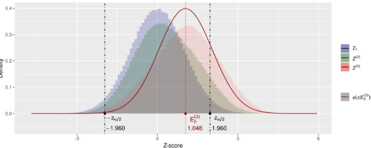
3.5
Gold Rush
Accumulation Bias’ sampling distribution under the null hypothesisFigure1shows simulatedGold Rushsampling distributions for study series of size two and three in comparison to an individual study Z-distribution. Because the new study probabilities in Eq. (3.2) giveZt−1-values below−zα2 zero
probability to warrant a successor study, values for the
z(t)-statistic below −zα
2 will be scarce and the largert is
the larger this scarcity will be since only the last study is able to provide such small Z-score estimates. The oppo-site is the case for values abovezα
2, which have probability
1 to warrant a new study. As a result, the distribution of the meta-analysis Z-score has negative skew (more mass on the right, more tail to the left). See the comparison to the normal distribution also plotted in Figure1 for a three-study series. Skewness is not the only characteristic that distinguishes the resulting distribution from a stan-dard normal. The variance also deviates since the meta-analysis distribution is a mixture distribution.
For a two-study meta-analysis Z(2) we obtain a mixture of two conditional distributions, one conditioned on the first study being a significant — sampled from the right tail of the distribution (with probability α2·ω(S1)) — and one with the first study nonsignificant — sampled from the symmetrically truncated normal distribution (with proba-bility(1−α)·ω(1)
NS). Because the combined distribution on
Z(2)is a mixture of the two scenarios, its variance is larger than the variance of either of the two components of the mixture, as we show in AppendixA.4. In Figure1we see that, with the parameter values from Eq. (3.2) the vari-ance ofZ(2)andZ(3)are even larger than that ofZ1, even though bothVar¦Z(2)
Z1<zα2
©
andVar¦Z(2)
|Z1| ≥zα2
©
are smaller. Hence the sampling distribution under the null hypothesis of a meta-analysisZ-score deviates from a standard normal under Accumulation Bias due to a
non-zero location (the bias), skewness and inflated variance. All three inflate the probability of a type-I error in a stan-dard normal test, as we will study in the next section.
3.6
Gold Rush
Accumulation Bias’ influence on p-value testsLet us now establish the effect of our Gold Rush Ac-cumulation Bias on meta-analysis testing when using common/fixed-effects Z-tests. Let ETYPE(t) -I indicate the
event of a type-I error (significant result under the null hypothesis) in a meta-analysis of t studies and let P0
ETYPE(t) -I
T≥t
=P0
|Z(t)| ≥zα 2
T≥t
denote the ex-pected rate of type-I errors in a two-sided common/ fixed-effect Z-test for studies i up to t conditional on the fact that at leasttstudies were performed.
We obtain the type-I error rate for this test by simulating theGold Rushscenario, for which the results are shown in the right hand column of Table2, assumingα=0.05. If only bias would be at play, the sampling distribution under the null hypothesis would be a shifted normal distribution. Eq. (3.5) expresses the expected type-I error rate for this bias only scenario, withΦ()the cumulative normal distri-bution. The inflation actual inflation in the type-I error rate is larger than shown by this scenario, as illustrated the Table2. The difference between these two type-I error rates for a series of three studies is depicted in Figure 1 by the area under the red histogram for Z(3)and the red
φ(z|E0(3))curve below−zα
2 and abovezα2. We conclude
that the effect of Accumulation Bias on testing cannot be corrected by only an approximation of the bias.
f
P0ETYPE(t) -I
T≥t
:=1−Φzα 2 −E0
Z(t)T ≥t
+Φ−zα 2 −E0
Z(t)T≥t
Figure 1. Sampling distributions of meta-analysisZ(t)-scores under the null hypothesis in theGold Rushscenario,
under the equal study size assumption, withα=0.05and values forω(S1),ω
(1)
NS,ωSandωNSfrom Eq. (3.2). Z(
t)is
as defined in Eq.(3.1b).φ(z|E0(3))the standard normal density function shifted by E
0(3), with E0(3)shorthand for
E0
Z(3) T ≥3
. See AppendixA.7for the code that produces the simulation and this figure.
Table 2. Inflated type-I error rates for tests affected by bias only and tests affected by bias as well as impaired
sampling distribution. Simulated values are under the null hypothesis in theGold Rushscenario, under the equal
study size assumption, withα=0.05and values forω(S1),ωNS(1),ωSandωNSfrom Eq. (3.2). See AppendixA.7for
the code that produces the simulation and this table.
Number of studies (t) fP0[ETYPE(t) -I|T≥t] P0[ETYPE(t) -I|T≥t]
2 0.06 0.10
3 0.18 0.23
4 0.35 0.40
5 0.52 0.53
3.7
Gold Rush
Accumulation Bias: When does it occur?We indicated in Section 3.3 that we chose extreme val-ues for parametersω(S1),ω
(1) X ,ω
(1)
NS,ωS,ωX andωNSsuch that Figure 1 would clearly show the bias and distribu-tional change that occurs. However, for any combination of values for which there is at whereω(St)6=ω
(t) X 6=ω
(t) NS Accumulation Bias occurs for series larger than sizetand p-value tests that assume a standard normal distribution are invalid.
4
The Accumulation Bias Framework
In general, Accumulation Bias in meta-analysis makes the sampling distribution of the meta-analysisZ-score difficult to characterize due to the data dependent size and tim-ing of a study series up for meta-analysis. In this section, we specify both processes in a framework of analysis time probabilities. We use the termanalysis timebecause time
in meta-analysis is partly based on asurvival time. A sur-vival time indicates that a subject lives longer than time
t(and might still become much older), just as an analysis time indicates that a series up for meta-analysis has at least sizet(but might still grow much larger). As such, analy-sis time probabilities, just as the probabilities in a survival function, do not add up to 1.
OurAccumulation Bias Frameworkuses the following nota-tion for its three key components:S(t−1),A(t)andA(t). Firstly,S(t−1)can be understood as the survival function in the variable timetthat indicates the size of the expand-ing study series. S(t−1)denotes the probability that the available number of studies is at leastt(P[T≥t]), so the study series has survived past the previous study att−1. Secondly,A(t)indicates the event that a meta-analysis is performed on a study series of size exactlyt. Lastly,A(t)
prob-ability A(t)represents the general probability that a meta-analysis of sizet— so attime t— is performed and is the key to describing the influence of various forms of Accu-mulation Bias on testing.
4.1 Analysis time probabilities
LetPA(t)T≥t,z1, . . . ,zt
denote the probability that a meta-analysis is performed on the first t studies. Just as theGold Rush’ new study probabilities from Eq. (3.2), this probability can depend on the results in the study series
z1, . . . ,zt. The eventA(t)only occurs if a series of size t is available, so we need to condition on the survival past
t−1, which can also depend on previous results. When combined, we obtain the following definition1ofanalysis
time probabilities A(t):
A(t|z1, . . . ,zt):=PA(t)T≥t,z1, . . . ,zt
·S(t−1|z1, . . . ,zt−1),
where we define
S(t−1|z1, . . . ,zt−1):=P[T ≥t|z1, . . . ,zt−1].
(4.1)
Eq. (4.1) formalizes the idea of analysis time probabilities “depending on previous results” in terms of the individual study Z-scores z1, . . . ,zt. This is compatible with the Z -test approach in meta-analysis and the dependencies and theGold Rush’ new study probabilities that are explicitly expressed in terms of Z-scores. More generally however, in Section4.3and4.4we extend the definition and allow analysis time probabilities to also depend on the data in the original scale and external parameters.
4.2 Analysis time probabilities’ independence
from the data-generating hypothesis
Just as for theGold Rush’ new study probabilities discussed in Section3.2and3.3, the analysis time probabilitiesA(t)
only depend on the data, and are independent from the hypothesis that generated the data. So again,P in these definitions can be read as P1 as well as P0. Our
defini-tion ofA(t)relates to the definition of aStopping Ruleby Berger and Berry(1988, pp. 33-34), where they usex(m)
to denote a vector ofmobservations: 1Note thatA(t
|z1, . . . ,zt)is defined as a product of two (conditional) probabilities. Calling this product itself a “probability”, as we do, can be justified as follows: we currently think of the decision whether to continue studies at timet, i.e. whetherT ≥t, to be made before the t-th study is performed. But we may also think of thet-study resultzt as being generated irrespective of whetherT≥t, but remaining unob-served for ever ifT<t. If the decision whetherT≥tis made indepen-dently of the valuezt, i.e. we add the constraintP[T≥t|z1, . . . ,zt−1] = P[T≥t|z1, . . . ,zt], then the resulting model is mathematically equiva-lent to ours (in the sense that we obtain exactly the same expressions for S(t),A(t|z1, . . . ,zt), all error probabilities etc.), but it does allow us to write, by Eq. (4.1), thatA(t|z1, . . . ,zt) =P
A(t),T≥t z1, . . . ,zt
— so nowA(t|z1, . . . ,zt)is indeed a probability.
Definition. A stopping rule is a sequenceτ =
(τ0,τ1, . . .)in whichτ0∈[0, 1]is a constant and τm is a measurable function of x(m) form≥1, taking values in[0, 1].
τ0is the probability of stopping the experiment
with no observations (e.g., if it is determined that the experiment is too expensive);τ1(x(1))is the probability of stopping after observing the datum
x(1) = x1, conditional on having taken the first observation; τ2(x(2))is the probability of
stop-ping after observing x(2)= (x1,x2), conditional on having taken the first and second observa-tions; etc.
To take the analogy with survival analysis further, we con-sider the sequence τdefined above byBerger and Berry (1988) to be a sequence of hazards. Instead of using their notation τ we denote the Stopping Rule by λ = (λ(0),λ(1), . . .)to emphasize its behavior as a sequence of
hazard functionsand to distinguish timetfrom the proba-bilityλ(t)of stopping at that time given that you were able to reach it. The hazard of stopping at time tcan depend on previous results and is defined as follows:
λ(t|z1, . . . ,zt):=P[T =t|T≥t,z1, . . . ,zt]. (4.2) In this paper we are only interested in cases in which a first study is available, soλ(0) =0 (also stated asP[T ≥1] =1 in AppendixA.2). The survivalS(t−1), the probability of obtaining a series of size at least t (so larger thant−1), follows from the hazards by considering that surviving past timet−1 means that the series has not stopped at studies
iup to and includingt−1. So fort≥1:
S(t−1|z1, . . . ,zt−1) =
t−1
Y
i=0
(1−λ(i|z1, . . . ,zi)). (4.3)
In many examples, the hazard of stopping at time t,λ(t), will depend on the result zt just obtained. In that case
λ(i|z1, . . . ,zi) =λ(i|zi)in Eq. (4.3) above. But in gen-eralλ(t)might also depend on some synthesis of allziso far. We show some of the variety of forms thatλ(t),S(t)
andA(t)can take in our Accumulation Bias Framework in the following sections.
4.3 Accumulation Bias caused by dependent
study series size
4.3.1 Gold Rush: dependence on significant study results
TheGold Rushscenario operates in a general meta-analysis setting and assumes that there is a single random or pre-specified time t at which a study series is up for meta-analysis. This is the approach taken by meta-analyses not explicitly part of a living systematic review. In theGold Rushexample the dependency arises in the study series be-cause at-study series has a larger probability to come into existence when individual study results are significant, and you need at-study series to perform at-study meta-analysis. This dependency was characterized by the new study probabilitiesω(S1),ω
(1)
NS,ωS andωNSfrom Eq. (3.2). The value of S(t), and thereforeA(t), can be expressed in terms of these new study probabilities by considering whetherz1, . . . ,zt−1are larger thanzα
2 (which is 1.960 for α=0.05). Since a meta-analysis is performed only once at a randomly chosen timet, we haveP[A(t)] =1 for that time tandP[A(t)] =0 otherwise. So for the one meta-analysis we obtain:
Fortsuch that P[A(t)] =1 :
A(t|z1, . . . ,zt−1;α) =S(t−1|z1, . . . ,zt−1;α)
= t−1
Y
i=0
(1−λ(i|zi;α)),
(4.4)
withλ(0) =0 and for alli≥1,λ(i)is defined as follows:
λ(i|zi,α) =1−
ω(i)
S ·1zi≥zα2 +ω
(i)
NS·1|zi|<zα2
λ0(i|α):= E0[λ(i|Zi;α)] =1−ω(i)S ·
α
2 +ω (i)
NS·(1−α)
.
(4.5)
Therefore, (leaving out theλ(0)and summing fromi=1 tot−1), we obtain the following expressions for theGold Rushanalysis time probabilities and its expectations under the null distribution:
A(t|z1, . . . ,zt−1;α) =
t−1
Y
i=1
ω(i)
S ·1zi≥zα2 +ω
(i)
NS·1|zi|<zα2
A0(t|α):=E0[A(t|Z1, . . . ,Zt−1;α)]
= t−1
Y
i=1
ω(i)
S ·
α
2+ω (i)
NS·(1−α)
.
(4.6)
4.3.2 Kulinskaya et al. (2016): dependence on meta-analysis estimates
Kulinskaya et al.(2016) report biases that result from de-pendencies between a current meta-analysis estimate and
the decision to perform a new study. Since their focus is on bias, they do not discuss issues of multiple testing over time, which would arise if their cumulative meta-analyses estimates were tested. In this section we assume that the timing of the meta-analysis test is independent from the estimates that determined the size of the series, as if a test were done by a second unknowing meta-analyst. This sce-nario is hinted at byKulinskaya et al.(2016, p. 296) in the statement “When a practitioner or a meta-analyst finds several trials in the literature, a particular decision-making scenario may have already taken place.” We postpone the discussion of multiple testing to Section4.3.4. In this es-timation setting, the decision to perform new studies is determined not by the meta-analysisZ-scores Z(t−1), but by the meta-analysis estimates on the original scaleM(t−1) (notation adopted fromBorenstein et al.(2009), see Ap-pendixA.1), in relation to a minimally clinically relevant effect ∆H1. A minimally clinically relevant effect is the
effect that should be used to power a trial (in the alter-native distribution H1), and therefore, the effect that the researchers of the study do not want to miss. Kulinskaya et al.(2016) consider three models for the study series ac-cumulation process: thepower-law modeland the extreme-value modeland theprobit model. The models relate the probability of a new study to the cumulative meta-analysis estimate of the study series so far and are inspired by mod-els for publication bias. Although all three modmod-els can be recast in our framework, we demonstrate this only for the power law model that uses one extra parameterτto re-late the previous meta-analysis estimate M(t−1) to S(t). Just as in theGold Rushscenario, we must assume that a meta-analysis test is performed only once at a randomly chosen time t. So only at that time t P[A(t)] = 1 and P[A(t)] = 0 otherwise. We obtain the following expres-sion for theKulinskaya et al.(2016)power-law model:
Fortsuch that P[A(t)] =1 :
A tM(t−1);∆H1,τ
=S t−1M(t−1);∆H1,τ
= t−1
Y
i=0
(1−λ iM(t−1);∆H1,τ
),
(4.7)
withλ(0) =λ(1) =0, and for alli≥2,λ(i)is defined as follows:
λ iM(i−1);∆H1,τ
=1−
M(i−1)
∆H1
τ
, (4.8)
for 0<M(i−1)<∆H1and 1 (so 1−λ=0) otherwise. According to this model, no further studies are performed as soon as an estimate as large as∆H1is found. For
esti-mates smaller than∆H1, the closer the estimate is to∆H1,
as well as skew the sampling distribution of the data un-der the null hypothesis since initial studies with large es-timates have larger probability to end up in study series of considerable size than small initial estimates do. When the initial study gives a large overestimation of the effect, this overestimation stays present in the subsequent meta-analysis estimates and keeps influencing the probability of subsequent studies. Therefore, this model shows the ef-fect of early studies in the series even more clearly than theGold Rushexample. However, the accumulation bias does have a cap, since estimates larger than∆H1 do not
introduce new replication studies.
4.3.3 Whitehead(2002): dependence on early study re-sults
Bias may also be introduced by the order in which studies are conducted. For example, large-scale clinical trials for a new treatment are often undertaken following promising results from small trials.[...]given that a meta-analysis is being undertaken, larger estimates of treat-ment difference are more likely from the small early studies than from the later larger studies. —Whitehead (2002, p. 197)
Whitehead (2002) mentions a dependence between the results of the small early studies in a series and the size of the series. This influence could either be based on the significance of early findings, such as in theGold Rush ex-ample (Section 4.3.1), or on the estimates in the initial studies, such as in the power law model fromKulinskaya et al.(2016) (Section4.3.2).Whitehead(2002) does not give sufficient details to specify this dependency explicitly, but we are confident that it will fit in our Accumulation Bias framework.
Two ways to approach this Accumulation Bias are given in Whitehead(2002). The first is to exclude early stud-ies from the meta-analyses, either in the main analysis or in a sensitivity analysis. The second way is to ignore the problem, since the small studies will have little effect on the overall estimate. In Section7we show that any small initial study dependency that can be expressed in terms of
A(t)can be dealt with by tests using likelihood ratios.
4.3.4 Living Systematic Reviews: dependence on signif-icant meta-analyses + multiple testing
A living systematic review (LSR) should keep the review current as new research evidence emerges. Any meta-analyses included in the re-view will also need updating as new material is identified. If the aim of the review is solely to present the best current evidence standard meta-analysis may be sufficient, provided reviewers are aware that results may change at later up-dates. If the review is used in a decision-making
context, more caution may be needed. When us-ing standard meta-analysis methods, the chance of incorrectly concluding that any updated meta-analysis is statistically significant when there is no effect (the type I error) increases rapidly as more updates are performed. —Simmonds, Salanti, McKenzie & Elliott (2017, p. 39)
In living systematic reviews, the aim is to have a meta-analysis available to present the current evidence, thus synthesizing thetstudies available at a certain time. The current meta-analysis estimate might be used to decide whether further studies should be performed. In that case
S(t−1), the probability that a study series of sizetis avail-able — so that a study series has expanded beyond series sizet−1 — depends on the meta-analysis estimateZ(t−1)
at the previous study’s meta-analysis. Because the review is continuously updated,P[A]is always 1, and living sys-tematic reviews can be described by the following analysis time probabilityA(t):
At
z
(1), . . . ,z(t);zα
2
=PA(t) T≥t
·St−1
z
(1), . . . ,z(t);zα
2
=St−1
z
(1), . . . ,z(t−1);zα
2
= t−1
Y
i=0
(1−λi
z
(i);zα
2
).
(4.9)
The quote above warns against decisions based on the con-tinuously updated meta-analysis using a fixed threshold
zα
2. Living systematic reviews experience multiple testing
problems of a kind that are familiar from statistical moni-toring of individual clinical trials (Proschan et al.,2006). If the study series is stopped as soon as a significance thresh-old is reached, and the obtained meta-analysis is consid-ered the final one, then this final meta-analysis test has an increased chance of a type-I error. So the warning is not to use the following simple stopping rule:
λ
i
z
(i);zα
2
=1|Z(i)|≥zα 2
. (4.10)
Various corrections to significance thresholds are proposed that relate intermediate looks to a maximum sample size or information size. These corrected thresholds depend on
between “the best current evidence” and the accumulation of future studies is part of our Accumulation Bias Frame-work. We discuss the approach to error control taken by the corrected thresholds in Section5.2.
4.4 Accumulation Bias caused by dependent
meta-analysis timing
We described various forms of Accumulation Bias that are caused by how the study series size comes about, but de-pendencies are also introduced by how the meta-analysis itself arises. This is expressed by thePA(t)
component of the analysis times probabilitiesA(t). We only found one such process mentioned in the literature and will discuss it in the next section.
4.4.1 Ellis and Stewart(2009): dependence on the right amount of positive findings
Meta-analysis times are subtle. A train of neg-ative findings would generally not stimulate a meta-analysis. Nor would a string of very pos-itive findings. [...] All this makes the analysis of explicitly defined meta-analysis times very dif-ficult. We conclude that study of bias in analysis based on parametric modeling of meta-analysis times is problematical. —Ellis & Stewart (2009, pp. 2454-2455)
Ellis and Stewart(2009) do not give an explicit model that we can interpret in terms ofA(t), but indicate that it should depend on the study findingsZi, or in the original scale,Di (notation adapted fromBorenstein et al.(2009), see Ap-pendixA.1). Given the quote above, the amount of very positive findings should not be too large, and not too small. Though exact parametric modeling indeed stays problem-atical, we can assume that a positive finding is a study es-timate larger than the minimally clinically relevant effect ∆H1, define the right amount of positive findings to be in
the region[a, b], and show that this fits in our Accumu-lation Bias Framework by expressing a possible model for
A(t):
Fortsuch thatS(t−1) =1 :
A tD1, . . . ,Dt;a,b
=PA(t)T≥t,D1, . . . ,Dt;a,b
·S t−1D1, . . . ,Dt−1;a,b
=P A(t)
T≥t,D1, . . . ,Dt;a,b
=1C∈[a,b]
with C=
t
X
i=1
1Di>∆H1.
(4.11)
4.5 Accumulation Bias caused by
Evidence-Based Research
New research should not be done unless, at the time it is initiated, the questions it pro-poses to address cannot be answered satisfac-torily with existing evidence. —Chalmers & Glasziou (2009)
In 2009, the termResearch Wastewas coined and this key recommendation was made. The recommendation further specifies that existing evidence should be obtained by a systematic review and summarized with a meta-analysis. But how exactly to answer the question whether new re-search is necessary or wasteful remained unclear. Never-theless, the recommendation was important enough to be repeated, as was first done in an entire series on Research Waste with a specific recommendation on setting research priorities (Chalmers et al.,2014) and later in a paper that gave the recommendation its official name:Evidence-Based Research(Lund et al., 2016). Support for these recom-mendations was provided by various retrospective cumu-lative meta-analyses that show how many studies were still performed while satisfactory evidence was already avail-able. These cumulative meta-analysis judge “satisfactory evidence” based on a significance threshold, usually uncor-rected for multiple testing (e.g. Fergusson et al.(2005)), which reminds us of the Accumulation Bias that occurs in living systematic reviews (Section4.3.4).
The larger consequence, however, is that Accumulation Bias is caused by any dependencies between results and series size and meta-analysis timing, and that Evidence-Based Research introduces such dependencies. Inspecting previous results to decide whether new research is neces-sary or wasteful therefore always introduces Accumulation Bias, whether it based on uncorrected or corrected thresh-olds. Also more subtle decision methods — implicit rather than based on thresholds — introduce Accumulation Bias, as was shown byKulinskaya et al.(2016). In fact, they de-scribe the rationale behind their models — among which thepower-lawmodel (Section4.3.2) — as an example of bias introduced by guidelines to decide on “the usefulness of a new study” “with direct reference to existing meta-analysis.” (Kulinskaya et al.,2016, p. 297).
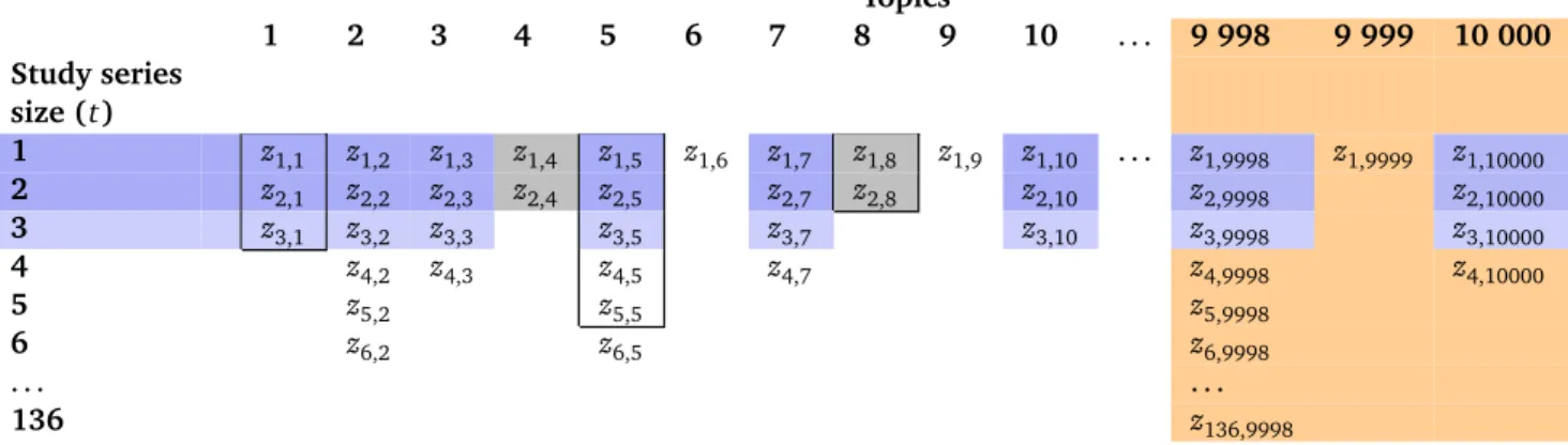
Table 3. Possible 2001 state of a database of study series per topic, visualizing what study series are taken into account in the two approaches to error control: conditional on time (blue and grey) and surviving over time (orange).
Topics
1 2 3 4 5 6 7 8 9 10 . . . 9 998 9 999 10 000
Study series
size (t)
1 z1,1 z1,2 z1,3 z1,4 z1,5 z1,6 z1,7 z1,8 z1,9 z1,10 . . . z1,9998 z1,9999 z1,10000
2 z2,1 z2,2 z2,3 z2,4 z2,5 z2,7 z2,8 z2,10 z2,9998 z2,10000
3 z3,1 z3,2 z3,3 z3,5 z3,7 z3,10 z3,9998 z3,10000
4 z4,2 z4,3 z4,5 z4,7 z4,9998 z4,10000
5 z5,2 z5,5 z5,9998
6 z6,2 z6,5 z6,9998
. . . .
136 z136,9998
5
Time
in error control
Over time new study series are initiated, studies are added to existing study series and more meta-analyses are per-formed. To visualize how this process relates to error con-trol, we need to start with a specific state of this expanding system. In 2001 an estimated minimum of 10 000 medi-cal topics were covered in over half a million studies, thus requiring 10 000 meta-analyses if all were synthesized in a database such as theCochrane Database of Systematic Re-views(Mallett and Clarke,2003). The number of studies in a series varied between 2 and 136, which we can use to describe the 2001 state of a possible database, that to be complete, also includes many unreplicated pilot studies. We could visualize this database in a table, with studies in the rows, topics in the columns and many missing entries. A sketch is shown in Table3.
The conventional approach to error control, which we used to show the influence ofGold RushAccumulation Bias in meta-analysis testing in Section3.6, is a conditional ap-proach. Since conventional meta-analysis does not raise any multiple testing issues, there is a hidden assumption that the timing of a meta-analysis A(t) is independent from the data and each study series experiences only one meta-analysis. In Section 4.3.1 we took the t at which the sole meta-analysis is conducted to be either random or prespecified. This is shown in Table3by the black box enclosing the available studies on Topic 1. Other possible study series up for meta-analysis are shown by the boxes enclosing studies on Topic 5 and 8. Note that by assum-ing only one meta-analysis, a study series might continue growing but not be fully analyzed, as shown for Topic 5. In the conditional approach to error control, a three-study series(Z1,Z2,Z3)produces a possible draw from theZ(3)
sampling distribution. If we test our draw, the type-I error rate is defined as the fraction oft-study series that is con-sidered significant if allt-study series were to be sampled from the null distribution. The question is: What study
series are taken into account to specify this fraction? This is visualized in Table3by the dark blue and grey shading fort =2 and the dark blue and lighter blue shading for
t=3. The unshaded topics and change of color between
t = 2 and t = 3 show the flaw of this approach: some series might not survive up until a specific time t, as for instance shown by the grey studies that are part oft=2 but not part of the error control fort=3. We also do not want every series to survive up until any arbitrary timet
to avoid research waste (Chalmers and Glasziou,2009). The crucial point is that the series that do survive are no random sample from all possible t-study series. This is another illustration of Accumulation Bias such as theToy Storyscenario. The series deviates even more from the as-sumption of a random t-study draw if the meta-analysis time t is not random or prespecified, but dependent on the results, as expressed in Section4.4. We discuss the conventional conditional approach to meta-analysis error control in more detail in Section5.1.
The other possible approach to error control is surviving over analysis times, which means that it should be valid for any upcoming analysis timet within a series. So the probability that a type-I error — ever — occurs in the ac-cumulating series is controlled, whether the series reaches a large size or not. This is visualized in Table3by the or-ange shading, and has a long run error rate that runs over series of any size, including the one-study series. This ap-proach to error control is taken by methods for living sys-tematic reviews such as Trial sequential analysis and Se-quential meta-analysis. We discuss this approach of error control surviving over time in more detail in Section5.2.
5.1 Error control conditioned on time
The null distributions of the common/fixed meta-analysis
description, where we use f0(z(t))to denote the assumed standard normal null distribution for the meta-analysisZ -score and obtain a conditional density using Bayes’ rule:
f0 z(t)A(t),T≥t
= f0(z (t))·P
0
A(t),T≥tz(t)
P0[A(t),T≥t]
= f0(z (t))·A
0 t
z(t)
A0(t) ,
where we define:
A0 tz(t)
:=E0
A(t|Z1, . . . ,Zt)Z(t)=z(t)
A0(t):=E0[A(t|Z1, . . . ,Zt)],
with under the equal study size assumption in (Eq. (3.1b))
Z(t)= p1 t
t
X
i=1
Zi
(5.1)
(extension to the general cases with unequal sample sizes is straightforward). For theGold Rushexample,A0(t)was given by Eq. (4.6) and can be calculated ifωs are known.
A0(t)denotes the general probability of arriving atT ≥t
under the null hypothesis, and so doesA0 tz(t)
, but with the restriction that we only take samples into account that result in meta-analysis score z(t). The type-I error rates for theGold Rushexample shown in Table2are based on a randomly chosen or prespecifiedtfor whichP[A(t)] =
1, and represent the following (with f0 as above in Eq. (5.1)):
P0ETYPE(t) -I
A
(t),T≥t
=
Z−zα
2
−∞
f0 z(t)A(t),T≥t
dz(t)
+
Z ∞
zα 2
f0 z(t)A(t),T≥t
dz(t).
(5.2)
5.2 Error control surviving over time
In living systematic reviews, a meta-analysis is performed after each new study (PA(t)
=1 for allt). The proper-ties on error control obtained by for exampleTrial Sequen-tial Analysis are therefore surviving over analysis times
t and depend on the joint distribution on the data and the maximum study series size T. ForPA(t)
always 1,
A(t) =S(t−1)and this joint distribution can be presented as follows:
f0 z(1), . . . ,z(t),T =t
=f0 z(1), . . . ,z(t)·P0
T=tz(1), . . . ,z(t)
, (5.3)
where we define
P0T=tz(1), . . . ,z(t)
:=E0S(t−1Z1, . . . ,Zt−1)
Z(1)=z(1), . . .
−E0S(tZ1, . . . ,Zt)
Z(1)=z(1), . . .
,
with under the equal study size assumption in (Eq. (3.1b)),
Z(t)=p1 t
t
X
i=1
Zi,
and with f0(z(0)) =1 and P0T≥1z(0),z(1)
=1.
The result P[T = t] = S(t−1)−S(t) is known from survival analysis and made explicit in the Appendix A.5. WhenS(t)is known for allt, it is possible to obtain error control that survives over analysis timesT=twith thresh-oldsz(αt)
2
that are functions ofα,tand someTmaxbased on a maximum sample or information size. Such methods are known asTrial sequential analysis(Brok et al.,2008; Thorlund et al.,2008;Wetterslev et al.,2008) and Sequen-tial meta-analysis(Whitehead,2002, Ch. 12) (Whitehead, 1997;Higgins et al.,2011). If we assume a one-sided test, the approach to error control taken by these methods can be expressed as follows:
ET
h
P0ETYPE(T)-I
T
i
= Tmax
X
t=1
Z ∞
z(α1) 2
. . .
Z ∞
z(αt) 2
f0 z(1), . . . ,z(t),T=tdz(1). . .dz(t)
=α,
with f0as above (5.3)
andT=tonly in the caseλ(t) =1Z(t)≥z(t)
α 2
=1.
(5.4)
The change in notation from T≥ttoT=talready hints at the limitations of this approach: the series size needs to be completely determined by the thresholds specified in the hazard function and nothing else. We discuss this limitation in more detail in the next section.
5.3 Unknown and unreliable analysis time
probabilities