Copyright © 2016 Vilnius Gediminas Technical University (VGTU) Press Technika http://www.bjrbe.vgtu.lt
OF ROAD AND BRIDGE ENGINEERING ISSN 1822-427X / eISSN 1822-4288
2016 Volume 11(2): 127–135
doi:10.3846/bjrbe.2016.15 1. Introduction
Motorized road transport is one of the important char-acteristics of modern civilization which, with all the ben-efits that provides, also has a human cost. According to World Health Organization (2013), road traffic injuries are the eight leading cause of death globally. Approximately 1.24 million people die each year on the world’s roads and another 20 to 50 million sustain nonfatal injuries as a re-sult of road traffic crashes (World Health Organization 2013). Factors, mainly affecting road safety, are the driv-er, the vehicle and the road. Accident black spots indicate that, in addition to drivers’ errors, road alignment charac-teristics also affect accident occurrence. Based on statistics from different countries, Lamm et al. (1995) have found that more than 50% of the fatalities can be attributed to accidents that occur on rural two-lane roads and at least half of them are related to curve road sections. In general, from 25% to 30% of all fatalities occur in curves (Lamm et al. 1999). A large percentage of fatalities are related to horizontal curves in Croatia. According to Road Safety
Bulletin (2013), approximately 35% of total accidents with fatalities in 2013 in Croatia occurred along horizontal curves.
More detailed researches show that the accident rates are significantly higher in sharp curves and the number of road accidents tends to increase when the radii of horizon-tal curves decrease. Road safety problems are more frequ-ent in curves with radii less than 200 m (Raff 1953), but there are several other critical radii suggested, such as 400 to 500 m (Krebs, Kloeckner 1977). According to different studies from various countries, a general form of the re-lationship between the horizontal curve radius and num-ber of accidents per million vehicle kilometers was develo-ped, as presented in Fig. 1 (PIARC 2003).
Horizontal curves are high-accident locations with most severe consequences. According to Final Report of the ERA-NET programme 2012 (ERA-NET ROAD 2012), 10% of the total accidents are single-vehicle or run-off-road accidents and this rate increases to even 45% when consi-dering only fatal accidents. According to NCHRP Report
EVALUATION OF DESIGN CONSISTENCY ON HORIZONTAL CURVES
FOR TWO-LANE STATE ROADS IN TERMS OF VEHICLE PATH RADIUS
AND SPEED
Biljana Maljković1, Dražen Cvitanić2
Dept of Transportation, University of Split, Matice hrvatske 15, 21000 Split, Croatia E-mails: 1[email protected]; 2[email protected]
Abstract. Experimental investigation was conducted on a 24 km long segment of the two-lane state road to collect the driver behavior data. The research involved 20 drivers driving their own cars equipped with the GPS device. Consider-ing the impact of path radius and speed on the side friction demand, the design consistency on horizontal curves was evaluated by determining the margins of safety. The analysis showed that the vehicle path radii were mainly smaller than curve radius, on average for 12%. Regression analysis indicated that the percentage difference between the curve radius and vehicle path radius is not affected by the speed, speed differential and geometric characteristics of the curve and sur-rounding elements. Two different margins of safety were analyzed. One is the difference between maximum permissible side friction (based on design speed) and side friction demand, while another is the difference between side friction supply (based on operating speed) and side friction demand. Generally, demands exceeded supply side friction factors on curves with radii smaller than 150 m, whereas “poor” conditions (in terms of Lamm’s consistency levels) were noted for curves under approximately 220 m. Both values are very close to the critical radius below which higher accident rates were observed according to several accident studies. Based on the results of the research, it is proposed to use a 12% smaller curve radius for the evaluation of margin of safety and that curves with radii smaller than 200 m should be avoided on two-lane state roads outside the built-up area.
500 (Torbic et al. 2004), run-off-road and head-on crashes account for 87% of fatal crashes at horizontal curves for U.S. highway system in 2002, of which even 76% were single-vehicle crashes in which the single-vehicle left the road and hit a fixed object or overturned, while 11% were head-on crashes. Single-vehicle accidents on horizontal curves usually occur due to loss of vehicle control or stability as a result of excee-ding the limiting values of side friction because the driver is traveling too fast to safely negotiate the curve.
Certainly, one of the most commonly used and most ef-fective strategies to improve road safety is road design consis-tency. It is defined as the condition in which roadway geome-try does not violate driver expectations (Castro et al. 2013). A consistent road design implies logically arranged successive elements that produce consistent speeds and do not require abrupt actions which increase the accident occurrence. Road characteristics should conform to driver expectancy and pro-vide safe and comfortable ride. Inconsistent road design can produce unexpected changes in dynamic and speed condi-tions, which may impose high workloads that can surprise the driver and lead to speed or path errors (Cafiso, La Cava 2009). Previous design consistency studies can be categorized into several main groups: operating speed, vehicle stability, alignment indices and driver workload (Hassan et al. 2001). Also, various driving performance measures have been re-cently recognized as appropriate for the evaluation of design consistency (Cafiso, La Cava 2009).
The most frequently used design consistency criteria are based on operating speed because the changes in op-erating speed are obvious indicators of design alignment inconsistencies (Nicholson 1998; Castro et al. 2013). These measures include the design speed and operating speed consistency for a single geometric element and consisten-cy of operating speeds within one road section (Lamm et al. 1995). Operating speed is usually defined as 85th per-centile speed and many operating speed models have been developed in different regions of the world (Castro et al. 2013; Modeling Operating Speed: Synthesis Report 2011).
Ensuring the vehicle stability is also important as in-sufficient side friction at horizontal curves may result in vehicle skidding or rollover. Therefore, identification of locations that do not provide a sufficient level of vehicle stability can be used for the evaluation of geometric design consistency. Lamm et al. (1995) have recommended a de-sign consistency measures based on the margin of safety
which is defined as the difference between maximum per-missible side friction (fRperm) and side friction demand (fRD). Side friction demand can be determined from the basic equation of vehicle stability on horizontal curves knowing the operating speed, while maximum permis-sible side friction is determined on the basis of the skid resistance analyses.
A simple method to evaluate design consistency is to check quantitative measures of the general character of a road segment alignment, collectively called alignment in-dices. These measures are based on the assumption that the changes in the general character of an alignment between road sections result in geometric inconsistencies (Hassan et al. 2001). Some examples of the alignment indices are average radius per roadway section, ratio of maximum ra-dius to minimum rara-dius, average vertical curvature and curvature change rate (the ratio of an individual curve ra-dius to the average rara-dius of the whole road section) (Caf-iso, La Cava 2009). Due to their simplicity of use, some of these quantitative measures are included in standard road design procedures.
Design consistency can also be evaluated by using the driver workload criteria. Driver workload increases with the increase in the complexity of the driving situation and in-creases with the decrease of the time available for information processing and decision making (Nicholson 1998). This con-sistency criterion is least used because the driver workload is difficult to quantify. However, there are some measures that can be used for the driver workload quantification, such as sight distance and visual demand (Hassan et al. 2001).
Driving performance measurements comprise of ve-hicle trajectory, speed profile, longitudinal deceleration and lateral acceleration (Cafiso, La Cava 2009). They are direct consistency indicators since they point to the devia-tions between the driver behavior and real highway’s geo-metric and operational features. Previous driving perfor-mance studies were using instrumented vehicles, equipped with GPS, video camera and some other devices (Cafiso, La Cava 2009; Said et al. 2009).
Most of previous design consistency and road safety studies were based on operating speed whereas only a few researchers were studying the impact of real vehicle path radii on vehicle stability. For this reason, the improved vehicle stability measure was chosen for the examination of design consistency on horizontal curves. As the vehi-cle stability measure is based on checking the margin of safety (the difference between the limiting value of side friction and demand side friction), the improvement of the consistency measure relates with the inclusion of the real vehicle path radius when calculating the side friction demand. Therefore, the purpose of this paper is to ana-lyze the relationship between horizontal curve radius and real vehicle path radius. Except the analysis of the vehicle path radii, the combined effect of measured speeds and vehicle path radii on the margin of safety for horizontal curves were investigated. Since the existing vehicle stabil-ity procedures for evaluating design consistency are based Fig. 1. Effect of horizontal curve radius on accident risk (PIARC
on the assumption that the driver’s path radii are equal to the curve radius and that the vehicle moves with constant speed, it is logical to check the safety margins based on actual path radii and speeds. In order to analyze the con-formance of the road geometry with the driver behavior, a real-world experiment was conducted. The investigation was carried out on a 24 km long segment of the two-lane state road in which the direct measurements of driving be-havior were collected by using a 10Hz GPS device.
Concerning the driving performance, the objective is to determine the impact of speed and geometric features of the road to the minimum vehicle path radius on horizontal curves. In previous studies, which were relatively limited in radius-estimating techniques, there were only a few attempts to identify possible relationship between the vehicle path and curve radius (Glennon, Weaver 1972; Said et al. 2009). Pre-vious researchers have identified great differences in vehicle path and geometric design but only Said et al. (2009) gave a clear relationship between curve radii and differences in curvature between the vehicle path and the alignment. They observed higher differences in curvature on sharper cur-ves which are less safe than flatter curcur-ves what further rai-ses even more safety concerns. Glennon and Weaver (1972) found that significant number of drivers deviate from the ro-adway curvature, adopting a path radius sharper than that of the roadway. They indicated that most of vehicle paths exceed the degree of roadway curve at some point of the cur-ve and that this tendency is independent of speed.
It is important to emphasize that in the previous stu-dies, based on continuous GPS data, all the participants were driving the same instrumented test vehicle. That could certainly affect the driver’s behavior and it is, there-fore, possible that the data may differ significantly during the test and at common driving conditions. However, there is a data collection methodology proposed by Pérez-Zuria-ga et al. (2013) which involves drivers with their own cars. The data collection process consists of placing GPS devices on passenger’s cars. At the entering to the selected road segment, drivers are asked to participate in the research, so the GPS device is placed on the vehicle and the vehicle is released at the exit checkpoint. This methodology ensures collecting a large amount of data which is appropriate for developing different models based on speed. Similar data collection methodology was performed in this study with a detailed description presented below.
2. Data collection and equipment used
An experimental investigation was designed and conducted to collect the driver behavior data on a segment of the two-lane state road D1 in the Central Dalmatia (Croatia). The investigation included 20 drivers (13 males and 7 females) with ages ranging from 25 to 60 years and with different driving experiences (from 2 to more than 30 year). Each driver performed driving test on the selected road segment in both directions, with their own personal car equipped with a GPS device. The rides were recorded between Octo-ber 2012 and April 2013, during a daylight hours on a dry
pavement. The data were collected on a 24 km long road segment outside the built-up area, with a wide range of geometric characteristics. The road segment consists of 97 horizontal curves with radii varying from 80to 1000 m and 92 tangents with lengths up to 700m. In most of the cases, there is no spiral transition between the tangent and circu-lar curve or there is a short one (mostly lengths from 20 to 30 m). The roadway is marked and paved with a constant lane width of 3.5 m. The longitudinal grades range from 0% to 6% and the posted speed limit for the greater length of the segment is 60 km/h with four shorter 80 km/h sections.
It is a road segment with relatively low traffic volume and with no main intersections what makes it suitable for collecting the data in free-flow conditions, related only to the geometry of the alignment and driving style of each driver. All the data with any external disturbance were excluded from the database and only the free-flowing ve-hicles (having at least 5 seconds headway) were taken into consideration. During the driving test, an assistant, seated in the rear seat of the car, was marking the non-free flow sections, using a specific option of the GPS device. This option allows the user to record any event during the drive very easily, just by pressing the button on the GPS device which is later evident in the speed profile when reading the data. In order to reduce the number of non-free flow sections, the driver would have been pulled off the road and included again when the road was empty.
The test drives were carried out by using a high perfor-mance GPS device which measures speed, position, acce-leration and heading ten times a second. The data, rele-vant to this study, include speeds, speed differentials, path radii and geometric characteristics of the road (curve ra-dii, super elevations, grades, deflection angles and lengths of horizontal alignment elements). The operating speeds (V85), 85th percentile speed differentials (∆
85V) and criti-cal 15th percentile path radii (R
15) were determined from the test rides. The operating speed is usually represen-ted by the 85th percentile of the distribution of observed free-flowing speeds at a particular road segment, i.e. the speed at or below which 85% of drivers actually drive. The greatest speed differential between the preceding element (tangent or curve) and horizontal curve was calculated for each individual vehicle, and the 85th percentile value of these differentials was then determined. The 85th percenti-le of speed differential represents the differential speed not exceeded by 85% of drivers traveling under free-flow con-ditions. The 85th percentile speed differential (∆
represents the critical value, because the path radii of only 15% of drivers are smaller than R15. Besides the test rides data, the actual curve radii, super elevations, grades, def-lection angles and lengths of different alignment elements were determined from the road survey, which was made in 2006 by Croatian Roads Ltd (company for managing, constructing and maintaining of state roads in Croatia).
The path radius of the horizontal curve can be calcu-lated from a measured length of the curve and change in heading, using the formula:
, (1)
where R – curve radius, m; L – length of curve, m; DC – the change in heading, degrees.
Based on precisely recorded positions and headings (accuracy is 0.2°), GPS device automatically calculates ra-dii of turn. Carlson et al. (2005) have identified and tested eight techniques to obtain horizontal curve radii and have concluded that the GPS method provides the most accurate results. GPS method showed the smallest maximum relati-ve error in measured and real currelati-ve radii, less than 3% for radii in the range of 60 to 330 m. It was also shown that the precision of radius estimating methods increases as the curve radius decreases.
The recorded test drives data were determined using appropriate software. As relevant for each curve and each test drive, the minimum constant radius was chosen as an achieved vehicle path radius. To avoid variations in the path radii values, caused by any possible noise in data due to lower satellite signals reception, the selected minimum path radius was determined on the curve section with mi-nimum 0.5 seconds of travel and with no significant devia-tions in curvature (up to 5%).
The values of minimum path radii and appropriate speeds were determined from the 40 drives (20 drives in each direction). Only the sharper curves were analyzed, because the safety is significantly lower in sharper curves with radii up to 400 or 500 m (Krebs, Kloeckner 1977). Additionally, the precision of radius estimating is decrea-sing with the increase in curve radius. Therefore, only 49 curves with radii varying from 80 to 315 m were selected for analysis. The geometric characteristics of analyzed cur-ve sections are summarized in Table 1.
3. Data analysis
Based on actual continuous data, collected in an investiga-tion on two-lane state road segment, driving performance and vehicle stability were selected for the examination of design consistency on horizontal curves. The objective is to investigate the consistency on horizontal curves by comparing curve radii and critical 15th percentile vehicle path radii and by analyzing the margins of safety. Differ-ences between radii were observed and it was attempted to find the causes of these deviations. It was analyzed whether the speed, speed differential and geometric characteristics of the road affect the driver’s choice of path radius. In ad-dition to actual vehicle path radii, the side friction factors were determined, based on vehicle path radii and speeds under real world conditions. The results of the analysis are presented below.
3.1. Analysis of vehicle path radii
Characteristics of the road alignment should be consist-ent with driver’s expectations. The most logical method of checking the road design consistency is comparing the driver’s behavior parameters with the actual geometric alignment and detecting their differences. The collected data were used to compare curve radii and critical 15th percentile vehicle path radii and to investigate whether the vehicle speed, speed differential and geometric char-acteristics of the road affect the driver’s choice of vehicle path. The analysis was performed using the multiple linear regressions. In order to investigate horizontal curves with different curvatures, the percentage difference between the actual curve radius and critical 15th percentile vehicle path radius was chosen as dependent variable:
. (2)
The selected independent variables are 85th percenti-le curve speed V85, km/h, 85th percentile speed differential
∆85V, km/h, curve radius R, m, grade s,%, superelevation e, %, curve length L, m, previous tangent length Lpt, m, following tangent length Lft, m, previous spiral length Lps, m, and following spiral length Lfs, m. Besides the geome-tric characteristics of surrounding elements, speed diffe-rential was also chosen as an explanatory variable in the regression analysis in order to include the driver behavior
Table 1. Geometric features of the analyzed curves
Element Geometric characteristics Minimum Maximum Mean Standard deviation
Horizontal curve
Radius, m 80 315 161 64
Length, m 30 320 125 71
Deflection angle, ° 19 142 54 29
Super elevation, % 2 7 4 1
Grade, % 0 6 2 2
Adjacent elements
Previous / following tangent length, m 0 337 78 72
in the transition between successive elements. In most of the cases (93%), drivers were decreasing the speed from preceding element to the curve, so only speed reductions were taken into consideration.
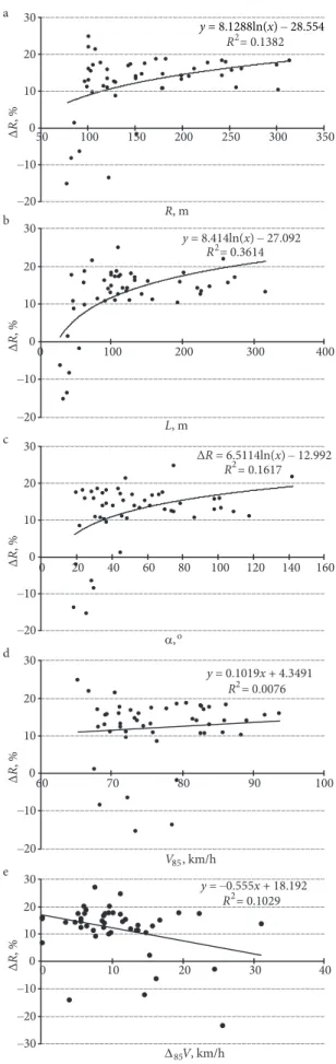
At first, the analysis with the data from the test drives of each direction was performed showing that there were no dependence between ∆R and characteristics of surroun-ding elements as well as speed differential. Therefore, furt-her analysis was conducted with the data from 40 test dri-ves, considering only speed and geometric characteristics of curves. Before the multiple linear regression procedure, the effects of each variable were examined by their indi-vidual scatter plots and indiindi-vidual regressions, as shown in Fig. 2. From this preliminary analysis, it was found that the selected independent variables cannot explain much of the ∆R variability. The curve length has the most signifi-cant impact on ∆R, while the influences of some indepen-dent variables are negligible. The diagrams for curve radius, curve length, deflection angle, operating speed and speed differential (for one direction) are shown in Fig. 2.
Although the selected variables do not explain much of the ∆R variability, some regularities about drivers’ be-havior could be concluded. Generally, drivers tend to adopt a path radius sharper than that of the road align-ment. On average, the critical vehicle path radius is 12% smaller than curve radius. The similar was found by Glen-non and Weaver (1972). According them, the radius of the highway curve was from 1.1 to 1.5 times larger than the critical path radius. The highest range of vehicle path ra-dii was found on sharper curves, as shown in Fig. 2a. On sharp and short curves with small deflection angles, many drivers cut the curve performing path radius greater than centerline curve radius (Figs 2a–2c), in order to make the ride more comfortable. At the same time, sharper curves (radii less than about 150 m) are also related to the highest positive ∆R values of even 25%. Since these are small ra-dii curves, they correspond to lower operating speeds but do not depend on curve length and deflection angle. Such behavior could be explained with steering corrections. In order to comfortably negotiate sharp curves, drivers often underestimate the curvature of the alignment. Somewhere along the curve the mistake is realized and it is usually cor-rected by more or less abrupt turn of the steering wheel which results in path radius smaller than that of the curve. Smaller path radius causes an increase of centripetal ac-celeration and thus an increased demand of side friction. In poor driving conditions and for speeds not adapted to the curve geometry, such steering corrections may re-sult in vehicle instability and they may potentially cause a single-vehicle accident. The radii inconsistencies were observed in curves sharper than about 150 m indicating an increased risk of skidding which may be related to the fact that sharp curves are associated with increased acci-dent rates, as shown in Fig. 1. Differences in radii basically do not depend on the vehicle speed as shown in Fig. 2d. Also, no statistically significant relationship between ∆R and ∆85V was found, as it is shown in Fig. 2e.
The negative impact on the driver’s choice of path ra-dius might have had the absence of spirals or the appli-cation of very short spiral transitions, because the driver failed to adjust both, speed and path radius. So, it would be interesting to analyze the driver’s behavior on sections with transition curves of sufficient length, traditional spi-ral transitions or even some new solutions, for example, general transition curves introduced by Kobryń (2014).
In order to further investigate the influence of the curve radius on radii differences, standard deviations of percentage difference between curve radii and critical path radii of each drive were calculated. The relationship between these standard deviations and curve radii is pre-sented in Fig. 3. It could be noticed that the curve radius does not affect the difference between the curve and each driver’s critical path radius. The average standard devia-tion of percentage radii difference is about 9% with slightly greater standard deviations on sharper curves.
Finally, the stepwise regression was used for determi-nation of the radii differences model. Fig. 2 shows that the approximation with logarithmic form is slightly better than the linear approximation for curve length, deflection angle and curve radius. Therefore, the logarithmic values of these variables were chosen in the multiple linear regression delling. The modelling process resulted in a regression mo-del with only the length of curve L as independent variable:
. (3)
Other proposed independent variables were excluded from the model as it was established they do not contri-bute much to the overall prediction. The model states that the percentage difference between the radius of road align-ment and critical vehicle path radius increases in longer curves. Adjusted coefficient of determination of the model is 0.348 and it indicates that, although there is certain de-pendence between the percentage of the radii difference and curve length, it is very weak and unreliable.
3.2. Analysis of safety margins based on path radii and speeds under real world conditions
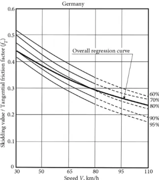
Vehicle stability is an important measure often used for eval-uating design consistency on horizontal curves. The loss of vehicle stability on horizontal curves can be result of exces-sive centripetal force, i.e. it may be due to exceeding the lim-iting values of side friction. Therefore, this safety criterion is based on determining the margin of safety. Two types of safety margins were analyzed in this paper. The first is the difference between maximum permissible side friction and side friction demand, while the second represents the dif-ference between side friction supply and side friction de-mand. Maximum permissible side friction factors are based on skid resistance researches and they are different in each country. However, skid resistance backgrounds do not ex-ist for all countries, because these studies are quite complex and expensive. For example, the skid resistance background in Germany is based on an exhaustive study conducted on different types of pavements and in different driving condi-tions (Lamm et al. 1995). For the safety reasons, the 95th per-centile distribution curve is used to determine the maximum tangential friction factors what means that only 5% of meas-ured values are smaller. The model of Lamm et al. (1995) was used in this paper. Based on the maximum tangential fric-tion factors of selected countries (Germany, France, Sweden, Switzerland and United States), they established an overall regression relationship between the maximum tangential friction factor fT and design speed Vd, km/h:
. (4)
The developed overall curve (4) was compared with friction factors, measured on German highways, as shown in Fig. 4. It could be noticed that the overall regression curve covers between 80% and 90% of the measured va-lues from the German skid resistance inventory.
Fig. 3. The relationship between standard deviations of the percentage radii differences and curve radii
The side friction supply fRsupply is a fraction of tan-gential friction, reduced due to tire-specific influences, as described in Eq (5). Maximum permissible side friction factor can be determined according to side friction supply fRsupply and utilization ratio n (6).
, (5)
. (6)
The utilization ratio n varies between 40% to 60% for rural roads, with respect to the topography and whether it is an existing road. This means that there will still be from 83% to 93% of friction available in the tangential direction for acceleration, deceleration or some evasive maneuvers when driving through curves (Lamm et al. 1995).
Side friction demand fRD is calculated from the basic equation of vehicle stability on horizontal curves, based on operating speed V85, km/h, radius of horizontal curve R, m, and super elevation rate e,%:
. (7)
This formula assumes that drivers follow a path with a radius equal to curve radius and with constant speed. As demonstrated on a real-world experiment, this assumption is not true, i.e. the vehicle path radii are usually smaller than designed radius. Thus, the margins of safety are much less than anticipated. In order to obtain more realistic margins of safety, side friction demand factors were determined for each individual vehicle using the Eq (7), considering vehicle path radii, appropriate curve speeds and actual super ele-vations on curves determined from the road survey. Based on individual side friction demands, the 85th percentile side friction demand fRD85 was determined for each horizontal curve. The 85th percentile side friction demand is the side friction demand that is not exceeded by 85% of drivers. The resulting side friction demands were compared with maxi-mum permissible side friction factors, as shown in Fig. 5. Maximum permissible side friction factors are calculated from the Eq (6), considering the applicable design speed
Vd=60 km/h and utilization ratio for exiting roads n = 60%, as defined by Lamm et al. (1995). One design speed is selec-ted for the whole analyzed road section, so the maximum permissible side friction factor fRperm = 0.196 is unique for all curves, regardless of speeds under real world conditions. Whereas the operating speeds are in excess of the design speed on all analyzed curves, the comparison between side friction demands and side friction supply, determined for operating speeds, is also done. This side friction supply, ba-sed on operating speed, represents maximum available side friction (in terms of the Lamm’s overall regression curve) at pure cornering.
Therefore, in accordance with the side friction factors specified, two different margins of safety are defined. The first margin of safety represents the difference between ma-ximum permissible side friction (based on design speed Vd) and side friction demand (∆fR1 = fRperm – fRD85) (Lamm et al. 1995). The second margin of safety is the difference between side friction supply (based on operating speed V85) and side friction demand (∆fR2 = fRsupply – fRD85).
Based on vehicle stability, the design inconsistency was observed in a great number of curves. It could be no-ticed that the 85th percentile side friction demand factors were greater than permissible values in almost all curves and even in 43% of analyzed curves 85th percentile side friction demand exceeded side friction supply factors. The skidding of test vehicles did not happen, because the overall regression curve corresponds to friction values in the worst conditions (wet and dirty pavement, worn tires). However, these findings point to the danger of skidding when driving at higher percentile speed in poor driving conditions. The side friction demand factors, based on the speeds measu-red on dry pavement, can be compameasu-red with friction values that correspond to wet pavement conditions, as Lamm et al. (1990) indicated that the driver speed choice on two-lane rural highways is not affected by this condition.
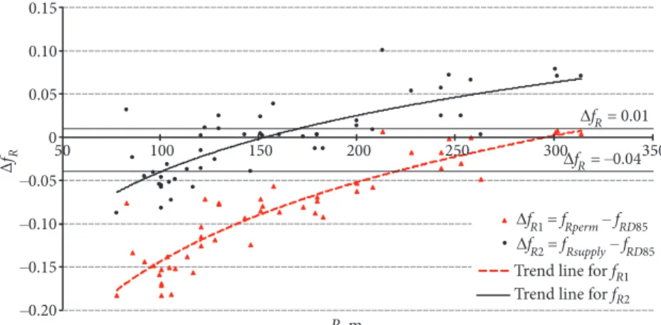
Fig. 6 shows the margins of safety in relation to curve radii, with two sets of safety margins, ∆fR1 and ∆fR2. Since the maximum permissible side friction factors are deter-mined and based on design speed (Vd < V85) and redu-ced by the utilization ratio n, in order to provide a level of skid resistance for safely accommodating the braking and
steering maneuvers, the first set of safety margins is lower than the second one and results in higher negative values. Generally, the greater negative margins of safety can be ob-served on sharper horizontal curves.
Based on accident statistics, Lamm et al. (1995) have defined three design consistency levels: “good design” for R ≥ 350 m, “fair design” for 180 m ≤ R < 350 m, and “poor design” for R < 180 m (Lamm et al. 1995). The limiting val-ues of side friction differences for each consistency level were also specified: “good design” (∆fR1 ≥ 0.01), “fair de-sign” (–0.04 ≤ ∆fR1 < 0.01) and “poor design” (∆fR1 < –0.04). In accordance with Lamm’s design consistency levels, it can be concluded that even 80% of analyzed horizontal curves can be classified as “poor design” while 20% represent “fair design”. In order to establish the marginal radius for “poor” conditions, the trend line that minimizes the squared errors was found (Fig. 6). The limiting radius for “poor” conditions (in terms of ∆fR1 < –0.04), approximately defined from the Fig. 6, is 220 m which is very close to the radius of about 180m determined by Lamm et al. (1995).
Except the analysis of safety margins in terms of ∆fR1, considering the friction reserve for braking and steering maneuvers, the margins of safety for pure cornering, based on operating speeds (∆fR2), were also analyzed. While the ranges for consistency levels, defined by Lamm et al. (1995), exist for ∆fR1, these consistency levels are not relevant for ∆fR2. In the case of ∆fR2, it is interesting to determine the marginal radius above which the curves are safe in terms of ∆fR2=0. According to the trend line defined for ∆fR2, on curves with radii less than about 150 m, the 85th per-centile side friction demands were greater than supplying, while the margins of safety in milder curves were almost always positive. These findings indicate increased risk of skidding for operating speeds on shaper curves with ra-dii less than about 150 m in the case of pure cornering. So, the probability of skidding on curves with radii larger than about 150 m is negligible even in the worst pavement conditions, despite the fact that the operating speeds are greater, because the intensity of decreasing the side fric-tion with the speed is lower for higher speeds.
In general, the analysis of safety margins showed that the sharper curves are more dangerous as higher vehicle
dynamic inconsistencies were observed on smaller radius curves. It is also interesting to notice that the results from Fig. 6 are very similar to the conclusions of accident stud-ies. Most of accident investigations from different parts of the world pointed out an important impact of the curve radius on road safety. Accident analyses showed that in-creasing curve radii cause lower accident frequency with different opinions concerning at which radius the impact decreases, starting with the value of about 200 m (Fig. 1). This accident frequency critical radius of 200 m lies some-where between the marginal radius of 150 m and limiting radius for “poor” conditions of 220 m from the Fig. 6.
This leads to the conclusion that a road design with the use of radii larger than about 200 m would significantly in-crease the road safety. Milder curves are safer than sharper curves due to decreased probability of skidding as confirmed by accident rates. So, in order to improve the road safety, au-thors proposed that curves sharper than 200 m should be avoided on two-lane state roads outside the built-up area. 4. Conclusions
This paper presents the design consistency evaluation on horizontal curves, based on real-life driving data, in terms of the vehicle path radii and operating speeds. The re-search was carried out on a segment of the two-lane state road in Croatia using a GPS device. Specific characteristic of the research as well as the conclusions of the collected data analysis are presented below:
1. In most of the previous instrumented vehicles-based methods for obtaining driving behavior data, all drivers were using the same test vehicle. The data collection methodology used consists of different drivers driving their own cars equip-ped with a GPS device which certainly represents more realis-tic driver behavior data.
2. The differences between critical 15th percentile ve-hicle path and curve radii were observed. Generally, drivers tend to track vehicle path in sharper curvature than that of the road alignment with, on average, 12% lower critical path radius than that of the curve.
3. It was investigated whether the geometric design, speed and speed differential affect the percentage difference between the curve radii and critical 15th percentile vehicle
path radii and no statistically significant correlation was found.
4. Vehicle path radii, lower than curve radii, are ob-served, which means that the current margins of safety are much less than anticipated. More realistic side friction de-mand factors (and thereby margins of safety) were deter-mined based on the vehicle path radii, speeds under real world conditions and real super elevation rates. 85th per-centile side friction demands were greater than permissi-ble values (determined using the design speed Vd and uti-lization ratio n = 60%) in almost all curves and in 43% of analyzed curves they exceeded supply side friction factors (determined based on Lamm’s overall regression curve using the operating speed V85).
5. The improvement of design consistency measure re-garding to the vehicle stability is proposed in terms of lower curve radius. Since the critical vehicle path radius 12% lower than curve radius was observed, it is proposed to use this va-lue when calculating the margin of safety. Smaller vava-lues of curve radii would result in lower margins of safety and thus inconsistencies would be easier detected and eliminated. Ho-rizontal curves of the final road design would hence repre-sent the satisfactory level of consistency even in real condi-tions for the majority of drivers. Designing horizontal curves that are in accordance with the driver behavior is a base to reaching a better design and safer roads.
6. Two types of safety margins were analyzed: ∆fR1 and ∆fR2. Considering the difference between maximum per-missible side friction and side friction demand (∆fR1), the limiting radius for “poor” conditions (in terms of Lamm’s consistency levels) was determined to about 220 m. Ana-lyzing the difference between supply side friction and 85th percentile side friction demand (∆fR2), negative margins of safety were observed on curves sharper than about 150 m while on milder curves they were almost always positive, despite the fact that the operating speeds are greater. Both radii are very close to accident frequency critical radius be-low which higher accident rates are observed.
7. Curves with radii less than 200 m should be avoided on two-lane state roads outside the built-up area due to in-creased risk of skidding for operating speeds.
References
Cafiso, S.; La Cava, G. 2009. Driving Performance, Alignment Consistency, and Road Safety Real-World Experiment, Trans-portation Research Record 2102: 1–8.
http://dx.doi.org/10.3141/2102-01
Carlson, P. J.; Burris, M.; Black, K.; Rose, E. R. 2005. Compari-son of Radius-Estimating Techniques for Horizontal Curves, Transportation Research Record 1918: 76–83.
http://dx.doi.org/10.3141/1918-10
Castro, M.; Pardillo-Mayora, J. M.; Jurado, R. 2013. Development of a Local Operating Speed Model for Consistency Analy-sis Integrating Laser, GPS and GIS for Measuring Vehicles Speed, The Baltic Journal of Road and Bridge Engineering 8(4): 281–288. http://dx.doi.org/10.3846/bjrbe.2013.36
ERA-NET ROAD 2012. Safety at the Heart of Road Design. Final Report of the ERA-NET programme.
Glennon, J. C.; Weaver, G. D. 1972. Highway Curve Design for Safe Vehicle Operations, Highway Research Record 390: 15–26. Hassan, Y.; Sayed, T.; Tabernero, V. 2001. Establishing Practi-cal Approach for Design Consistency Evaluation, Journal of Transportation Engineering 127(4): 295–302.
http://dx.doi.org/10.1061/(ASCE)0733-947X(2001)127:4(295) Kobryń, A. 2014. New Solutions for General Transition Curves,
Journal of Surveying Engineering 140(1): 12–21. http://dx.doi.org/10.1061/(ASCE)SU.1943-5428.0000113 Krebs, H. G.; Kloeckner, J. H. 1977. Investigations of the Effect of
Highway and Traffic Conditions Outside Built-Up Areas on Ac-cident Rates, Forschung Straßenbau und Straßenverkehrstechnik [Research Road Construction and Traffic Technique] 223. Lamm, R.; Psarianos, B.; Mailaender, T. 1999. Highway Design and
Traffic Safety Engineering: Handbook. McGraw Hill. 1088 p. Lamm, R.; Psarianos, B.; Choueiri, E. M.; Soilemezoglou, G. 1995.
A Practical Safety Approach to Highway Geometric Design International Case Studies: Germany, Greece, Lebanon, and the United States, in Proc. of the International Symposium on Highway Geometric Design Practices, August 30 – September 1, 1995, Texas Transportation Institute, Boston, Massachu-setts, 9: 1–9.
Lamm, R.; Choueiri, E. M.; Goyal, P. B.; Mailaender, T. 1990. Comparison of Operating Speeds on Dry and Wet Pavements of Two-Lane Rural Highways, Transportation Research Record 1280: 199–207.
Modeling Operating Speed: Synthesis Report. 2011. Transporta-tion Research Board. 136 p.
Nicholson, A. 1998. Superelevation, Side Friction, and Roadway Consistency, Journal of Transportation Engineering 124(5): 411–418.
http://dx.doi.org/10.1061/(ASCE)0733-947X(1998)124:5(411) Pérez-Zuriaga, A. M.; Camacho-Torregrosa, F. J.; García, A. 2013.
Tangent-to-Curve Transition on Two-Lane Rural Roads Based on Continuous Speed Profiles, Journal of Transporta-tion Engineering 139(11): 1048–1057.
http://dx.doi.org/10.1061/(ASCE)TE.1943-5436.0000583 PIARC Technical Committee on Road Safety 2003. Road Safety
Manual. World Road Association. 602 p.
Raff, M. S. 1953. Interstate Highway Accident Study, Highway Research Board Bulletin 74: 18–45. Traffic Accident Studies Washington D.C.
Said, D.; Halim, A. E.; Hassan, Y. 2010. Methodology for Driver Behaviour Data Collection and Analysis for Integration in Ge-ometric Design of Highways [CD-ROM], in D. W. Harwood, A. García (Eds.). Proc. of the 4th International Symposium on
Highway Geometric Design, June 1–5, 2010, Valencia, Spain. Torbic, D. J.; Harwood, D. W.; Gilmore, D. K.; Pfefer, R.; Neuman,
T. R.; Slack, K. L.; Hardy, K. K. 2004. Guidance for Implementa-tion of the AASHTO Strategic Highway Safety Plan: A Guide for Reducing Collisions on Horizontal Curves, NCHRP Report 500 Series, Vol. 7, Transportation Research Board, Washington, D.C. World Health Organization 2013. Global Status Report on Road
Safety 2013 – Supporting a Decade of Action. Available from Internet:<http://www.who.int/violence_injury_prevention/ road_safety_status/2013/en/>