American Options
The distinctive feature of an American option is its early exercise privilege, that is, the holder can exercise the option prior to the date of expiration. Since the additional right should not be worthless, we expect an American option to be worth more than its European counterpart. The extra premium is called theearly exercise premium.
First, we would like to recall some of the pricing properties of American options discussed in Sec. 1.2. The early exercise of either an American call or American put leads to the loss of insurance value associated with holding of the option. For an American call, the holder gains on the dividend yield from the asset but loses on the time value of the strike price. There is no advantage to exercise an American call prematurely when the asset received upon early exercise does not pay dividends. In this case, the American call has the same value as that of its European counterpart. By dominance argument, we have shown that an American option must be worth at least its corresponding intrinsic value, namely, max(S−X,0) for a call and max(X −S,0) for a put, where S and X are the asset price and strike price, respectively. While put-call parity relation exists for European options, we can only obtain lower and upper bounds on the difference of American call and put option values. When the underlying asset is dividend paying, it may become optimal for the holder to exercise prematurely an American call option when the asset price S rises to some critical asset value, called the optimal exercise price. Since the loss of insurance value and time value of the strike price is time dependent, the optimal exercise price depends on time to expiry. For a longer-lived American call option, the optimal exercise price should assume a higher value so that larger dividends are received to compensate for the greater loss on time value of strike. When the underlying asset pays continuous dividend yield, the collection of these optimal exercise prices for all times constitutes a continuous curve, which is commonly called theoptimal exercise boundary. For an American put option, the early exercise leads to some gain on time value of strike. Therefore, when the riskless interest rate is positive, there always exists an optimal exercise price below which it becomes optimal to exercise the American put prematurely.
The optimal exercise boundary of an American option is not known in advance but has to be determined as part of the solution process of the pricing
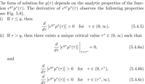
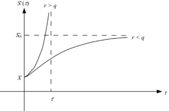
model. Since the boundary of the domain of an American option model is a free boundary, the valuation problem constitutes a free boundary value problem. In Sec. 5.1, we present the characterization of the optimal exercise boundary at infinite time to expiry and at the moment immediately prior to expiry. The optimality condition in the form of smooth pasting of the option value curve with the intrinsic value line is derived. When the underlying asset pays discrete dividends, the early exercise of the American call may become optimal only at time right before a dividend date. Since the early exercise policy becomes relatively simple, we manage to derive closed form price formulas for American calls on an asset that pays discrete dividends. We also discuss the optimal exercise policy of American put options on a discrete dividend paying asset.
In Sec. 5.2, we present two pricing formulations of American options, namely, the linear complementarity formulaton and the optimal stopping formulation. We show how the early exercise premium can be expressed in terms of the exercise boundary in the form of an integral and examine how the determination of the optimal exercise boundary is resorted to the solution of an integral equation. The early exercise premium can be interpreted as the compensation paid to the holder when the early exercise right is forfeited. The early exercise feature can be combined with other path dependent fea-tures in an option contract. We examine the impact of the barrier feature on the early exercise policies of American barrier options. Also, we obtain the analytic price formula for the Russian option, which is essentially a perpetual American lookback option.
In general, analytic price formulas are not available for American op-tions, except for a few special types. In Sec. 5.3, we present several analytic approximation methods for estimating the price of an American option. One approximation approach is to limit the exercise right such that the Ameri-can option is exercisable only at a finite number of time instants. The other method is the solution of the integral equation of the exercise boundary by a recursive integraton method. The third method, called the quadratic approx-imation approach, is based on the reduction of the Black-Scholes equation to an ordinary differential equation whose domain boundary is determined by maximizing the value of the option.
The modeling of a financial derivative with voluntary right on resetting certain terms in the contract, like resetting the strike price to the prevailing asset price, also constitutes a free boundary value problem. In Sec. 5.4, we construct the pricing model for the reset-strike put option and examine the optimal reset strategy adopted by the option holder. Unlike the American early exercise right, the right to reset may not be limited to only one time. We also examine the pricing behaviors of multi-reset put options. Interestingly, when the right to reset is allowed to be infinitely often, the multi-reset put option becomes a European lookback option.
5.1 Characterization of the optimal exercise boundaries
The characteristics of the optimal early exercise policies of American options depend critically on whether the underlying asset is non-dividend paying or dividend paying (discrete or continuous). Throughout our discussion, we assume that the dividends are known in advance, both in amount and time of payment. In this section, we would like to give some detailed quantitative analysis of the properties of the early exercise boundary. We show that the optimal exercise boundary of an American put, with continuous dividend yield or zero dividend, is acontinuous decreasing function of time of expiry τ. However, the optimal exercise boundary for an American put on an asset which pays discrete dividends may or may not have jumps of discontinuity, depending on the size of the discrete dividend payments. For an American call on an asset which pays a continuous dividend yield, we explain why it becomes optimal to exercise the call at sufficiently high value ofS. The corresponding optimal exercise boundary is acontinuous increasing function ofτ. When the underlying asset of an American call pays discrete dividends, optimal early exercise of the American call may occur only at those times immediately before the asset goes ex-dividend. Additional conditions required for optimal early exercise include (i) the discrete dividend is sufficiently large relative to the strike price, (ii) the ex-dividend date is fairly close to expiry and (iii) the asset price level prior to the dividend date is higher than some threshold value. Since exercise possibilities are limited to a few discrete dividend dates, the price formula for an American call on an asset paying known discrete dividends can be obtained by relating the American call option to a European compound option.
Besides the value matching condition of the American option value across the optimal exercise boundary, the delta of the option value are also contin-uous across the boundary. Thissmooth pasting condition is a result derived from maximizing the American option value among all possible early exercise policies (see Sec. 5.1.2).
5.1.1 American options on an asset paying dividend yield
First, we consider the effects of continuous dividend yield (at the constant yield q > 0) on the early exercise policy of an American call. When the asset valueS is exceedingly high, it is almost certain that the European call option on a continuous dividend paying asset will be in-the-money at expiry. Its value then behaves almost like the asset but without its dividend income minus the present value of the strike price X. When the call is sufficiently deep in-the-money, by observing that
N( ˆd1)∼1 and N( ˆd2)∼1
c(S, τ)∼e−qτS−e−rτX when SX. (5.1.1) The price of this European call may be below the intrinsic value S −X at a sufficiently high asset value, due to the presence of the factore−qτ in front of S. While it is possible that the value of a European option stays below its intrinsic value, the holder of an American option with embedded early exercise right would not allow the value of his option to become lower than the intrinsic value. Hence, at a sufficiently high asset value, it becomes optimal for the American option on a continuous dividend paying asset to be exercised prior to expiry, avoiding its value to drop below the intrinsic value if unexercised.
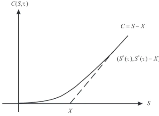
Fig. 5.1The solid curve shows the price functionC(S, τ) of an American call on an asset paying continuous divi-dend yield. The price curve touches the dotted intrinsic value line tangentially at the point (S∗(τ), S∗(τ)−X),
where S∗(τ) is the optimal exercise price. When S ≥ S∗(τ), the American call value becomes S−X.
In Fig. 5.1, the American call option price curve C(S, τ) touches tan-gentially the dotted line representing the intrinsic value of the call at some optimal exericse price S∗(τ). Note that the optimal exericse price has
de-pendence on τ, the time to expiry. The tangency behavior of the Ameri-can price curve atS∗(τ) (continuity of delta value) will be explained in the
next subsection. When S ≥ S∗(τ), the American call value is equal to its
intrinsic value S−X. The collection of all these points (S∗(τ), τ), for all
τ ∈ (0, T], in the (S, τ)-plane constitutes the optimal exercise boundary. The American call option remains alive only within thecontinuation region
{(S, τ) : 0≤S < S∗(τ),0< τ ≤T}. The complement is called the stopping region, inside which the American call should be optimally exercised (see Fig. 5.2).
optimal exercise boundary continuation region stopping region
s
*( )
t
t
(0+ S* )s
*( )
t
Fig. 5.2An American call on an asset paying continu-ous dividend yield remains alive inside the continuation region {(S, τ) : S ∈ [0, S∗(τ)), τ ∈ (0, T]}. The optimal
exercise boundaryS∗(τ) is a continuous increasing
func-tion ofτ.
Under the assumption of continuity of the asset price path and dividend yield, we expect that the optimal exercise boundary should also be a con-tinuous function of τ, for τ >0. While a rigorous proof of the continuity of
S∗(τ) is rather technical, a heuristic argument is provided below. Assume the contrary, supposeS∗(τ) has a downward jump asτ decreases across the time instantbτ. Assume that the asset priceSatbτ satisfiesS∗(bτ−)< S < S∗(τb+), the American call option value is strictly above the intrinsic value S−X
at bτ+ since S < S∗(τb+) and becomes equal to the intrinsic value S−X at
b
τ− since S > S∗( b
τ−). The discrete downward jump in option value across b τ
would lead to an arbitrage opportunity.
5.1.2 Smooth pasting condition
We would like to examine the smooth pasting condition (tangency condition) along the optimal exercise boundary for an American call on a continuous dividend paying asset. At S = S∗(τ), the value of the exercised American
call isS∗(τ)−X. This is termed value matching condition:
C(S∗(τ), τ) =S∗(τ)−X. (5.1.2)
Suppose S∗(τ) were a known continuous function, the pricing model
be-comes a boundary value problem with a time dependent boundary. However, in the American call option model,S∗(τ) is not known in advance. Rather, it
must be determined as part of the solution. An additional auxiliary condition has to be prescribed alongS∗(τ) so as to reflect the nature of optimality of the exercise right embedded in the American option.
We follow Merton’s (1973; Chap. 1) argument to show the continuity of the delta of option value of an American call at the optimal exercise price S∗(τ). Let f(S, τ;b(τ)) denote the solution to the Black-Scholes equation in the domain {(S, τ) : S ∈ (0, b(τ)), τ ∈ (0, T]}, where b(τ) is a known boundary. The holder of the American call chooses an early exercise policy which maximizes the value of the call. Using such argument, the American call value is given by
C(S, τ) = max
{b(τ)} f(S, τ;b(τ)) (5.1.3)
for all possible continuous functions b(τ). For fixed τ, for convenience, we writef(S, τ;b(τ)) asF(S, b), where 0≤S ≤b. It is observed thatF(S, b) is a differentiable function, concave in its second argument. Further, we write h(b) =F(b, b) which is assumed to be a differentiable function ofb. For usual American call option,h(b) = b−X. The total derivative ofF with respect tob along the boundaryS =bis given by
dF db = dh db = ∂F ∂S(S, b) S=b+ ∂F ∂b(S, b) S=b, (5.1.4) where the property ∂S
∂b = 1 alongS=bhas been incorporated. Letb ∗
be the critical value ofb which maximizesF. Whenb=b∗, we have ∂F
∂b(S, b ∗
) = 0 as the first derivative condition at a maximum point. On the other hand, from the exercise payoff function of the American call option, we have
dh db b=b∗ = d db(b−X) b=b∗ = 1. (5.1.5) Putting the results together, we obtain
∂F ∂S(S, b ∗ ) S=b∗ = 1. (5.1.6)
Note that the optimal choice b∗(τ) is just the optimal exercise price S∗(τ). The above condition can be expressed in an alternative form as
∂C ∂S(S
∗
(τ), τ) = 1. (5.1.7) Condition (5.1.7) is commonly called thesmooth pasting or tangency condi-tion. The two conditions (5.1.2) and (5.1.7), respectively, reveal thatC(S, τ) and ∂C
∂S(S, τ) are continuous across the optimal exercise boundary (see Fig. 5.1).
The smooth pasting condition is applicable to all types of American put options. For an American put option, the slope of the intrinsic value line is
∂P ∂S(S
∗
(τ), τ) =−1. (5.1.8) An alternative proof of the above smooth pasting condition is outlined in Problem 5.5.
5.1.3 Optimal exercise boundary for an American call
Consider an American call on a continuous dividend paying asset, the opti-mal exercise boundary S∗(τ) is a continuous increasing function of τ. The increasing property stems from the fact that the loss of time value of strike is more significant for a longer-lived American call so that the call must be deeper-in-the-money in order to induce early exercise decision. In addi-tion, the compensation from the dividend received from the asset is higher whereas the loss of insurance value associated with holding of the call option becomes lower (chance of expiring out-of-the-money becomes lower). Hence, the American call should be exercised at a higher optimal exericse priceS∗(τ) compared to its shorter-lived counterpart.
The increasing property of S∗(τ) can also be explained by relating to the increasing property of the price curve C(S, τ) as a function of τ [see Eq. (1.2.5a)]. The option price curve of a longer-lived American call plotted againstSalways stays above that of its shorter-lived counterpart. The upper price curve corresponding to the longer-lived option cuts the intrinsic value line tangentially at a higher critical asset valueS∗(τ).
Moreover, it is obvious from Fig. 5.1 that the price curve of an American call always cuts the intrinsic value line at a critical asset value greater than X. Hence, we haveS∗(τ)≥X forτ ≥0. Alternatively, assume the contrary, suppose S∗(τ) < X, then the early exercise proceed S∗(τ)−X becomes negative. Since the early exercise privilege cannot be a liability, the possibility S∗(τ)< X is ruled out and soS∗(τ)≥X.
Next, we present the analysis of the asymptotic behaviors of S∗(τ) at τ →0+ andτ → ∞.
Asymptotic behavior of S∗(τ)close to expiry
Whenτ →0+ and S > X, by the continuity of the call price function, the
call value tends to the terminal payoff value so thatC(S,0+) =S−X. If the
American call is alive, then the call value satisfies the Black-Scholes equation. By substituting the above call value into the Black-Scholes equation, given that (S, τ) lies in the continuation region, we have
∂C ∂τ τ=0+ =σ 2 2 S 2∂ 2C ∂S2 τ=0+ + (r−q)S∂C ∂S τ=0+ −rC τ=0+ = (r−q)S−r(S−X) =rX−qS. (5.1.9) Suppose ∂C ∂τ(S,0
+)<0,C(S, τ) becomes less thanC(S,0) =S−X (intrinsic
contradiction since the American call value is always above the intrinsic value. Therefore, we must have ∂C
∂τ (S,0
+) ≥0 in order that the American call is
kept alive until the time close to expiry. The value ofS at which ∂C ∂τ (S,0
+)
changes sign is S = r
qX. Also, r
qX lies in the intervalS > X only when q < r. We consider the two separate cases,q < randq≥r.
1. q < r
At time immediately prior to expiry, we argue that the American call will be kept alive when S < r
qX.This is because within a short time interval δtprior to expiry, the dividendqSδtearned from holding the asset is less than the interest rXδt earned from depositing the amountX in a bank at the riskless interest rate r. The above observation is consistent with positivity of ∂C ∂τ (S,0 +) when S < r qX. When S > r qX, the American call should be exercised since the negativity of ∂C
∂τ(S,0
+
) would lead to the violation of the condition that the American call value must be above the intrinsic value S−X. Hence, for q < r, the optimal exercise price S∗(0+) is given by the asset value at which ∂C
∂τ(S,0
+) changes sign. We
then obtain
S∗(0+) = r
qX. (5.1.10a)
In particular, whenq= 0,S∗(0+) becomes infinite. Furthermore, since S∗(τ) is known to be a monotonically increasing function of τ, we then deduce that S∗(τ)→ ∞for all values of τ. This result is consistent with the well known fact that it is always non-optimal to exercise an American call on a non-dividend paying asset prior to expiry.
2. q≥r
When q ≥r, r
qX becomes less thanX and so the above argument has to be modified. First, we show that S∗(0+) cannot be greater than X. Assume the contrary, suppose S∗(0+) > X so that the American call
is still alive when X < S < S∗(0+) at time close to expiry. Given the
combined conditions: q ≥r and S > X, it is observed that the loss in dividend amountqSδtnot earned is more than the interest amountrXδt earned if the American call is not exercised within a short time intervalδt prior to expiry. This represents a non-optimal early exercise policy. Hence, we must haveS∗(0+)≤X. Together with the properties thatS∗(τ)≥X for τ >0 and S∗(τ) is a continuous increasing function of τ, we deduce that for q≥r,
In summary, the optimal exercise price S∗(τ) of an American call on a continuous dividend paying asset at time close to expiry is given by
lim τ→0+S ∗ (τ) = r qX q < r X q≥r =Xmax 1,r q . (5.1.11) At expiry τ = 0, the American call option will be exercised whenever S≥X and so S∗(0) =X. Hence, for q < r, there is a jump of discontinuity ofS∗(τ) atτ = 0.
Asymptotic behavior of S∗(τ)at infinite time to expiry
SinceS∗(τ) is a monotonic increasing function ofτ, the lower bound for the optimal exercise boundaryS∗(τ) forτ > 0 is given by lim
τ→0+S
∗
(τ).It would be interesting to explore whether lim
τ→∞S ∗
(τ) has a finite bound or otherwise. An option with infinite time to expiration is called aperpetual option. The determination of lim
τ→∞S ∗
(τ) is related to the analysis of the price function of corresponding perpetual American option.
Let C∞(S;X, q) denote the price of an American perpetual call option with strike priceX and on an asset which pays a continuous dividend yield q. The value of a perpetual option is seen to be insensitive to temporal rate of change so that the Black-Scholes equation is reduced to the following ordinary differential equation σ2 2 S 2d 2C ∞ dS2 + (r−q)S dC∞ dS −rC∞= 0, 0< S < S ∗ ∞, (5.1.12a) whereS∞∗ is the optimal exercise price at which the perpetual American call option should be exercised. Note thatS∗∞is independent ofτ and it is simply the asymptotic value lim
τ→∞S ∗
(τ). The boundary conditions for the pricing model of the perpetual American call are
C∞(0) = 0 and C∞(S∞) =∗ S∞∗ −X. (5.1.12b) We let f(S;S∗
∞) denote the solution to Eqs. (5.1.12a,b) for a given value of S∗
∞. Since Eq. (5.1.12a) is a linear equi-dimensional ordinary differential equation, its general solution is of the form
f(S;S∞∗ ) =c1Sµ++c2Sµ−, (5.1.13)
wherec1andc2are arbitrary constants,µ+andµ−are the respective positive and negative roots of the auxiliary equation:
σ2 2 µ
2+ (r−q−σ 2
2 )µ−r= 0. (5.1.14) Sincef(0;S∞) = 0, we must have∗ c2= 0. Applying the boundary condition
atS∞, we have∗ f(S∗∞;S ∗ ∞) =c1S∞∗µ+ =S ∗ ∞−X, (5.1.15)
thus giving c1= S∗∞−X S∗µ+ ∞ . (5.1.16) The solutionf(S;S∗
∞) is now reduced to the form f(S;S∞∗ ) = (S ∗ ∞−X) S S∗ ∞ µ+ , (5.1.17a) where µ+= −(r−q−σ22) + q (r−q−σ22)2+ 2σ2r σ2 >0. (5.1.17b)
To complete the solution,S∞∗ has yet to be determined. We findS ∗
∞ by max-imizing the value of the perpetual American call option among all possible optimal exercise prices, that is,
C∞(S;X, q) = max {S∗ ∞} (S∞∗ −X) S S∗ ∞ µ+ . (5.1.18) The use of calculus shows thatf(S;S∗
∞) is maximized when S∞∗ = µ+ µ+−1 X. (5.1.19) Suppose we writeS∗ ∞,C= µ+ µ+−1
X, then the value of the perpetual Ameri-can call takes the form
C∞(S;X, q) = S∗ ∞,C µ+ S S∗ ∞,C !µ+ . (5.1.20) It can be easily verified that the above solution also satisfies the smooth pasting condition: dC∞ dS S=S∗ ∞,C = 1. (5.1.21)
One may solve for S∗
∞,C by applying the smooth pasting condition directly without going through the above maximization procedure. Indeed, the appli-cation of the smooth pasting condition implicity incorporates the procedure of taking the maximum of the option values among all possible choices of S∞,C∗ .
5.1.4 Put-call symmetry relations
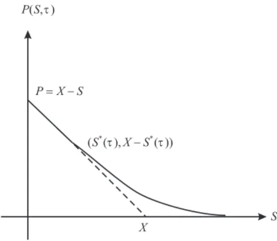
The behaviors of the optimal exercise boundary for an American put option on a continuous dividend paying asset can be inferred from those of the call counterpart once the put-call symmetry relations between their price functions and optimal exercise prices are established. The plot of the price functionP(S, τ) of an American put againstS is shown in Fig. 5.3.
Fig. 5.3 The solid curve shows the price function of an American put at a given time to expiryτ. The price curve touches the dotted intrinsic value line tangentially at the point (S∗(τ), X−S∗(τ)), where S∗(τ) is the optimal
ex-ercise price. When S ≤ S∗(τ), the American put value
becomesX−S.
We may consider an American call option as providing the right to ex-changeX dollars of cash for one unit of stock which is worthSdollars at any time during the option’s life. If we take asset one to be the stock, asset two to be the cash, then asset one and asset two have dividend yieldqandr, respec-tively. The above call option can be considered as an exchange option which exchanges asset two for asset one. Similarly, we may consider an American put option as providing the right to exchange one unit of stock which is worth
S dollars forX dollars of cash at any time. What would happen if we inter-change the role of stock and cash in the American put option? Now, this new American put can be considered to be equivalent to the usual American call since both options confer the same right of exchanging cash for stock to their holders. If we use P(S, τ;X, r, q) to denote the price function of the usual American put, then the price function of the modified American put (after interchanging the role of stock and cash) is given byP(X, τ;S, q, r), whereS
andX are interchanged and so dorandq. Since the modified American put is equivalent to the usual American call, we then have
C(S, τ;X, r, q) =P(X, τ;S, q, r). (5.1.22) This symmetry between the price functions of American call and put is called theput-call symmetry relation.
Next, we would like to establish the put-call symmetry relation for the optimal exercise prices for American put and call options. Let S∗P(τ;r, q) and SC∗(τ;r, q) denote the optimal exercise boundary for the American put and call options on a continuous dividend paying stock, respectively. When S =SC∗(τ;r, q), the call owner is willing to exchange X dollars of cash for one unit of stock which is worth SC∗ dollars or one dollar of cash for X1 units of stock which is worth S
∗ C
X dollars. Similarly, when S = S ∗
P(τ;r, q), the put owner is willing to exchange 1
S∗ P
units of stock which is worthone dollar for X
S∗ P
dollars of cash. If both of these American call and put options can be considered as exchange options and the roles of cash and stock are interchangeable, then the corresponding put-call symmetry relation for the optimal exercise prices is deduced to be
SC∗(τ;r, q) = X
2
S∗
P(τ;q, r)
. (5.1.23)
A mathematical proof of symmetry relation (5.1.22) can be established quite easily (see Problem 5.7). Indeed, more complicated symmetry relations between the price functions of American call and put options can be derived (see Problems 5.8–5.9).
Behavior of S∗
P(τ) near expiry
From Eq. (5.1.23) and the monotonically increasing property of S∗ C(τ), we can deduce thatS∗
P(τ) is a monotonically decreasing function ofτ. Since Eq. (5.1.23) remains valid asτ →0+, the lower bound forS∗
P(τ) is given by lim τ→0+S ∗ P(τ;r, q) = X2 lim τ→0+S ∗ C(τ;q, r) = X 2 Xmax 1,qr=Xmin 1,r q . (5.1.30) From Eq. (5.1.30), we observe that whenq≤r, we have lim
τ→0+S
∗
P(τ) =X. Now, even whenq= 0,S∗
P(τ) is non-zero sinceS ∗
P(τ) is a continuous decreas-ing function ofτ forτ >0 and its lower bound equals X. Hence, it is always optimal to exercise an American put even when the underlying asset pays no dividend. On the other hand, at zero interest rate, lim
τ→0+S
∗
P(τ) becomes zero. It then follows thatS∗P(τ) = 0 forτ >0 sinceS∗P(τ) is a decreasing function
ofτ. Therefore, it is never optimal to exercise an American put prematurely when the interest rate is zero. From financial intuition, such a conclusion is obvious since there is no time value gained on X from the early exercise of the American put when there is null interest.
The quest for more refined asymptotic behaviors of S∗
P(τ) whenτ →0+ poses great mathematical challenges. Evanset al. (2002) show that at time close to expiry the optimal exercise boundary is parabolic when q > r but it becomes parabolic-logarithmic when q ≤r. The asymptotic expansion of SP∗(τ) asτ →0+ takes the following forms
(i) 0≤q < r SP∗(τ)∼X−Xσ s τln σ2 8πτ(r−q)2 (5.1.31a) (ii) q=r SP∗(τ)∼X−Xσ s 2τln 1 4√πqτ (5.1.31b) (iii) q > r SP∗(τ)∼ r qX(1−σα √ 2τ). (5.1.31c) Here, αis a numerical constant which satisfies the following transcen-dental equation −α3eα2 Z ∞ α e−u2du= 1−2α 2 4 . (5.1.31d) Behavior of S∗
P(τ) at infinite time to expiry
Following a similar derivation procedure as that for the perpetual American call option, the price of the perpetual American put option can be deduced to be P∞(S;X, q) =−S ∗ ∞,P µ− S S∗ ∞,P !µ− . (5.1.32) Here, S∗
∞,P denotes the optimal exercise price at infinite time to expiry and its value is equal to
S∞,P∗ = µ− µ−−1 X, (5.1.33a) where µ−= −(r−q−σ2 2)− q (r−q−σ2 2 )2+ 2σ2r σ2 <0. (5.1.33b)
One can verify easily that S∞,P∗ (r, q) = X2 S∗ ∞,C(q, r) , (5.1.34)
a result that is consistent with the relation given in Eq. (5.1.23). 5.1.5 American call options on an asset paying single dividend It has been explained in Sec. 1.2 that when an asset pays discrete dividend payments, the asset price declines by the same amount as the dividend right after the dividend date if there are no other factors affecting the income pro-ceeds. Empirical studies show that the relative decline of the stock price as a proportion of the amount of the dividend is shown to be not meaningfully different from one. For simplicity, we assume that the asset price falls by the same amount as the discrete dividend. An option is said to be dividend protectedif the value of the option is invariant of the choice of the dividend policy. This is done by adjusting the strike price in relation to the dividend amount. Here, we consider the effects of discrete dividends on the early exer-cise policy of American options which are not protected against the dividend, that is, the strike price is not marked down (for calls) or marked up (for puts) by the same amount as the dividend.
Early exercise policies
Since the holder of an American call on an asset paying discrete dividends will not receive any dividends between successive dividend dates, it is never optimal to exercise the American call on any non-dividend paying date. For those times between dividend dates, the early exercise right is non-effective. If the American call were exercised at all, the possible choices of exercise times are those instants immediately before the asset goes ex-dividend. As a result, he owns the asset right before the asset goes ex-dividend and receives the dividend in the next instant. We explore the conditions under which the holder of such American call would optimally choose to exercise his option.
In the following discussion, it is more convenient to characterize the time dependence of the optimal exercise boundary using the calendar timet. We consider an American call on an asset which pays only one discrete dividend of deterministic amountD at the known dividend date td. The generalization to multi-dividend models can be found in Problems 5.15-17. Let S−d(S+d) denote the asset price at timet−d(t+d) which is immediately before (after) the discrete dividend datetd. If the American call is exercised att−d, the call value becomes Sd− −X. Otherwise, the asset price drops to Sd+ = S−d −D right after the asset goes ex-dividend. Since there is no further discrete dividend after timetd, the American price function behaves like that of its European counterpart for t > t+d. To preclude arbitrage opportunities, the call price function must be continuous across the ex-dividend instant since the holder
of the call option does not receive any dividend payment on the dividend date (unlike holding the asset).
From Eq. (1.2.11), the lower bound of the American call value at t+d is Sd+−Xe−r(T−t+d),whereT−t+
d is the time to expiry. As far as time to expiry is concerned, the quantitiesT−td, T−t+d andT−t−d are considered equal. By virtue of the continuity of the call value across the dividend date, the lower bound for the call value at timet−d should also be equal toS+d −Xe−r(T−td)=
(S−d −D)−Xe−r(T−td).Note that the lower bound for the call value att−
d is driven down byD in anticipation of the known discrete dividend amount D in the next instant. Now, it may occur that the lower bound value at t−d becomes less than the exercise payoff ofSd−−X whenD is sufficiently large. We compare the following two quantities: exercise payoff E =S−d −X and lower bound of the call valueB= (Sd−−D)−Xe−r(T−td).SupposeE≤B,
that is
S−d −X ≤(Sd−−D)−Xe−r(T−td) or D≤X [1−e−r(T−td)], (5.1.35)
then it is never optimal to exercise the American call. This is because at any value of asset priceSd− the call is worth more when it is held than exercised. However, when the discrete dividend D is deep enough, in particularD > X[1−e−r(T−td)], then it may become optimal to exercise at t−
d when the asset price S−d is above some threshold value. This requirement on D gives one of the necessary conditions for the commencement of early exercise. The dividend amountD must be sufficiently deep to offset the loss in the time value of the strike price, where the loss is given byX[1−e−r(T−td)].
LetCd(S, t) denote the price function of the one-dividend American call option with the calendar timetas the time variable. By virtue of the conti-nuity property of the call value across the dividend date, we have
Cd(S − d, t − d) =c(S − d −D, t + d), (5.1.36)
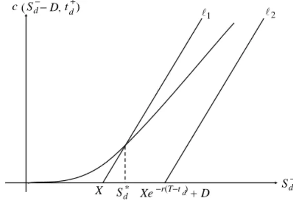
where c(S−d −D, t+d) is the European call price given by the Black-Scholes formula with asset priceSd−−Dand calendar timet+d. To better understand the decision of early exercise att−d, we plot the call price function, the exercise payoffE(corresponds to line`1:E=S−d −X) and the lower bound valueB (corresponds to line`2:B=S
−
d −D−Xe
−r(T−td)) versus the asset priceS−
d (see Fig. 5.4). The exercise payoff linel1 lies to the left of the lower bound
value line l2 when D > X[1−e−r(T−td)]. Now, the call price curve may
intersect (not tangentially) the exercise payoff line l1 at some critical asset
price S∗
d, which is given by the solution to the following algebraic equation c(Sd−−D, td) =Sd−−X. (5.1.37) It can be shown mathematically that when D ≤X[1−e−r(T−td)], there is
no solution to Eq. (5.1.37), a result that is consistent with the necessary condition onD discussed earlier (see also Problem 5.13). When the discrete
dividend is sufficiently deep such that D > X[1−e−r(T−td)], the American
call remains alive beyond the dividend date only ifSd− < S∗
d. WhenS − d is at or aboveS∗
d, the call should be optimally exercised att −
d. Hence, the American call price at timet−d is given by
Cd(S−d, t−d) = c(S−d −D, t+d) when S−d < S∗ d Sd−−X when S−d ≥S∗ d. (5.1.38) If the American call is not optimally exercised att−d, then its value remains unchanged as time lapses across the dividend date. Note that S∗
d depends on D, which decreases in value when D increases (see Problem 5.13). This agrees with the financial intuition that the propensity of optimal early ex-ercise becomes higher (corresponding to a lower value of S∗
d) with deeper discrete dividend payment.
−D, (Sd− td+) c X 1 l l2 d S− d S∗ Xe−r(T−t )d+ D
Fig. 5.4The curve representing the European call price functionV =c(S–d−D, t+d) falls below the exercise payoff line`1:E =S–d −X when`1 lies to the left of the lower
bound value line`2:B=S–d−D−Xe
−r(T−td). Here,S∗
d is the value ofS−d at which the European call price curve cuts the exercise payoff line`1.
In summary, the holder of an American call option on an asset paying single discrete dividend will exercise the call optimally only at the instant immediately prior to the dividend date, provided that Sd− ≥S∗
d, where S ∗ d satisfies Eq. (5.1.37). Also, S∗
d exists only when D > X[1−e−r(T−td)], im-plying that the dividend is sufficiently deep to offset the loss on time value of strike.
Analytic price formula for an one-dividend American call
Since the American call on an asset paying known discrete dividends will be exercised only at instants immediately prior to ex-dividend dates, the
American call can be replicated by a European compound option with the expiration dates of the compound options coinciding with the ex-dividend dates. Such a replication strategy makes possible the derivation of an analytic price formula for an American call on an asset paying discrete dividends.
If the whole asset priceSfollows the lognormal process, this would imply there exists some non-zero probability that the dividends cannot be paid since the asset price may fall below the dividend payment on a dividend date. The difficulty can be resolved if we modify the assumption on the diffusion process where the asset price net of the present value of the escrowed dividends, denoted by Se, follows the lognormal diffusion process. We call Se to be the risky component of the asset price.
Suppose the asset pays single discrete dividend of amount D at timetd, then the risky component ofS is defined by
e S= S for t+d ≤t≤T S−De−r(td−t) for t≤t− d. (5.1.39) Note that Se is continuous across the dividend date. The Black-Scholes as-sumption on the asset price movement is modified such that under the risk neutral measure the risky component Sefollows the lognormal diffusion pro-cess
dSe e
S =r dt+σ dZ, (5.1.40)
whereσis the volatility of the risky component of the asset price.
Now, we would like to derive the price formula for an American call option on an asset paying single discrete dividend D at timetd, where D > X[1− e−r(T−td)]. Let Cd(S, te ) denote the price of this one-dividend American call
andc(S, te ) denote the European call price given by the Black-Scholes formula, wheretis the calendar time. LetSed denote the risky component of the asset value on the ex-dividend datetd. LetSed∗denote the critical value of the risky component att=td, above which it is optimal to exericse. This critical value
e S∗
d is the solution to the following equation [see Eq. (5.1.37)] e
Sd+D−X =c(Sed, td). (5.1.41) The one-dividend American call option can be replicated by a European compound option with a zero strike price whose first expiration date coincides with the ex-dividend datetd. The compound option pays at td either Sed+ D−X if Sed ≥Sed∗ or a European call option with strike price X and time to expiry T−td ifSed <Sed∗. Let ψ(Sed,Se;td, t) denote the transition density function under the risk neutral measure ofSedat timetd, given the asset price
e
S at an earlier timet < td. The one-dividend American call price at timet earlier thantd is given by (Whaley, 1981)
Cd(S, te ) = e−r(td−t) "Z ∞ e S∗ d [Sed−(X−D)]ψ(Sed,Se;td, t)dSed + Z eSd∗ 0 c(Sed, td)ψ(Sed,Se;td, t)dSed # , t < td. (5.1.42)
The first term may be interpreted as the price of a European call with two different strike prices. The strike priceSe∗
d determines the moneyness of the call option at expiry and the other strike price X−D is the amount paid in exchange of the asset at expiry. The second term represents the price of a European put-on-call with strike price Se∗
d at td and strike price X at T. The price formula for the one-dividend American call option is obtained as follows: Cd(eS, t) =SNe (a1)−(X−D)e−r(td−t)N(a2)−Xe−r(T−t)N2 −a2, b2;− r td−t T−t ! +SNe 2 −a1, b1;− r td−t T−t ! =Se " 1−N2 −a1,−b1; r td−t T−t !# +De−r(td−t)N(a 2) −X " e−r(td−t)N(a 2) +e−r(T−t)N2 −a2, b2;− r td−t T−t !# , (5.1.43a) where a1= ln Se e S∗ d + (r+σ22)(td−t) σ√td−t , a2=a1−σ √ td−t, b1= lnSe X + (r+ σ2 2)(T−t) σ√T−t , b2=b1−σ √ T−t. (5.1.43b) The generalization of the pricing procedure to the two-dividend American call option model is considered in Problem 5.17.
Black’s approximation formula
Black (1975) proposes an approximate pricing formula for the one-dividend American call option model. Let c(S, τ) denote the price function of a Eu-ropean call, where the temporal variable τ is the time to expiry. The ap-proximate value of the one-dividend American call is given by max{c(S, Te −
value when the probability of early exercise is zero while the second term as-sumes the probability of early exercise to be one. Since both cases represent sub-optimal early exercise policies, it is obvious that
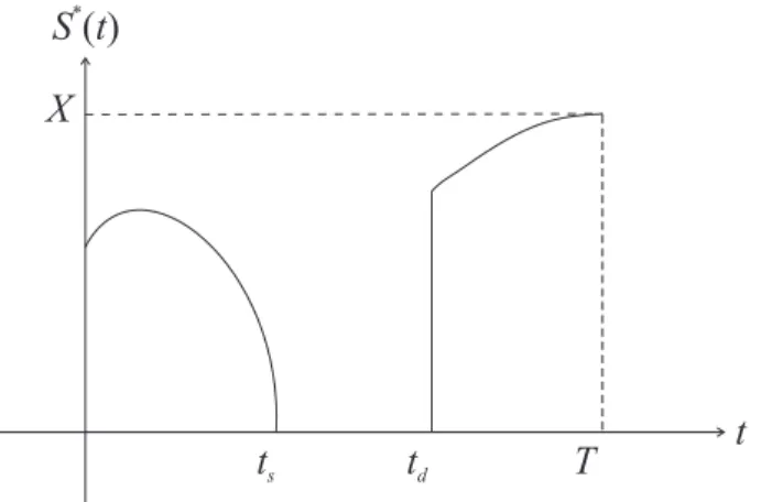
Cd(S, Te −t;X)≥ max{c(S, Te −t;X), c(S, td−t;X)}, t < td. (5.1.44) 5.1.6 One-dividend and multi-dividend American put options Consider an American put on an asset which pays out discrete dividends with certainty during the life of the option, the corresponding optimal exercise policy exhibits more complicated behaviors compared to its call counterpart. Within some short time period prior to a dividend payment date, the put holder may choose not to exercise at any asset price level due to the antic-ipation of the dividend payment. That is, the holder prefers to defer early exercise until immediately after an ex-dividend date in order to benefit from the receipt of the dividend by holding the asset through the dividend date. From the last dividend date to expiration, the optimal exercise boundary be-haves like that of an American put on a non-dividend payment asset, so the optimal exercise priceS∗(t) increases monotonically with increasing calendar timet. For times in between the dividend dates and before the first dividend date,S∗(t) may rise or fall with increasingtor even becomes zero (see Figs. 5.5 and 5.6). Due to the complicated nature of the optimal exercise policy, no analytic price formula exists for an American put on an asset paying discrete dividends.
One-dividend American put
First, we would like to consider the early exercise policy for the one-dividend American put model. Let the ex-dividend date betd, the expiration date beT and the dividend amount beD. Since the exercise policy att > tdis identical to that of American put on the same asset with zero dividend, it suffices to consider the exercise policy at time t before the ex-dividend date. Suppose the American put is exercised at timet, then the interest received fromtto td arising from time value of the strike price X is X[er(td−t)−1], whereris the riskless interest rate. When the interest is less than the discrete dividend, that is,X[er(td−t)−1]< D, the early exercise of the American put is never
optimal. This is because the benefit from the receipt of the dividend amount D by holding the asset through the dividend datetdis more attractive than the interest income gained. Therefore, there exists a period prior totd such that it is never optimal for the holder to exercise the one-dividend American put.
One observes that the interest income X[er(td−t)−1] depends ont
d−t, and its value increases whentd−t increases. There exists a critical valuets such that
Solving forts, we obtain ts=td− 1 rln 1 +D X . (5.1.45b) Over the interval [ts, td], it is never optimal to exercise the American put.
When t < ts, we have X[er(td−t)−1]> D. Under such condition, early
exercise may become optimal when the asset price is below certain critical value. The optimal exercise priceS∗(t) is governed by two offsetting effects, the time value of the strike and the discrete dividend. Whentis approaching ts, the dividend effect is more dominant so that the American put would be exercised only when it is deeper-in-the-money, that is, at a lower opti-mal exercise priceS∗(t). Whentis farther away fromts, the dividend effect diminishes so that the optimal exercise policy behaves more like usual Amer-ican put on a zero-dividend asset. In this case, S∗(t) assumes a lower value aststays farther fromts. As a result, the plot ofS∗(t) againsttresembles a humped shape curve for the time interval prior tots(see Fig. 5.5).
From Eq. (5.1.45b),ts is seen to increase with increasing r so that the interval of “no-exercise” [ts, td] shrinks with higher interest rate. Since the early exercise of an American put results in gain of time value of strike, a higher interest rate implies a higher opportunity cost of holding an in-the-money American put so that the propensity of early exercise increases.
Fig. 5.5The behaviors of the optimal exercise boundary
S∗(t) as a function oft for a one-dividend American put
option.
In summary, the optimal exercise boundary S∗(t) of the one-dividend
American put model exhibits the following behaviors (see Figure 5.5). (i) Whent < ts,S∗(t) first increases then decreases smoothly with
increas-ingtuntil it drops to the zero value atts.
(iii) Whent ∈(td, T], S∗(t) is a montonically increasing function of twith S∗(T) =X.
Multi-dividend American put
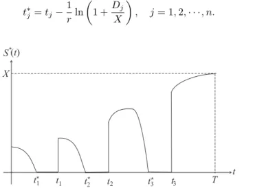
The analysis of the optimal exercise policy for the multi-dividend Ameri-can put model Ameri-can be performed in a similar manner. Suppose dividends of amount D1, D2, · · ·, Dn are paid on the ex-dividend dates t1, t2, · · ·, tn,
there is an interval [t∗j, tj] before the ex-dividend timetj, j= 1,2,· · ·, nsuch that it is never optimal to exercise the put prematurely. That is,S∗(t) = 0 fort∈[t∗j, tj], j= 1,2,· · ·, n., where the critical timet∗j is given by
t∗j =tj− 1 rln 1 +Dj X , j= 1,2,· · ·, n. (5.1.46)
Fig. 5.6 The characterization of the optimal exercise boundary S∗(t) as a function of the calendar time t
for a three-dividend American put option model. Ob-serve thatS∗(t) is monotonically increasing in (t
3, T) and S∗(T) =X. It stays at the zero value in [t∗
3, t3].
Further-more, S∗(t) can be increasing to some peak value then
decreasing as in (t2, t∗3), or simply decreasing
monotoni-cally as in (t1, t∗2).
Here, we follow the calendar time in the description of the optimal exercise boundary. At times falling within the intervals (tj−1, t∗j), j = 2,· · ·, nand
t≤t∗
1, the optimal exercise price S
∗(t) may first increase with time to some
peak value, then decreases and eventually drops to the zero value when the time reaches t∗
j. When the dividend is sufficently deep, S
∗(t) may decrease
monotonically throughout the interval (tj−1, t∗j) from some peak value to the
zero value. WhenDj increases further, it may be possible thatt∗j is less than
last time interval (tn, T], the optimal exercise price increases monotonically toX as expiration is approached.
The behaviors of the optimal exercise boundaryS∗(t) of a three-dividend American put model as a function of the calendar timetare depicted in Fig. 5.6. Meyer (2001) performed careful numerical studies on the optimal exercise policies of multi-dividend American put options. His results are consistent with the behaviors ofS∗(t) described above.
5.2 Analytic formulations of American option pricing
models
In this section, we consider two analytic formulations of American option pricing models, namely, the linear complementarity formulation and the for-mulation as an optimal stopping problem. First, we develop the variational inequalities that are satisfied by the American option price function, and from which we derive the linear complementarity formulation. Alternatively, the American option price can be seen to be the supremum of the discounted expectation of the exercise payoff among all possible stopping times. It can be shown rigorously that the solution to the optimal stopping formulation satisfies the linear complementarity formulation. From the theory of con-trolled diffusion process, we are able to derive the integral representation of an American price formula in terms of the optimal exercise boundary. We also show how to obtain the integral representation of the early exercise premium using the financial argument of delay exercise compensation. Using the fact that the optimal exercise price is the asset price at which one is indifferent between exercising or non-exercising, we deduce the integral equation for the optimal exercise price. This section is ended with the discussion of two types of American path dependent option models. We consider the pricing of the American barrier option and a special form of perpetual American lookback option coined with the name “Russian option”.
5.2.1 Linear complementarity formulation
The valuation of an American option can be formulated as a free boundary value problem, where the free boundary is the optimal exercise boundary which separates the continuation and stopping regions. When the asset price falls into the stopping region where the American call option should be ex-ercised optimally, we have
C(S, τ) =S−X, S≥S∗(τ). (5.2.1) The exercise payoff,C=S−X, does not satisfy the Black-Scholes equation since
∂ ∂τ − σ2 2S 2 ∂ 2 ∂S2 −(r−q)S ∂ ∂S +r (S−X) =qS−rX. (5.2.2a) FromS ≥S∗(τ)> S∗(0+) =Xmax 1,r q , we deduce thatqS−rX >0. We then deduce that in the stopping region, the call valueC(S, τ) observes the following inequality
∂C ∂τ − σ2 2S 2∂ 2C ∂S2 −(r−q)S ∂C ∂S +rC >0 for S≥S ∗ (τ). (5.2.2b) The above inequality can also be deduced from the following financial argument. LetΠdenote the value of the riskless hedging portfolio defined by
Π=C−∆Swhere∆= ∂C
∂S. (5.2.3a) We argue that optimal early exercise of the American call occurs when the rate of return from the riskless hedging portfolio is less than the riskless interest rate, that is,
dΠ < rΠ dt. (5.2.3b) By computingdΠ using Ito’s lemma, the above inequality can be shown to be equivalent to Ineq. (5.2.2b).
In the continuation region where the asset price S is less than the opti-mal exercise price S∗(τ), the American call value satisfies the Black-Scholes equation. We then conclude that
∂C ∂τ − σ2 2S 2∂ 2C ∂S2 −(r−q)S ∂C ∂S +rC≥0, S >0 andτ >0, (5.2.4) where equality holds when (S, τ) lies in the continuation region. On the other hand, the American call value is always above the intrinsic valueS−X when S < S∗(τ) and equal to the intrinsic value when S≥S∗(τ), that is,
C(S, τ)≥S−X, S >0 andτ >0. (5.2.5) In the above inequality, equality holds when (S, τ) lies in the stopping region. Since (S, τ) is either in the continuation region or stopping region, equality holds in one of the above pair of variational inequalities. We then deduce that
∂C ∂τ − σ2 2 S 2∂2C ∂S2 −(r−q)S ∂C ∂S +rC [C−(S−X)] = 0, (5.2.6) for all values ofS >0 andτ >0. To complete the formulation of the model, we have to include the terminal payoff condition in the model formulation
Inequalities (5.2.4–5) and Eq. (5.2.6) together with the auxiliary condition (5.2.7) constitute the linear complementarity formulation of the American call option pricing model (Dewynneet al., 1993).
From the above linear complementarity formulation, we can deduce the following two properties for the optimal exercise priceS∗(τ) of an American call.
1. It is the lowest asset price for which the American call value is equal to the exercise payoff.
2. It is the asset price at which one is indifferent between exercising and not exercising the American call.
Bunch and Johnson (2000) presents another interesting property ofS∗(τ). It is the lowest asset price at which the American call value does not depend on the time to expiry, that is,
∂C
∂τ = 0 at S=S ∗
(τ). (5.2.8) This agrees with the financial intuition that at the moment when it is optimal to exercise immediately, it does not matter how much time is left to maturity. A simple mathematical proof can be constructed as follows. On the optimal exercise boundaryS∗(τ), we have
C(S∗(τ), τ) =S∗(τ)−X. (5.2.9a) Differentiating both sides with respect toτ, we obtain
∂C ∂τ(S ∗ (τ), τ) +∂C ∂S(S ∗ (τ), τ)dS ∗(τ) dτ = dS∗(τ) ∂τ . (5.2.9b) Using the smooth pasting condition: ∂C
∂S(S ∗
(τ), τ) = 1, we then obtain the result in Eq. (5.2.8).
5.2.2 Optimal stopping problem
The pricing of an American option can also be formulated as anoptimal stop-ping problem. A stopstop-ping timet∗ can be considered as a function assuming value over an interval [0, T] such that the decision to “stop at timet∗” is de-termined by the information on the asset price pathSu,0≤u≤t∗. Consider an American put option, and suppose that it is exercised at timet∗, t∗< T, the payoff is max(X−St∗,0). The fair value of the put option with payoff at t∗ defined above is given by
Et[e−r(t∗−t)max(X−St∗,0)],
whereEtis the expectation under the risk neutral measure conditional on the filtrationFt. This is valid provided that t∗ is a stopping time, independent of whether it is deterministic or random.
Since the holder can exercise at any time during the life of the option, we deduce that the American put value is given by (Karatzas, 1988; Jacka, 1991; Myneni, 1992)
P(St, t) = sup t≤t∗≤T
Et[e−r(t∗−t)max(X−St∗,0)], (5.2.10)
where t is the calendar time and the supremum is taken over all possible stopping times. Recall thatP(St, t) always stays at or above the payoff and P(St, t) equals the payoff at the stopping time t∗. The above supremum is reached at the optimal stopping time (Krylov, 1980) so that
t∗= inf
u {t≤u≤T :P(Su, u) = max(X−Su,0)}, (5.2.11) the first time that the American put value drops to its payoff value.
We would like to verify that the solution to the linear complementarity formulation gives the American put value as stated in Eq. (5.2.10), where the optimal stopping time is determined by Eq. (5.2.11). We recall the renowed optional stopping theorem which states that if (Mt)t≥0 is a continuous
mar-tingale with respect to the filtration (Ft)t≥0, and ift∗1andt
∗
2are two stopping
times,t∗ 1< t ∗ 2, then E[Mt∗ 2|Ft ∗ 1] =Mt ∗ 1. (5.2.12)
For any stopping time t∗, t < t∗< T, we apply Ito’s formula to the solution P(St, t) of the linear complementarity formulation to obtain
e−rt∗P(St∗, t∗) =e−rtP(St, t) + Z t∗ t e−ru ∂ ∂t + σ2 2S 2 ∂2 ∂S2 + (r−q)S ∂ ∂S −r P(Su, u)du + Z t∗ t e−rσS∂P ∂S(Su, u)dZu. (5.2.13)
Now, the integrand of the first integral is non-positive as deduced from one of the variational inequalities [see Eq. (5.2.4)]. When we take the expectation of the martingle term in the second integral, the expectation value becomes zero by virtue of the optional sampling theorem. We then have
P(St, t)≥Et[e−r(t
∗
−t)P(S
t∗, t∗)]
=Et[e−r(t∗−t)max(X−St∗,0)]. (5.2.14)
Lastly, if we chooset∗as defined by Eq. (5.2.11), the above inequality becomes an equality, hence the result in Eq. (5.2.10).
5.2.3 Integral representation of the early exercise premium
From the theory of controlled diffusion process, the American put price is given by [a rigorous proof is presented in Krylov’s text (1980)]
P(St, t) =Et[e−r(T−t)max(X−ST,0)] + Z T t e−r(u−t)Eu(rX−qSu)1{Su<S∗(u)} du. (5.2.15) The first term represents the usual European put price while the second term represents the early exercise premium. Let ψ(Su;St) denote the transition density function ofSuconditional onSt. We may rewrite the above put price formula as follows P(St, t) =e−r(T−t) Z X 0 (X−ST)ψ(ST;St)dST + Z T t e−r(u−t) Z S∗(u) 0 (rX−qSu)ψ(Su;St)dSudu. (5.2.16) The early exercise premium is seen to be positive since
rX−qSu>0 as Su< S ∗
(u)<rX q .
We would like to provide an intuitive proof to the American put price formula by arguing that the early exercise premium can be interpreted as delay exercise compensation (Jamshidian, 1992).
Delay exercise compensation
In order that the American put option is kept alive for all values of asset price until expiration, the holder needs to be compensated by a continuous cash flow when the put should be exercised optimally. Within the time interval between uand u+duand suppose Su falls within the stopping region, the amount of compensation paid to the holder of the American put should be (rX−qSu)duin order that the holder agrees not to exercise even when it is optimal for him to do so. This is because the holder would earn interestrX du from the cash received and lose dividend qSudu from the short position of the asset if he were to choose to exercise his put. The discounted expectation for the above continuous cash flow compensation is given by
e−r(u−t) Z S∗(u)
0
(rX −qSu)ψ(Su;St)dSu.
The integration of the above discounted cash flow fromu=t tou=T gives the early exercise premium of the American put option, which is precisely the early exercise premium term in Eq. (5.2.16).
![Fig. 5.2 An American call on an asset paying continu- continu-ous dividend yield remains alive inside the continuation region {(S, τ ) : S ∈ [0, S ∗ (τ )), τ ∈ (0, T ]}](https://thumb-us.123doks.com/thumbv2/123dok_us/8938406.2380579/5.892.171.551.103.332/american-paying-continu-continu-dividend-remains-inside-continuation.webp)