Preemptive Rate-based Operator Scheduling
in a Data Stream Management System
∗Mohamed A. Sharaf, Panos K. Chrysanthis, Alexandros Labrinidis
Department of Computer Science
University of Pittsburgh
Pittsburgh, PA 15260, USA
{
msharaf, panos, labrinid
}
@cs.pitt.edu
Abstract
Data Stream Management Systems are being developed to process continuous queries over multiple data streams. These continuous queries are typically used for monitoring purposes where the detection of an event might trigger a sequence of actions or the execution of a set of specified tasks. Such events are identified by tuples produced by a query and hence, it is important to produce the available portions of a query result as early as possible.
A core element for improving the interactive perfor-mance of a continuous query is the operator scheduler. An operator scheduler is particularly important when the processing requirements and the productivity of different streams are highly skewed. The need for an operator sched-uler becomes even more crucial when tuples from different streams arrive asynchronously. To meet these needs, we are proposing a Preemptive Rate-based scheduling policy that handles the asynchronous nature of tuple arrival and the heterogeneity in the query plan. Experimental results show the significant improvements provided by our proposed pol-icy.
1
Introduction
A Data Stream Management System (DSMS) hosts ap-plications which rely on data that is continuously generated at remote sources. The DSMS is responsible for processing these data streams according to the applications’ require-ments and for streaming the relative results to each appli-cation. Such applications include monitoring a data net-work performance, fraud detection in telecommunication networks, monitoring the stock market, personalized Web
∗This work is supported in part by NSF ITR Medium Award
(ANI-0325353). The first author is supported in part by the Andrew Mellon Predoctoral Fellowship.
pages, and environmental monitoring via sensor networks. Recently, a number of prototype system have been de-veloped to accommodate the growing need for supporting the processing of data streams. Examples include: Aurora [3], STREAM [8], TelegraphCQ [5], and NiagaraCQ [6]. In these systems, continuous queries are registered at the DSMS and run continuously over the data streams. The ar-rival of new data triggers the execution of one or more con-tinuous queries. The objective of these systems is to provide data processing techniques that is tailored for the continu-ous nature of data handled by DSMSs.
The requirements of a DSMS are more demanding than those of a traditional DBMS for several reasons. In a tra-ditional DBMS, data is stored as relations and queries are posed on the stored relation. However, in a DSMS, data arrives in the form of continuous, unbounded, and pos-sibly bursty data streams. Moreover, a DSMS typically supports multiple long-running continuous queries over the data streams [10].
Continuous queries are typically used for monitoring purposes where the detection of an event might require trig-gering a sequence of action. This creates an interactive en-vironment where tuples produced by a query might activate the execution of specified tasks. In such an environment, it is important to optimize for producing the available portions of the result as early as possible rather than optimizing the computing of the entire result as in traditional database sys-tems. The timely generation of the initial results increases the probability of detecting events earlier.
The two main elements for improving the interactive per-formance of a continuous query are: 1) query optimizer, and 2) operator scheduler. The query optimizer decides the dependencies between the query operators, whereas the scheduler decides the order of execution of the query oper-ators. An operator scheduler is particularly important when a query is defined on multiple relations or streams.
underlying operating system. However, this approach over-looks chances for improvement that are possible by exploit-ing the available information about the query operators. The Rate-based scheduling presented in [12] exploits such infor-mation for improving the interactive query performance in traditional databases and in Web databases. Basically, it em-ploys a prioritizing scheme where the priority of an operator is defined in terms of its cost and selectivity.
Since the Rate-based policy was proposed for traditional database systems, it assumes priorities are static. However, in DSMSs, tuples continuously arrive at the system, some of which might correspond to a higher priority operator than the one currently executing. Thus, under Rate-based scheduling, high-priority operators might be blocked wait-ing for a low-priority one to complete its execution.
To alleviate this priority-inversion problem, in this pa-per, we propose a Preemptive Rate-based scheduling pol-icy. The intuition is that preemption enables the adjust-ment of a previous scheduling decision based on the current state that is determined by the arrival of new data. The idea of using preemption in scheduling query operators has already showed success in reducing the memory require-ments for processing bursty streams [1]. In this paper, we are also using the preemption mechanism but for improv-ing the interactive performance of queries with stateless op-erators. Our experimental evaluation shows the significant improvements provided by our proposed scheduling policy compared to the existing ones.
The rest of this paper is organized as follows. In Sec-tion 2 provides an overview of query processing, optimiza-tion and operator scheduling. Our model and scheduling polices are presented in Section 3. Section 4 describes our simulation testbed, and then in Section 5 we discuss our ex-periments and results. We conclude in Section 6.
2
DSMS Background
2.1
Continuous Queries
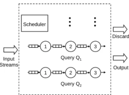
A Data stream management system (DSMS), as shown in Figure 1, is designed to handle the processing of multi-ple queries over multimulti-ple data streams. In such a system, users register continuous queries that execute as new data arrives. Data arrives in the form of continuous streams. The arrival of new data is similar to an insertion operation in tra-ditional database systems. A DSMS is typically connected to different data sources that generate streams at different rates. Moreover, a single query might receive its input from multiple streams (i.e., sources).
The query evaluation plan can be conceptualized as a data flow diagram [3, 1], which is a tree of nodes and edges, where the nodes are operators that process tuples and edges represent the flow of tuples from one operator to another
(Figure 2). An edge from operatorO1to operatorO2means that the output of operatorO1 is an input to operatorO2. The overall query cost is determined by the cost of each operatorCi and the selectivity of each operatorSi. Recall
that, an operator with selectivitySiproducesSituples after
processing one tuple forCitime units. Si is typically less
than or equal to 1 for simple operators like filters, but, it might be more than 1 for joins.
A single continuous query in a DSMS could be quite complicated and expensive, especially, if the query is han-dling data from multiple streams where tuples from each stream pass through several expensive operators. Moreover, the distribution of the processing costs of operators is typ-ically heterogeneous. That is, the costs for processing dif-ferent tuples from difdif-ferent streams could be highly skewed. For instance, a query plan might contain operators that per-form simple filtering on one data stream, whereas on an-other data stream complex operators might require join with stored relations or look-up indexes. Similarly, the selectiv-ity of different operators exhibit a skewed distribution. This heterogeneity makes it essential for using query processing techniques that provide an efficient execution plan for eval-uating the query.
2.2
Query Execution
In this work, we assume that each query is composed of only stateless operators. Queries with stateless operators is fairly common class of queries in data stream applications [1, 4]. Examples of stateless operators are scan, selection,
projection, and join with stored relations. Moreover, a
con-tinuous query over multiple streams typically contains spe-cial operators for merging different streams. Such an oper-ator is known as union [3], merge [7], or mux [9]. Studying queries with statefull operators (e.g., join over data streams) is part of our future work.
Every tuple that enters the system must pass through a unique sequence of operators, referred to as an operator
path [1]. The operator path corresponding to stream Str
might contain specialized operators that are only applicable on tuples fromStr, in addition to other operators that are applicable on more than one stream. A specialized operator is basically used for transforming an input tuple to match a pre-defined scheme, or to apply a certain filtering or map-ping for which the execution method depends on the corre-sponding data stream. For example, in Figure 2, operators forming the pathO1, O2, O3process tuples fromStream1,
O1 is applied only on tuples fromStream1, whileO2 is used to merge the intermediate result tuples fromStream1 andStream2. Finally,O3is used to project the final result tuples from both streams.
An operator receives its input tuples either directly from the input stream (e.g., operatorsO1andO4) or from
inter-Input Streams Output Discard Query Q2 1 2 3 Scheduler Query Q1 1 2 3
Figure 1. Data processing in DSMS
3 2 1 4 Stream2 Stream1 Output
Figure 2. Query plan over streams
mediate queues used to buffer the output of a predecessor operator (e.g., operatorsO2andO3). A tuple is processed until it is either produced at the output or discarded. A tuple is produced when it satisfies all the filters on the operator path. If a tuple does not satisfy a certain filter, it is immedi-ately discarded since it is not used by any other query.
The mechanism of invoking an operator depends on the underlying query execution architecture. In the single-thread architecture, all operators are running in the same thread and invoking an operator is equivalent to a procedure call. In the multiple-thread architecture, each operator runs in a separate thread and invoking an operator requires con-text switching between threads.
The scheduler is the system component responsible for invoking operators according to a special order of execu-tion. Specifically, it decides the following: 1) the order of query execution among the registered queries, and 2) the or-der of operator execution within a query. In this work, we are focusing on the latter problem of scheduling operators within a query. Specifically, we are interested into an opera-tor scheduling policy that improves interactive performance of continuous queries.
2.3
Operator Scheduling
Traditionally, query optimizers are cost-based in that they decide among alternative execution plans by minimiz-ing the query cost. That is, the estimated cost of evaluat-ing the query until the last result tuple appears [13]. How-ever, with the advent of the Internet, interactive query per-formance became an important criterion for evaluating the success of an online system. In such an interactive environ-ment, it is important to optimize for producing the available portions of the result as early as possible rather than opti-mizing the computing of the entire result. The same inter-active behavior is desirable in data stream systems for two main reasons. The first reason stems out of the nature of data stream processing; in DSMS data arrives continuously, hence, optimizing for producing the full result is obviously infeasible. The second reason depends on the timely re-quirements of the application supported by the DSMS. For
example, a user’s continuous query might be used to pro-cess readings gathered by sensor networks that monitor en-vironmental phenomena. In such a case, producing results as soon as they are available helps in accelerating the detec-tion of abnormal behaviors that require immediate acdetec-tions.
The two main elements for improving the interactive per-formance of a continuous query are: 1) query optimizer, and 2) operator scheduler. The query optimizer decides the de-pendencies between the query operators, whereas the sched-uler decides the order of execution of the query operators. The work in [13] proposed a rate-based query optimization technique that maximizes the output rate of query evalua-tion plans. This technique provides optimizaevalua-tion soluevalua-tions for the case when a query contains operators that joins two streams which have different data arrival rates. For all other cases, the plans generated by the rate-based optimization are the same as those generated using a cost-based opti-mizer. Moreover, for both of the optimization strategies, the way operators are scheduled and how the flow of data is controlled can lead to significantly different kinds of output behavior for the same generated query plan [12].
For an optimized query plan, Pipelined query execution is one technique that can improve the interactive perfor-mance of a query. In a pipelined execution model, the unit of execution is the processing of a single tuple on a single stream. In a fully pipelined execution plan, result tuples are delivered as soon as they are computed from the input tuples. Pipelining works only as long as operators are non-blocking, i.e., they do not stage the data without producing results for a long time. Filters are non-blocking operators by nature, whereas for blocking operators (e.g., join),
win-dowing is used to allow result streaming. However, for a
multiple-relation query (or multiple streams), pipelined ex-ecution does not specify the order of exex-ecution of operators on different streams. A scheduling policy is needed to de-termine which stream to process when more than one has available tuples.
The problem of operator scheduling has been the fo-cus of the work in [12]. It proposed a dynamic rate-based
pipeline scheduling policy that produces more results
response time. Aurora [3, 4] also uses a technique similar to the rate-based pipeline scheduling to minimize the average tuple latency.
2.4
Performance Metric
The performance of scheduling policies is typically mea-sured using the average response time. In traditional database systems, the response time of a query is defined as the amount of time from the time when the query is posed until the time when the last tuple in the result is produced.
However, in DSMSs, queries are continuous where a query is executed whenever new data arrives. That behavior is the opposite from traditional database systems; in tradi-tional systems, the response is due to the arrival of a query, whereas in data streams system, the response is triggered by the arrival of a tuple.
Hence, in DSMS, it is more appropriate to define the re-sponse time from the data perspective rather than the query perspective. Therefore, we will define the tuple response
time (or tuple latency) (Ri) for tupleias follows:
Definition 1 Ri =Di−Ai, whereAiis the tuple arrival
time andDi is the tuple departure time. Accordingly, the
average response time forN tuples is: N1 PNi Ri.
Notice that tuples that are filtered out during query process-ing do not contribute to this metric [11].
Example Let us illustrate that measuring the tuple
av-erage response time better reflects the interactive perfor-mance achieved by a scheduling policy. In Figure 2, as-sume that the costs of operators O1, O2, O3, O4 are 10, 10, 10, 40 units respectively. Further, assume that there is one tuple available for processing at each input stream. First, consider a scheduling policy that will activate opera-tors in the following order:O1, O2, O3to process the tuple fromStream1, thenO4, O2, O3to process the tuple from
Stream2. Such a policy will provide an average tuple re-sponse time of 60 units. An alternative scheduling might decide to schedule operator paths in the opposite order. That is, O4, O2, O3 to process the tuple from Stream2, then
O1, O2, O3 to process the tuple fromStream1. This al-ternative policy will provide an average response time of 75 units. Though both policies take the same time to complete execution (i.e., 90 units), they provide different response times. The improvement exhibited by the first policy is due to producing result tuples as early as possible which is the behavior desired for interactive performance.
3
Operator Scheduling Policies
In this section, we first discuss two operator scheduling policies, namely, Round Robin and Rate-based, which are
currently used in the prototype DSMSs. Then we will de-scribe our proposed preemptive version of the Rate-based scheduling policy.
3.1
Round Robin
Round Robin has been the policy used the most for pro-cessing sharing. It is simple and easy to implement. In Round Robin, each operator is assigned a time interval called quantum. At the end of the quantum, the processor is preempted and given to another operator.
By nature, Round Robin does not take advantage of the available parameters of operators (i.e., cost and selectivity). This is in contrast to using a priority-based scheduling pol-icy which assigns each operator a priority based on its pa-rameters. Ignoring this information makes Round Robin fall short in improving the interactive performance men-tioned above. For example, it is known that a priority-based policy like Shortest-Remaining-Processing-Time sig-nificantly outperforms Round Robin in improving the re-sponse time [2]. However, Round Robin does not need to recover from a wrong scheduling decision because simply there is no decision taken and preemption allows all opera-tors to execute sequentially.
3.2
Rate-based
The Rate-based scheduling policy was proposed for scheduling the execution of operators in a single query for the pipelined execution in traditional database systems [12]. Each operatorO has a value called the global output rate which is defined in terms of its ancestor operators. The out-put rate of an operatorOis basically the number of tuples produced per time unit by processing one tuple by the se-quence of operators starting atOall the way up to the out-put. Formally, the global output rate for operatorO1on the pathO1, O2, ..., Onis computed as:
S1×S2×...×Sn
C1+C2×S1+...+Cn×Sn−1×...×S1
(1) WhereCiandSiare the cost and the selectivity of operator Oi, respectively.
The priority of each operator is set to its global output rate. At each scheduling point, the operator with the highest priority among all operators with non-empty input queues is the one scheduled for execution. In this policy, the sched-uler is triggered (i.e., scheduling point is reached) when an operator finishes processing an input tuple. The new opera-tor scheduled for execution can be the ancesopera-tor of the previ-ously scheduled operator since it already has a higher prior-ity. This higher priority is due to the increased probability of producing the tuple and/or the decrease in the remaining
execution time required to produce the tuple. Alternatively, the new scheduled operator might be the leaf node of a dif-ferent operator path for which a corresponding tuple has ar-rived at the scheduling point or during the execution of the previous operator.
The intuition underlying this policy is to produce the ini-tial output tuples as fast as possible. This is achieved by giving higher priority to operator paths that are productive and inexpensive or, in other words, select the operator path with the minimum latency for producing one tuple.
3.3
Preemptive Rate-Based
In data stream systems, tuples continuously arrive at the system; query execution is triggered by the arrival of new tuples. That is different from traditional database systems, for which the Rate-based policy was originally proposed. The problem with the continuous arrival of tuples is that a newly arriving tuple might correspond to a higher-priority path. Toward this, we are proposing a preemptive version of the rate-based policy so that a higher-priority path can be selected if such a path become available.
In this preemptive version, if operatorOi is already
se-lected for execution then the next scheduling point could be triggered whileOi is still in progress. That is, scheduling
occurs in the following cases:
1. Operator Oi finishes processing: This case is the
same as in the non-preemptive version where a new scheduling decision is made every time an operator fin-ishes executing.
2. The arrival of a new tuple at a leaf operatorOj: In
this case, the priority of operatorOj is compared to
the current priority ofOiwhere the latter is computed
given the intervalδit already spent processing the cur-rent tuple. In other words, the global output rate ofOi
is recomputed by replacingCi withCi −δin
Equa-tion 1. Then the operator with the highest priority is scheduled for execution.
The intuition in using preemption is to be able to adjust the scheduling decision based on the current situation that is determined by the arrival of new data. In the absence of preemption, not only an inexpensive operator might have to wait until the currently relatively expensive operator fin-ishes execution, but also, a productive operator might have to wait until a less productive operator finishes execution. Using preemption is particularly important when the dis-tribution of operators costs and/or selectivities is highly skewed. In such a case, the priority assigned to operators span a long range of values. This is in contrast when the operators parameters are homogeneous, then the priority values assigned to operators are fairly close and blocking a
Preemptive Non-Preemptive
Pipelined PRB RB, FIFO
Non-Pipelined RR Train Processing
Table 1. Classification of Scheduling Policies
high priority operator until finishing the execution of a less priority one will have a little impact on the performance.
It is worth mentioning that ifOiis preempted due to the
arrival of new a tuple atOj, thenOiwill not resume
execu-tion again until all the operators on the operator path starting atOj finish execution. This is because of the following: 1)
the priority ofOidoes not increase while executingOj, and
2) the priority of all the operators on the path fromOjto the
output is higher than the current priority ofOi. The latter
observation follows from the fact thatOj has a higher
pri-ority thanOiand that an ancestor ofOjwill have a higher
priority than Oj as explained above. Thus, a preempted
operator is not considered again until higher priority oper-ators finish execution. This shows the limited increase in scheduling overhead introduced by allowing preemption.
3.4
Discussion
Above, we described three policies for scheduling query operators, namely, Round Robin (RR), Rate-based (RB), and our proposed Preemptive Rate-based (PRB). In the next section, we provide a performance evaluation of these poli-cies in addition to the First-In-First-Out (FIFO) scheduling policy. FIFO is implemented following the pipelined execu-tion model where a tuple is completely processed along its operator path before the processing of a new tuple starts. However, in the presence of ready tuples from multiple streams, we use the tuple’ timestamp as a tie-breaker to de-cide the order, where a tuple’s timestamp is the time when the tuple entered the system.
Table 1 shows a classification of the four policies accord-ing to two features, namely, preemption and pipelinaccord-ing. The table also includes the Train processing mechanism used by Aurora for controlling the flow of tuples along a path [4]. A train is a sequence of tuples that are executed as a batch within an operator that is selected for execution using a rate-based policy. The goal of tuple train processing is to mini-mize the low-level overheads in a single-thread query exe-cution architecture. In the case where the length of the train is one tuple, then train processing is fully pipelined and is similar to the Rated-based policy. Hence, we will only use the Rate-based policy as a representative of the two tech-niques.
It is worth mentioning that the proposed Preemptive Rate-based policy could be used for scheduling operators from multiple queries in order to improve the overall sys-tem response time. However, with multiple queries fairness
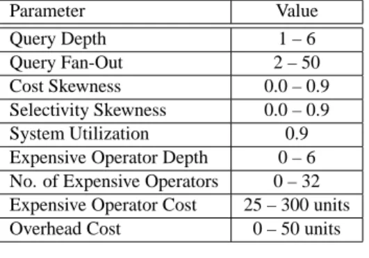
Parameter Value Query Depth 1 – 6 Query Fan-Out 2 – 50 Cost Skewness 0.0 – 0.9 Selectivity Skewness 0.0 – 0.9 System Utilization 0.9 Expensive Operator Depth 0 – 6 No. of Expensive Operators 0 – 32 Expensive Operator Cost 25 – 300 units Overhead Cost 0 – 50 units
Table 2. Simulation Parameters
in scheduling is an issue to be considered. Such a problem is the focus of our future work.
4
Evaluation Testbed
In our experimental evaluation, we have used the aver-age tuple response time metric from Section 2 to compare the query performance provided by the scheduling policies mentioned above. Accordingly, we simulated the execution of a continuous query as in [4] where the query is speci-fied by two parameters: depth and fan-out. The depth of the query specifies the number of levels in the query tree and the fan-out specifies the number of children for each operator.
The costs and selectivities of the query operators are generated according to a Zipf distribution which is speci-fied using the Zipf parameter. Setting the Zipf parameter to zero results in a uniform distribution, whereas increasing the value of the Zipf parameter increases the skewness of the generated values.
Each leaf operator is attached to a data stream where tu-ples arrive according to a Poisson distribution. The mean inter-arrival time for the Poisson distribution is set accord-ing to the simulated system utilization (or load). For a uti-lization of 1.0, the inter-arrival time is equal to the time re-quired to complete the query execution, whereas for lower utilizations, the mean inter-arrival time is increased propor-tionally. All the results reported here are at a utilization of 0.9 and stream length of 10K tuples.
Finally, we use additional parameters to control the het-erogeneity in the query plan, namely, Expensive Operator
Depth, No. of Expensive Operators, and Expensive Opera-tor Cost. Finally, we use the Overhead Cost parameter for
calculating the overheads incurred by the different policies. The usage of the above parameters is explained along with the experiments in the next section. Table 2 summarizes all our simulation parameters.
5
Experiments
5.1
Skewness in Operators’ Costs
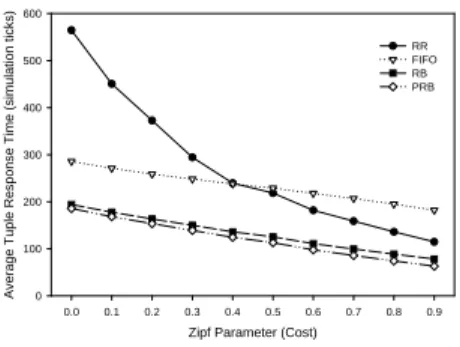
In this experiment we set the query depth to 1 and the fan-out to 50. This is equivalent to a query that performs projection and/or filtering on 50 data streams then merge them together. The costs of the operators are generated in the range 1–100 with skewness 0.9 toward the inexpensive operators. The selectivity for all operator is set to 1.
Figure 3 shows the average tuple response time provided by the Round Robin (RR), First-In-First-Out (FIFO), Rate-based (RB) and the Preemptive Rated-Rate-based (PRB) policies. The figure shows that, in general, the average response time decreases by increasing the skewness of operators’ costs. For instance, the minimum response time is achieved at a Zipf parameter of value 0.9 where most of the operators are inexpensive. In the case of Zipf parameter of value 0.0, the operators’ costs are uniformly distributed which results in higher response time.
The figure also shows that as the degree of skewness in-creases, RR outperforms FIFO. Recall that Both RR and FIFO ignore the operators’ characteristics (i.e., cost and se-lectivity), however, the figure shows that at high skewness, preemption can improve the performance. This observation is emphasized by comparing the response times provided by the Preemptive Rate-based (PRB) and the non-preemptive version (i.e., RB) where PRB always outperforms RB as well as RR and FIFO.
This improvement is better illustrated in Figure 4. Fig-ure 4 shows the reduction in average response time provided by PRB compared to RB. The figure shows that the im-provement increases by increasing the skewness. For ex-ample, the reduction is only 5% when the Zipf parameter is equal to 0.0 and it increases to 20% when the Zipf param-eter is equal to 0.9. The increase in improvement is due to the increased heterogeneity in the query plan. In a plan with a highly skewed operators’ costs, using RB might result in a case where a newly arriving tuple might have to wait for the currently executing tuple though the latter might have a relatively very high execution cost. PRB avoids this by allowing the preemption of the expensive operator.
5.2
Skewness in Operators’ Selectivities
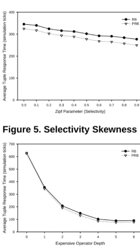
The setting for this experiment is similar to the previous one, however, we are changing the skewness of selectivity while setting the cost of all operators to 100 units. From now on, we will exclude RR and FIFO from the comparison due to their high response time as illustrated in Figure 3.
Operators take selectivities in the range 0.01 – 1.0 which are generated using Zipf. The skewness of the Zipf param-eter is toward the low-selectivity operators. In this setting,
Zipf Parameter (Cost) 0.0 0.1 0.2 0.3 0.4 0.5 0.6 0.7 0.8 0.9 A v e rage T up le R e s pon s e T im e (s im u la ti on ti c k s ) 0 100 200 300 400 500 600 RR FIFO RB PRB
Figure 3. Cost Skewness
Zipf Parameter (Cost)
0.0 0.1 0.2 0.3 0.4 0.5 0.6 0.7 0.8 0.9 R e d u c ti o n in A v e ra g e R e s po n s e T im e 0% 5% 10% 15% 20% 25% PRB Figure 4. Reductions by PRB vs. RB
at a high value for the Zipf parameter, most of the streams will have low priority while very few will have a relatively high priority.
Figures 5 and 6 show the same behavior illustrated in the previous experiment. That is, PRB always outperforms RB and that the significance of reduction in response time in-creases by increasing the skewness. Hence, in order to avoid repetition, the remaining of this section will only report on experiments where we are varying the cost distribution.
5.3
Skewness’ Position
In the previous experiments, we changed the skewness of the cost and selectivity distributions, yet, we had no control on the position of the skewness in the query plan. Figure 7 shows another experiment where we are controlling the lo-cation of skewness.
Specifically, we generated a query tree of depth 6 and fan-out 2 where we set the cost for all operators uniformly between 1 and 10 units. Then we introduced one expensive
operator of cost 100. This expensive operator is located on
the left-most operator path in the tree. However, the depth of the expensive operator is defined by a parameter
Expen-sive Operator Depth. In the case where expenExpen-sive operator
depth is equal to 6, the operator at the bottom-left corner of the tree is the most expensive, accordingly, the left operator path of the tree is the only expensive path. Decreasing the depth of the expensive operator is equivalent to increasing the number of expensive path. In the case where expensive operator depth is equal to 0, the root of the tree is the most expensive operator, hence, all the query path are relatively expensive. Figure 7 shows that generally, the average re-sponse time decreases by increasing the expensive operator depth. This decrease is due to a decrease in the number of expensive paths as mentioned above.
In Figure 8 we are illustrating the reduction in response time provided by PRB compared to RB. Notice that the im-provement increases by increasing the expensive operator depth (i.e., decreasing the number of expensive paths). This behavior is due to increasing the skewness in the query tree where preemption is needed. The improvement reaches a
maximum at expensive operator depth value of 4 (i.e., 4 ex-pensive operators paths), then it starts decreasing for values of 5 and 6. At a value of 5, there are only 2 expensive paths in the tree and at a value of 6, there is only one ex-pensive path. The low number of exex-pensive paths decreases the chances of an expensive operator to be running at the ar-rival time of a new tuple that corresponds to an inexpensive operator.
5.4
Skewness’ Amount
To further study the effect of skewness’ location and amount, we conducted another experiment that is shown in Figure 9. The settings for this experiment is similar to the previous one, however, the location and the number of the expensive operators are set differently. In this experiment, we are varying the number of expensive operators between 1 and 32. Further, the expensive operators are all located at depth 6 (i.e., the leaf nodes). Hence, the number of ex-pensive paths is always equal to the number of exex-pensive operators.
Figure 9 shows the same behavior demonstrated in Fig-ure 7. That is, the average response time increases by in-creasing the number of expensive operator path. Moreover, Figure 10 emphasizes the impact of the amount of skewness on the degree of improvement. For instance, at very low number of expensive operators/paths there are less chances of priority conflict between current and new tuples. As the number of expensive paths increases, the chances of a pri-ority conflict increases. Further increase in the number of expensive paths brings the tree close to homogeneity, hence, less chances of priority conflict.
5.5
Skewness’ Magnitude
Figure 11 shows the results of an experiment where we are changing the cost of the expensive operator. Specifi-cally, there is one expensive operator in the query plan lo-cated at depth 4. The cost of this expensive operator takes the values between 25 and 300 time units. The figure shows that PRB outperforms RB. Moreover, it shows that RR can
Zipf Parameter (Selectivity) 0.0 0.1 0.2 0.3 0.4 0.5 0.6 0.7 0.8 0.9 A v e rage T up le R e s pon s e T im e (s im u la ti on ti c k s ) 0 100 200 300 400 RB PRB
Figure 5. Selectivity Skewness
Zipf Parameter (Selectivity)
0.0 0.1 0.2 0.3 0.4 0.5 0.6 0.7 0.8 0.9 R edu c ti on in A v e rage R e s pon s e T im e 0% 2% 4% 6% 8% 10% 12% PRB Figure 6. Reductions by PRB vs. RB
Expensive Operator Depth
0 1 2 3 4 5 6 A v e ra g e T up le R e s p on s e T im e (s im u la ti o n ti cks ) 0 100 200 300 400 500 600 700 RB PRB
Figure 7. Location of Skewness
Expensive Operator Depth
0 1 2 3 4 5 6 7 R e d u c ti o n in A v e ra g e R e s p on s e T im e 0% 2% 4% 6% 8% 10% 12% 14% 16% 18% PRB Figure 8. Reductions by PRB vs. RB
also outperform RB when the cost of the expensive oper-ator is set relatively high. This is because scheduling the expensive operator for execution might result in the arrival of many tuples that belong to inexpensive operator paths. In such a case, RR and PRB allow preempting the currently ex-ecuting expensive operator and proceed with exex-ecuting the less expensive one to produce more result tuples, whereas RB will wait for the expensive operator to finish then it will make new scheduling decisions. The higher the cost of the operator, the longer the RB will wait, and the more the in-crease in the average response time.
5.6
Scheduling Policy Overhead
Figure 12 shows the results of our last experiment where we are measuring the overhead of each scheduling policy. As mentioned earlier, the overheads depend on the under-lying query execution architecture. However, instead of as-suming a certain architecture, we counted the number of transitions between states during query execution. Transi-tions happen in the following cases: 1) invoking an operator, 2) preempting an operator, and 3) invoking the scheduler.
RR incurs the overheads of all three transitions: at the end of each quantum an operator is preempted and the scheduler is invoked to find the next operator in the cycle with available tuples which is then invoked for execution. In RB, the first and the third transitions take place, where when an operator finishes execution, the scheduler is invoked and the operator with the highest priority is executed. PRB in-curs the same overheads as RB in addition to the overheads
due to enabling preemption. Specifically, the scheduler is invoked with the arrival of every new tuple which might re-sult in preempting the currently executing operator.
In Figure 12 we assigned the same cost to each type of the transitions mentioned above. We call this parameter
overhead cost and its takes the values between 0 and 60.
The value of the overhead cost together with the number of transitions determine the total overhead incurred by a cer-tain scheduling policy. In Figure 12, we measured the re-sponse time at the point where the expensive operator cost is 300 as in Figure 11. The figure shows the increase in re-sponse time with the increase in overhead cost. Moreover, it shows that RR outperforms RB only when the overhead cost is 0. As the overhead costs becomes 1, the performance of RR is highly unacceptable (note that in this figure, we use logarithmic scale for the Y-axis as opposed to the previous figures). This high overhead incurred by RR is due to the continuous preemption of operators. The rate of preemption is determined by the quantum length. In these experiments we assumed a quantum of length 1 time unit. Higher values for the quantum will show lower overhead, yet, significantly high compared to RB and PRB. The figure also shows that PRB scheduling outperforms the non-preemptive RB for values of overhead cost up to 50 time units. However, a value of 50 is an unrealistic overestimation of the overhead cost, since this represents an overhead equal to≃16.6%of the expensive operator cost. Recall that an expensive oper-ator might require looking up indexes or performing a join with a stored relation, in either cases, the cost of that opera-tor should be orders of magnitude the overhead cost.
Number of Expensive Operators 0 4 8 12 16 20 24 28 32 36 A v e ra g e T up le R e s p on s e T im e (s im u la ti o n ti cks ) 0 50 100 150 200 250 300 350 RB PRB
Figure 9. Amount of Skewness
Number of Expensive Operators
0 4 8 12 16 20 24 28 32 36 R edu c ti on in A v e rage R e s pon s e T im e 4% 6% 8% 10% 12% 14% 16% 18% 20% PRB Figure 10. Reductions by PRB vs. RB
Expensive Operator Cost
0 50 100 150 200 250 300 350 A v e rage T up le R e s pon s e T im e (s im u la ti on ti c k s ) 0 50 100 150 200 250 RR RB PRB
Figure 11. Magnitude of Skewness
Overhead Cost 0 10 20 30 40 50 60 70 A v e rage T up le R e s pon s e T im e (l og s c a le ) 1e+1 1e+2 1e+3 1e+4 1e+5 1e+6 RR RB PRB
Figure 12. Impact of Overheads
6
Conclusions
The rapid growth of DSMSs introduces more challenges to the database systems research. Challenges are mainly due to the continuous nature of data and the timely requirements of the continuous queries. This new environment requires rethinking the existing data processing techniques for effi-cient design of DSMSs. In this paper, we addressed one of those techniques, namely, query processing. Specifically, we focused on the operator scheduling component of query processing. The paper makes the following contributions:
1. It emphasizes the importance of the rate-based pipelined scheduling policies for scheduling query op-erators over multiple heterogeneous data streams. 2. It points out the importance of preemption in query
op-erator scheduling which is particularly crucial to suit the asynchronous nature of tuple arrival.
3. It proposes the Preemptive Rate-based scheduling pol-icy which combines the advantages of pipelined exe-cution, rate-based scheduling, and preemption. Our extensive experimental evaluation shows the signif-icant improvements provided by our proposed Preemptive Rated-based policy. Currently, we are studying the problem of scheduling multiple queries over data streams.
References
[1] B. Babcock, S. Babu, M. Datar, and R. Motwani. Chain: Op-erator scheduling for memory minimization in data stream systems. In ACM SIGMOD Conf., 2003.
[2] N. Bansal and M. Harchol-Balter. Analysis of SRPT scheduling: Investigating unfairness. In ACM SIGMETRICS
Conf., 2001.
[3] D. Carney et al. Monitoring streams: A new class of data management applications. In VLDB Conf., 2002.
[4] D. Carney et al. Operator scheduling in a data stream man-ager. In VLDB Conf., 2003.
[5] S. Chandrasekaran et al. TelegraphCQ: Continuous dataflow processing for an uncertain world. In CIDR Conf., 2003. [6] J. Chen, D. J. DeWitt, F. Tian, and Y. Wang. NiagaraCQ: A
scalable continuous query system for internet databases. In
ACM SIGMOD Conf., 2000.
[7] C. Cranor, T. Johnson, O. Spataschek, and V. Shkapenyuk. Gigascope: A stream database for network applications. In
ACM SIGMOD Conf., 2003.
[8] R. Motwani et al. Query processing, resource management, and approximation in a data stream management system. In
CIDR Conf., 2003.
[9] M. Sullivan. A stream database manager for network traffic analysis. In VLDB Conf., 1996.
[10] D. B. Terry, D. Goldberg, D. Nichols, and B. M. Oki. Contin-uous queries over append-only databases. In ACM SIGMOD
Conf., 1992.
[11] F. Tian and D. J. DeWitt. Tuple routing strategies for dis-tributed eddies. In VLDB Conf., 2003.
[12] T. Urhan and M. J. Franklin. Dynamic pipeline schedul-ing for improvschedul-ing interactive query performance. In VLDB
Conf., 2001.
[13] S. D. Viglas and J. F. Naughton. Rate-based query optimiza-tion for streaming informaoptimiza-tion sources. In ACM SIGMOD