Policy Research Working Paper
6351
How Much International Variation in Child
Height Can Sanitation Explain?
Dean Spears
The World Bank
Sustainable Development Network
Water and Sanitation Program
February 2013
WPS6351
Public Disclosure Authorized
Public Disclosure Authorized
Public Disclosure Authorized
Abstract
The Policy Research Working Paper Series disseminates the findings of work in progress to encourage the exchange of ideas about development issues. An objective of the series is to get the findings out quickly, even if the presentations are less than fully polished. The papers carry the names of the authors and should be cited accordingly. The findings, interpretations, and conclusions expressed in this paper are entirely those of the authors. They do not necessarily represent the views of the International Bank for Reconstruction and Development/World Bank and its affiliated organizations, or those of the Executive Directors of the World Bank or the governments they represent.
Policy Research Working Paper 6351
Physical height is an important economic variable reflecting health and human capital. Puzzlingly, however, differences in average height across developing countries are not well explained by differences in wealth. In particular, children in India are shorter, on average, than children in Africa who are poorer, on average, a paradox called “the Asian enigma” which has received much attention from economists. This paper provides the first documentation of a quantitatively important gradient between child height and sanitation that can statistically explain a large fraction of international height differences. This association between sanitation and
This paper is a product of the Water and Sanitation Program, Sustainable Development Network. It is part of a larger effort by the World Bank to provide open access to its research and make a contribution to development policy discussions around the world. Policy Research Working Papers are also posted on the Web at http://econ.worldbank.org. The author may be contacted at [email protected].
human capital is robustly stable, even after accounting for other heterogeneity, such as in GDP. The author applies three complementary empirical strategies to identify the association between sanitation and child height: level regressions across 140 country-years in 65 developing countries; within-country analysis of differences over time within Indian districts; and econometric decomposition of the India-Africa height differences in child-level data. Open defecation, which is exceptionally widespread in India, can account for much or all of the excess stunting in India.
How much international variation in child height can
sanitation explain?
Dean Spears
∗First circulated: 10 December 2012
This version: 17 January 2013
Abstract
Physical height is an important economic variable reflecting health and human capital. Puzzlingly, however, differences in average height across developing countries are not well explained by differences in wealth. In particular, children in India are shorter, on average, than children in Africa who are poorer, on average, a paradox called “the Asian enigma” which has received much attention from economists. This paper provides the first documentation of a quantitatively important gradient between child height and sanitation that can statistically explain a large fraction of interna-tional height differences. This association between sanitation and human capital is robustly stable, even after accounting for other heterogeneity, such as in GDP. I apply three complementary empirical strategies to identify the association between sanitation and child height: country-level regressions across 140 country-years in 65 developing countries; within-country analysis of differences over time within Indian districts; and econometric decomposition of the India-Africa height difference in child-level data. Open defecation, which is exceptionally widespread in India, can account for much or all of the excess stunting in India.
∗Princeton University. Wallace Hall. Princeton, NJ 08540. [email protected]. I am grateful for helpful suggestions from Luis Andres, Robert Chambers, Juan Costain, Jean Dr`eze, Marianne Fay, Ariel Fiszbein, John Newman, Doug Miller; from seminar participants at LBSNAA, Princeton, and the World Bank and WSP; and especially from Anne Case, Diane Coffey, Angus Deaton, Michael Geruso, and Jeff Hammer. Errors and interpretations are my own. Portions of this paper have previously circulated as “Sanitation and open defecation explain international variation in childrens height: Evidence from 140 na-tionally representative household surveys” and “What does the NFHS-3 (DHS) tell us about rural sanitation externalities?,” both of which this working paper supersedes.
1
Introduction
Physical height is a topic of expanding interest to economists (Steckel, 2009), in large part because it is an important correlate of human capital and health and is a predictor of eco-nomic productivity (Currie, 2009). Despite this attention, an important puzzle persists: international differences in height across present day developing countries are not well ex-plained by differences in economic well-being (Deaton, 2007). In particular, people in India are shorter, on average, than people in Africa, despite the fact that Indians are also richer, on average, a fact that has been labeled the “Asian enigma” (Ramalingaswami et al., 1996). One candidate explanation which has received relatively little attention in economists’ recent investigations of the puzzle of Indian stunting (e.g. Deaton, 2007; Tarozzi, 2008; Jayachandran and Pande, 2012; Panagariya, 2012) is sanitation. Medical research documents that chronic childhood environmental exposure to fecal germs can be an important cause of stunting (Humphrey, 2009). Sanitation coverage is exceptionally poor in India, where over half of households defecate openly without using a toilet or latrine, a much larger fraction than in other countries with similar income.
According to joint UNICEF and WHO (2012) estimates for 2010, 15 percent of people in the world, and 19 percent of people in developing countries, openly defecate without using any toilet or latrine. The primary contribution of this paper is to document that much of the variation in child height among developing countries can be explained by differences in rates of open defecation. Sanitation robustly explains variation in stunting, even after accounting for GDP and other dimensions of heterogeneous economic development. Other recent papers, concentrating on internal validity, have demonstrated the existence of a causal effect of sanitation on child height (Spears, 2012a; Hammer and Spears, 2012); in contrast, this paper assesses the statistical global importance of sanitation quantitatively, using descriptive regressions and econometric decomposition techniques. In particular, differences in open defecation are sufficient to statistically explain much or all of the difference in average height
between Indian and African children. These results suggest that open defecation is a policy priority of first-order importance.
This paper makes several contribution to the literature. First, to my knowledge, it offers the first documentation of a quantitatively important cross-country gradient between sanitation and child human capital. Although the association between income and health has been widely studied within and across developing countries, the importance of sanitation has received much less attention. Moreover, I show that sanitation predicts child height even conditional on income. Controlling for GDP, the difference between Nigeria’s 26 percent open defecation rate and India’s 55 percent is associated with an increase in child height approximately equivalent to quadrupling GDP per capita.
Second, this paper documents an interaction between sanitation and population density, consistent with a mechanism in which open defecation harms human capital through exposure to environmental germs. The number of people defecating openly per square kilometer linearly explains 65 percent of international variation in child height. This finding clarifies the policy case for sanitation as a public good. Third, it contributes to a resolution of the puzzle of the “Asian enigma” of Indian stunting, which has received much recent attention from economists. Finally, the conclusions offer a reminder that height, often refereed to as an indicator of “malnutrition,” broadly reflects early-life net nutrition, including losses due to disease.
Three sections of the paper contribute complementary analyses of the relationship be-tween height and open defecation, each focusing on a different dimension of heterogeneity. Section 2 studies country-year average sanitation and child heights; here, each observation is a collapsed DHS survey. Open defecation is particularly harmful to children’s health where population density is high, creating a special risk of stunting in India. Section 3 compares children within one country, introducing district fixed effects to repeated cross-section data constructed out of two rounds of India’s National Family and Health Survey, in order to study differences within districts over time. Section 4 considers whether the
India-Africa height gap can be explained by heterogeneity in village-level open defecation rates, using individual-level data on child heights and decomposition analysis in the spirit of Oaxaca-Blinder. Reweighting Indian data to match the sanitation of an African sample counterfactually increases the height of Indian children by more than the India-Africa gap. All three approaches find a similar and quantitatively important association between height and sanitation. Finally, a concluding section 5 considers whether estimates of of the asso-ciation between height and sanitation in this paper and from the literature are sufficient to account for the India-Africa gap.
1.1
Open defecation causes stunting
A growing literature in economics documents that physical height has its origins in early life health (e.g. Case and Paxson, 2008), especially in poor countries where environmental threats to health are more important than they are in rich countries, relative to genetics (Martorell et al., 1977; Spears, 2012b). Two existing literatures indicate that early-life expo-sure to fecal germs in the environment reduces children’s subsequent height. First, medical and epidemiological literatures have documented the mechanisms linking open defecation to poor health and early life human capital accumulation.1 Humphrey (2009) documents that chronic but subclinical “environmental enteropathy” – a disorder caused by repeated fecal contamination which increases the small intestine’s permeability to pathogens while reducing nutrient absorption – could cause malnutrition, stunting, and cognitive deficits, even without necessarily manifesting as diarrhea (see also Petri et al., 2008; Mondal et al., 2011). Relat-edly, Checkley et al. (2008) use detailed longitudinal data to study an association between childhood diarrhea and subsequent height.
Second, recent econometric studies find an effect of a government sanitation program in
1Perhaps the recent paper most complementary to this one is Fink et al.’s (2011) regression of an indicator
for child stunting on variables including sanitation in 172 pooled DHS surveys. However, one key difference is that they focus on within-country height-sanitation correlations: all regressions include DHS survey fixed effects for country-years.
rural India. From 1999 until its replacement with a new program in 2012, the Indian central government operated a “flagship” rural sanitation program called the Total Sanitation Cam-paign (TSC). Averaging over implementation heterogeneity throughout rural India, Spears (2012a) finds that the TSC reduced infant mortality and increased children’s height, on aver-age. In a follow-up study, Spears and Lamba (2012) find that early life exposure to improved rural sanitation due to the TSC additionally caused an increase in cognitive achievement at age six. Similarly, Hammer and Spears (2012) report a randomized field experiment in Ma-harashtra, in which children living in villages randomly assigned to a treatment group that received sanitation motivation and subsidized latrine construction grew taller than children in control villages. Section 5.1 considers the estimates of these causally well-identified studies in the context of this paper’s results.
1.2
Open defecation is common in India
Of the 1.1 billion people who defecate openly, nearly 60 percent live in India, which means they make up more than half of the population of India. These large numbers are roughly corroborated by the Indian government’s 2011 census, which found that 53.1 percent of all Indian households – and 69.3 percent of rural households – “usually” do not use any kind of toilet or latrine. In the 2005-6 National Family Health Survey, India’s version of the DHS, 55.3 percent of all Indian households reported defecating openly, a number which rose to 74 percent among rural households.
These statistics are striking for several reasons. First, open defecation is much more common in India than it is in many countries in Africa where, on average, poorer people live. UNICEF and the WHO estimate that in 2010, 25 percent of people in sub-Saharan Africa openly defecated. In the largest three sub-Saharan countries – Nigeria, Ethiopia, and the Democratic Republic of the Congo – in their most recent DHS surveys, 31.1, 38.3, and 12.1 percent of households report defecating openly.
de-clined in India over the past two decades, not even during the rapid growth period since the early 1990s. In the DHS, where 55.3 percent of Indian households defecated openly in 2005-06, 63.7 did in the earlier 1998 survey round, and 69.7 did in 1992. This is particularly true for poor people: the joint UNICEF and WHO report concludes that “the poorest 40 percent of the population in Southern Asia have barely benefited from improvements in sanitation.” In 2010, 86 percent of the poorest quintile of South Asians defecated openly.
Therefore, it is already well-known that open defecation is bad for children’s health; that early-life disease leads to lasting stunting; and that open defecation is exceptionally widespread in India. The contribution of this paper is to quantitatively assess the importance of the link among these facts. The results indicate that sanitation is a statistically important predictor of differences in the height of children in developing countries and can explain differences of interest to economists and of significance to human development.
2
Evidence from country means: 140 DHS surveys
Across countries, observed in different years, how much of the variation in child height is explained by variation in open defecation? This section uses 140 DHS surveys, each collapsed into a single observation, to show that sanitation alone explains more than half of the variation across country-years.
The analysis proceeds in several steps. First, section 2.2 documents that, across country means, height is associated with open defecation, with little change after controlling for GDP. Next, section 2.2.1 uses country fixed effects and replication on sub-samples of world regions to show that no geographic or genetic differences are responsible for the result. Then, section 2.2.2 verifies that other dimensions of infrastructure or well-being do not similarly predict child height. Section 2.2.3 observes that children would be more exposed to fecal pathogens where population is more dense, and finds that open defecation interacts with population density. Section 2.2.4 documents that the association between height and open defecation is
steeper among older children, consistent with an unfolding effect of accumulating exposure. Finally, section 2.3 considers the average height difference between children in South Asian and Sub-Saharan African countries, and shows that much of this gap is accounted for by sanitation.
2.1
Data
All data used in this paper are publicly available free of charge on the internet. Demographic and Health Surveys (DHS) are large, nationally representative surveys conducted in poor and middle-income countries. DHS surveys are collected and organized to be internationally comparable. In some countries, several rounds of DHS data have been collected; in others only one or two. I use every DHS survey which recorded household sanitation and measured child height.2 This creates a maximum sample of 140 country-years and 65 countries, ranging
in frequency from 26 countries that appear in the survey once to 10 that appear in four separate DHS surveys. The earliest survey in the dataset was collected in Pakistan in 1990; the most recent are from 2010.
I match data from other sources to the collapsed DHS surveys. GDP per capita and population are taken from the Penn World Tables. “Polity” and “Democracy” scores of democratization are taken from the Polity IV database. A measure of calorie availability produced by the World Food Program is used in some specifications. All other variables are from DHS surveys.
Using these data, the basic regression I estimate is
heightcy =βopen def ecationcy+αc+γy+Xcyθ+εcy, (1)
where observations are collapsed DHS surveys,cindexes countries, andyindexes years. Open defecation is a fraction from 0 to 1 of the population reporting open defecation without using
2I use published summary statistics available online at www.measuredhs.com. DHS surveys do not include
a toilet or latrine.3 Height is the average height of children under 5 or children under 3, used
in separate regressions. As robustness checks, results are replicated with country fixed effects
αc, year fixed effectsγy, and time-varying controlsXcy, including the log of GDP per capita,
all of which are added separately in stages. Standard errors are clustered by 65 countries.
2.2
Regression results
Figure 1 depicts the main result of this section: a negative association between open defeca-tion and child height is visible across country years both for children under 3 and children under 5. Regression lines are plotted with and without weighting by country population. The three largest circles are India’s National Family and Health Surveys (only one large cir-cle appears in panel (b) because only the 2005 survey measured height of children up to age 5). Average height in India is, indeed, low. However, the fact that the Indian observations are on the regression line – and not special outliers – is an initial suggestion that sanitation might help resolve the “Asian enigma” of Indian height.
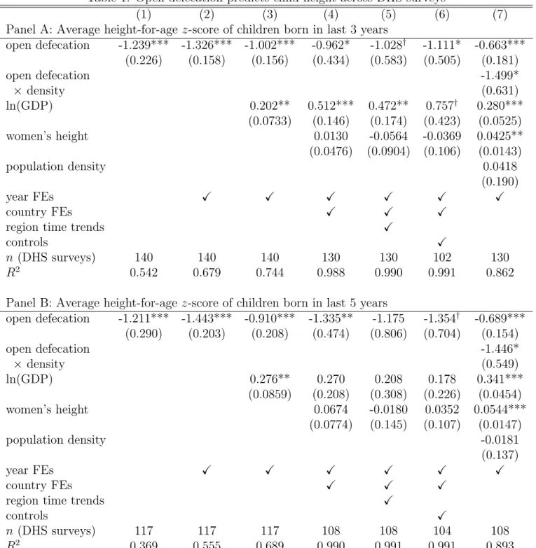
Table 1 reports estimates of regression 1 and will be referenced throughout this section of the paper. The main estimate of a linear decrease in height of 1.24 standard deviations associated with changing the fraction openly defecating from 0 to 1 is qualitatively similar to Spears’s (2012a) estimates of 1.15 to 1.59, where effects of sanitation are identified using heterogeneity in the implementation of an Indian government program. In column 1, san-itation alone linearly explains 54 percent of the country-year variation of children’s height in DHS surveys. Because sanitation and height are both improving over time, column 2 adds year fixed effects; the point estimates slightly increase and standard errors decrease, suggesting that the result is not an artifact of time trends.
Does the significance of open defecation merely reflect general economic development? Column 3 adds a control for GDP per capita; the coefficient on sanitation remains similar,
3For example, in India’s NFHS-3, the survey asks “What kind of toilet facility do members of your
household usually use,” with the relevant answer “No facility/uses open space or field.” This importantly distinguishes latrine use from latrine ownership.
which is consistent with Deaton’s (2007) observation that income does not explain cross-country height differences.4 This is reflected in panel (a) of figure 2, which plots the residuals
after regressing height of children under 3 years old on the log of GDP against the residuals after regressing open defecation on the log of GDP. The association remains, and the R2
is similar: sanitation linearly explains 54.2 percent of variation in child height, and the sanitation residual explains 53.9 percent of the variation in the height residual.
Panel (b) of figure 2 adds average height and exposure to open defecation in wealth subsets of India’s 2005 DHS to the basic plot of country mean height and sanitation. Included in published DHS data is a classification of households into wealth quintiles based on asset ownership. Average height of children within these groups is plotted against the rate of open defecation among all households in the primary sampling unit where they live, that is, the local open defecation to which they are exposed. Additionally, I follow Tarozzi (2008) in identifying an elite top 2.5 percent of the Indian population: children who live in urban homes with flush toilets that they do not share with other households; whose mothers are literate and have been to secondary school; and whose families have electricity, a radio, a refrigerator, and a motorcycle or car. Even these relatively rich children are shorter than healthy norms; this is expected, because 7 percent of the households living near even these rich children defecate openly. Indeed, the graph shows that their stunted height is approximately what would be predicted given the open defecation in their environment. More broadly, the association between height and sanitation among these wealth groups is close to the the international trend computed from country means. Exposure to nearby open defecation linearly explains 99.5 percent of the variation in child height across the five asset
4GDP per capita statistically significantly interacts with open defecation to predict height: height\
cy =
−1.42−1.18open def ecationcy+ 0.14 ln (GDP)cy−0.59open def ecationcy×ln (GDP)cy, where open
defe-cation and GDP are demeaned, the coefficients on open defedefe-cation and the interaction are statistically sig-nificant at the 0.01 level, and GDP is statistically sigsig-nificant at the 0.05 level. Thus, the slope on ln(GDP) would be 0.36 with no open defecation, but only 0.038 at India’s 2005 level of open defecation, consistent with the low apparent effect of recent Indian economic growth on stunting. Although it is difficult to interpret this result causally, one possibility is that private health inputs such as food do less to promote child height in a very threatening disease environment; I thank Angus Deaton for this suggestion.
quintiles.
2.2.1 A geographic or genetic artifact?
Perhaps people who live in certain countries or regions tend to be tall or short, and this is coincidentally correlated with open defecation. Is the result driven by certain countries or regions, or fixed differences such as genetics?
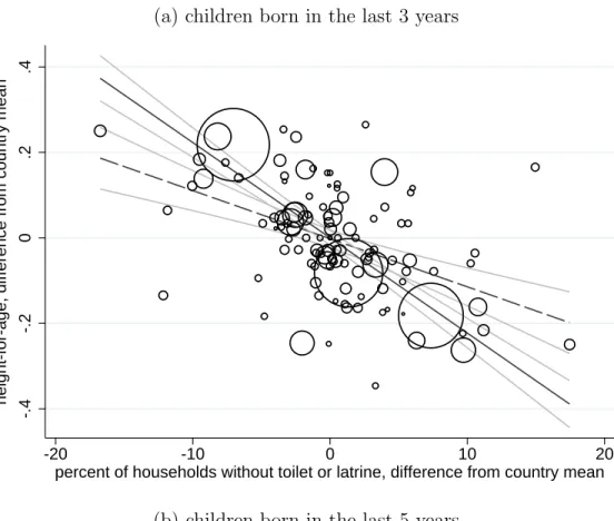
Figure 3 presents initial evidence against this possibility. The sample is restricted to countries with more than one DHS observation, and country means across collapsed DHS surveys are subtracted from the height and sanitation survey averages. The figure plots the difference in a country-year’s height from that country’s mean across DHS surveys against the difference in sanitation. The slope is similar to the undifferenced plot. Moreover, panel (b) continues to demonstrate an association despite not including any data from India.
Returning to table 1, column 4 adds country fixed effects. A control is also added for the average height of mothers of measured children; this is in anticipation of a possibility observed by Deaton and Dr`eze (2009) and considered in more depth in section 4.3 that Indian stunting is not caused by current nutritional deprivation or sanitary conditions, but is instead an effect of historical conditions that stunted the growth of women who are now mothers, restricting children’s uterine growth. DHS surveys are categorized into six global regions;5 column 5
adds six region-specific linear time trendsP
rδryeary, to rule out that the effect is driven by
spurious changes in specific parts of the world. Neither of these additions importantly change the estimate of the coefficient, although adding so many controls increases the standard errors.
Table 2 further confirms that no one region is responsible for the results. The association between height and sanitation is replicated in regressions that omit each of the six world regions in turn. The coefficient near 1 notably remains when South Asian observations are
5The regions are sub-Saharan Africa, South Asia, the Middle East & North Africa, Central Asia, East &
omitted, again suggesting that the result is not merely reflecting India.
2.2.2 A statistical coincidence?: Omitted and placebo variables
Across rich and poor places, good conditions are often found together, and problems are often found in places with other problems. Would any measure of infrastructure, governance, or welfare be as correlated with height as is sanitation?
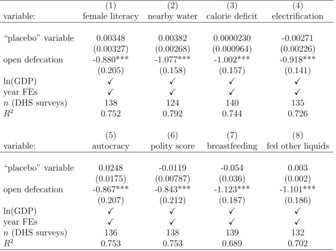
Column 6 of table 1 adds time-varying controls. These include female literacy, which is an important predictor of child welfare, and accessibility of water supply, all also from the DHS.6 Development outcomes are often attributed to good “institutions;” the set of controls
includes the polity and autocracy scores from the Polity IV database. With these controls added, the association between height and sanitation is essentially unchanged.7
Table 3 isolates each of these alternative independent variables in turn. None of these “placebo” predictors matter for child height, conditional on sanitation and and GDP.8 In particular, conditional on sanitation and GDP, child height is not associated with other types of infrastructure (electrification, water), governance (a democratic polity, autocracy), female literacy, or nutritional measures such as food availability, the breastfeeding rate,9 or
the fraction of infants who are fed “other liquids” beyond breastmilk in the last 24 hours.
6Despite the frequency of undifferentiated references to “water and sanitation,” improving water supply
and reducing open defecation have very different effects on child health and other outcomes and should not be conflated (Black and Fawcett, 2008).
7If controls for the fraction of infants ever breastfed, the fraction of infants breastfed within the first day,
and the fraction of infants fed “other liquids” in the past 24 hours are further added as measures of the quality of infant nutrition, the coefficient on open defecation in panel A with all controls becomeslarger in absolute value, -1.59, with a standard error of 0.82. This is not statistically significantly larger than the other estimates.
8Some of them do predict child height in a less thoroughly controlled specification. For example, in the
first column, if GDP is removed the coefficient on female literacy almost doubles and becomes statistically significant at the 0.1 level.
9Breastfeeding is an especially important variable because India has high levels of open defecation, short
children, and poor breastfeeding. In a regression with open defecation, country fixed effects, log of GDP, the fraction of children ever breastfed, and the fraction of children breastfed on the first day, neither breast-feeding variable is statistically significant (tof 0.23 and 0.6 respectively), but open defecation has a similar coefficient of -0.849, statistically significant at the two-sided 0.1 level (n = 139). If open defecators per square kilometer is used in place of the open defecation fraction, again it is statistically significant (t=−6) and the breastfeeding variables are not.
2.2.3 Mechanism: Interaction with population density
If open defecation is, indeed, stunting children’s growth by causing chronic enteric infection, then height outcomes should be consistent with this mechanism. In particular, children who are more likely to be exposed to other people’s fecal pathogens due to higher population density should suffer from larger effects of open defecation. For example, Ali et al. (2002) show that higher population density is associated with greater cholera risk in a rural area of Bangladesh, and Spears (2012a) finds a greater effect of India’s Total Sanitation Campaign in districts with higher population density.
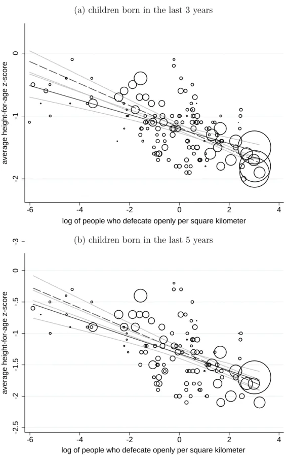
To test this conjecture, I construct a crude measure of “open defecators per square kilometer”: the product of population density per square kilometer times the fraction of people reporting open defecation. Figure 4 reveals that this measure of exposure to fecal pathogens (in logs, due to wide variation in population density) visibly predicts average child height. The regression in panel (a) of the figure explains 65 percent of variation in child height. Notably, India occupies the bottom-right corner of the graph, with high rates of open defecation and very high population density.
Does population density add predictive power beyond open defecation alone? The final column of table 1 adds an interaction between open defecation and population density. The interaction term is statistically significant, and the interaction and population density are jointly significant with, an F2,63 statistic of 4.5 (p= 0.0149) in column (a) andF2,57statistic
of 4.5 (p= 0.0155) in column (b).
A further implication of this mechanism is that open defecation will have a steeper association with child height in urban places than in rural places (Bateman and Smith, 1991; Bateman et al., 1993). Table 4 investigates this using two additional collapsed datasets, one containing only the urban observations in each DHS survey and one containing only the rural observations. Although GDP per capita is not available for urban and rural parts of countries, urban and rural women’s height controls can similarly be computed from the
DHS. In all cases, the urban coefficient on open defecation is greater than the whole-country coefficient and the rural coefficient is smaller. Hausman tests (reported under the open defecation coefficients in columns 5 through 7) verify that urban coefficients are larger than rural coefficients from the corresponding specifications.
2.2.4 Mechanism: A gradient that steepens with age
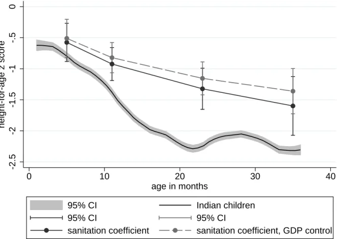
Height-for-age z scores are computed by age-in-months so that, in principle, the heights of children of different ages can be pooled and compared. If international reference charts were genetically or otherwise inappropriate for some countries, we might expect a consistent gap across children of different ages, analogous to a country fixed effect. However, stunting in India and elsewhere develops over time: children’s mean z-scores fall relative to the norm until about 24 months of age, where they flatten out. This is consistent with early-life health deprivation causing a steepening “gradient” between health and economic status, more steeply negatively sloped as children age (Case et al., 2002). If the association between height and sanitation were indeed the unfolding result of accumulating exposure to fecal pathogens, then it is plausible that the association would become steeper over the first two years of life, at a rate that flattens out.
Figure 5 plots the coefficients from estimating the basic equation 1 separately for collapsed means of children in four age groups: 0-5 months, 6-11 months, 12-23 months, and 24-35 months. Thus, as in the rest of this section of the paper, each coefficient is computed in a regression with 140 country means, but now these height means only include children in subsets of the age range. The independent variable – country-wide open defecation – is the same in each regression.
Two conclusions are visible in the figure. First, the gradient indeed steepens in age, at a rate that flattens. Second, the mean height of Indian children in the 2005 NFHS-3 is plotted for reference. The curve has a similar shape to the age pattern of the coefficients. This suggests that a fixed exposure to open defecation could be scaled into a similar shape as the
Indian height deficit by an increasing association between sanitation and height.
2.3
The gap between South Asia and sub-Saharan Africa
Although people in South Asia are, on average, richer than people in sub-Saharan Africa, children in South Asia are shorter, on average, and open defecation is much more common there. How much of the South Asia-Africa gap can sanitation statistically explain, at the level of country averages?
Table 5 estimates regressions in the form of equation 1, with the sample restricted to countries in South Asia and sub-Saharan Africa and with an indicator variable added for data from South Asia. Of the 140 DHS surveys in figure 1, 11 are from South Asia and 78 are from sub-Saharan Africa. In these data, children in South Asia are, on average, about one-third of a height-for-age standard deviation shorter.10
How do further controls change the estimate of this South Asia indicator? Merely lin-early controlling for open defecation reduces the gap by 30 percent from 0.360 to 0.253. Controlling, instead, for the number of people openly defecating per square kilometer (the product of population density and the open defecation rate, column 4) reduces the coefficient by 83 percent to 0.061. Column 5 verifies that this result is not merely a misleading effect of population density, controlling for which increases the gap.
Pairs of columns 6-7 and 8-9 demonstrate the statistical robustness of the explanatory power of the density of open defecation. After controlling for the log of GDP per capita, adding a further control for open defecators per square kilometer explains 73 percent of the (larger) remaining gap. The density of open defecation reduces by 92 percent the height
10 Jayachandran and Pande (2012), using individual-level DHS data from Africa and South Asia, suggest
that first-born South Asian children are taller than first-born African children. The country-level data studied here, however, show no similar reversal. If country means are computed using only first-born children, I find that South Asian children are 0.22 standard deviations shorter (s.e.= 0.05), a reduction but not an elimination of the 0.36 gap in table 5. In this sample of country means of first-borns, the gap falls to 0.15 with a control for open defecation and to 0.08 with a control for open defecation per square kilometer. In the full sample of country-level means of first-borns, analogously to column 1 of table 1, moving from an open defecation rate of 0 to 1 is linearly associated with a decline in height for age of 1.11 standard deviations.
gap after controlling for both log of GDP and year fixed effects. Sanitation initially appears to explain much of the Africa-South Asia gap in child height. Section 4.4 considers the decomposition of this difference in more detail, using child-level height data.
3
Evidence from differences within Indian districts
How much of the change over time in Indian children’s height is accounted for by the increase over time in sanitation coverage? One challenge to answering this question well is that, unfortunately, improvements in sanitation in India have been slow. As an illustration, in its 2005-6 DHS, 55.3 percent of Indian households reported open defecation, and the mean child was 1.9 standard deviations below the reference mean; this combination is almost identical to neighboring Pakistan’s in its 1990-1 DHS 15 years earlier, when 53.1 percent of households did not use a toilet or latrine and the mean height for age was 2 standard deviations below the mean. This section studies change over time within India by constructing a panel of districts out of India’s 1992-3 and 1998-9 DHS surveys.
3.1
Data and empirical strategy
The National Family and Health Surveys (NFHS) are India’s implementation of DHS surveys. This section analyzes a district-level panel constructed out of the NFHS-1 and NFHS-2.11
Districts are political subdivisions of states. Some districts merged or split between survey rounds, so households in the survey are matched to a constructed “district” that may be a coarser partition than actual district boundaries. In particular, a primary sampling unit (PSU) is assigned to a constructed district such that all splits and merges are assigned to the coarser partition, creating the finest partition such that each PSU is in the same constructed district as all PSUs which would have shared a district with it in either period. Thus if there were two districts A and B in the first round, which split before the second round into A0,
B0, and C (a new district containing part of A and of B), then all of A, B, A0, B0, and C
would be a single constructed district, although splits this complicated are rare.12
The empirical strategy of this section is to compare the heights of rural children under 3 years old in the NFHS rounds 1 and 2, using district fixed effects.13 In particular, I
regress child height on the fraction of households reporting open defecation at two levels of aggregation: districts and villages (or more precisely, rural primary sampling units). Because open defecation has negative externalities on other households, it is necessary to test for effects of community-wide sanitation coverage, rather than simply comparing households that do and do not have latrines; section 4.1 considers the econometric implications of these negative externalities in more detail.
Therefore, the regression specification is:
heightidvt=β1opendefecationdtd +β2opendefecationvdvt+αd+γt+Xidvtθ+Aidvtϑ+εidvt, (2)
where i indexes individual children, d are districts, v are villages (rural PSUs), and t are survey rounds 1 and 2. The dependent variable,heightidvtis the height of childiin standard
deviations, scaled according to the WHO 2006 reference chart. As recommended by the WHO, outliers are excluded with z-scores less than -6 or greater than 6. The independent variablesopendefecationddtandopendefecationvdvtare computed fractions 0 to 1 of households reporting open defecation in the child’s district and village, respectively. Fixed effectsαdand
γt are included for districts and survey rounds. The vector Aidvt is a set of 72 indicators for
age-in-month by sex, one for each month of age for boys and for girls.14 ControlsX
idvt are at
the household or child level: electrification, water supply, household size, indictors for being
12The NFHS was not constructed to reach all districts, so households are only included in the sample if
they are members of districts that appear in both survey rounds, to permit district fixed effects.
13Although district fixed effects are used, the NFHS did not survey the same villages in the two survey
rounds; thus there remains an important cross-sectional component to the heterogeneity studied.
14Panagariya (2012) has recently argued that height-for-agezscore reference charts are inappropriate for
Indian children; because age-in-months-by-sex is the level of disaggregation used to create height-for-age scores, these controls fully and flexibly account for any deviation between the mean height of Indian children and the reference charts.
Hindu or Muslim, a full set of birth order indicators interacted with the relationship of the child’s mother to the head of the household, twinship indicators, and month-of-birth indica-tors.15 Results are presented with and without controls and fixed effects to verify robustness.
The mean PSU studied here contains 10 children under 3 used in these regressions.
3.2
Regression results
Table 6 presents results from estimations of equation 2, with simple OLS in Panel A and district fixed effects in Panel B. Districts which saw greater differences in sanitation also present greater differences in child height.
District-level open defecation rates do not statistically significantly predict child height once village-level open defecation is included, which plausibly suggests that villages are much nearer than districts (which are much larger than villages) to capturing the geographic extent of sanitation externalities. Village-level open defecation predicts child height with or without district fixed effects and with or without individual controls.16 The coefficient on village open
defecation is smallest in absolute value with fixed effects and controls,17 although it is not
statistically significantly different from the other estimates; this could reflect the well-known attenuating bias of fixed effects, if much of the important variation in sanitation that is causing variation in height has been captured by other controls, leaving noise remaining.18
15If the survey rounds were conducted in different places in different times of year, different children would
be under 36 months old. Month of birth is correlated with early-life human capital inputs (cf. Doblhammer and Vaupel, 2001, about developed countries).
16If, instead of omitting observations with height-for-agez-score beyond±6, a cut-off of±10 is used, then
results are very similar. For example, the coefficient in column 1 of panel A becomes -0.768 (0.222); the smallest coefficient in absolute value, column 3 in Panel B, becomes -0.292 (0.138). If the log of height in centimeters is used as the dependent variable instead of thez score, moving from 0 percent to 100 percent open defecation is associated with an approximately 2 percent decrease in height (t ≈ 4, analogously to column 2 of panel B).
17Would any village-level (instead of household-level) asset or indicator of well-being have the same effect
as sanitation? Adding village electrification and water averages to the most controlled regression, column 3 of panel B, changes the point estimate on open defecation only slightly, from -0.35 to -0.33 (s.e.= 0.12); these two village level variables have t-statistics of 1.15 and -0.59, respectively, with a joint F-statistic of 0.73.
18For readers concerned about this possibility, regressing height on village-level open defecation with no
district or time fixed effects produces an estimate of -0.700 (t ≈4.5) and of -0.0501 (t≈4.8) with all the non-fixed-effect controls.
Consistency of fixed effects estimates, which subtract level differences across groups, depends on a properly linear specification. Column 4 demonstrates that a quadratic term for village-level open defecation is not statistically significant, and indeed changes signs with and without district fixed effects. Potential non-linear relationships between village sanitation coverage and child height will be considered in more detail in 4.1.2.
4
Evidence from pooled Indian and African surveys
Do differences in village-level sanitation coverage explain the difference in height between rural children in India and in sub-Saharan Africa? If so, is this just a spurious reflection of other correlated variables? This section addresses these questions using pooled child-level data from the rural parts of nine DHS surveys: India’s 2005-6 NFHS-3 and eight surveys from Africa in the 2000s.19 In particular, the DHS surveys nearest 2005 (and balanced before and
after) were selected from the five largest African countries available;20the included countries
account for 46 percent of the 2012 population of sub-Sahara Africa.
The argument of this section proceeds in several stages, building to a statistical decom-position of the India-Africa height difference, in the sense of Oaxaca-Blinder. First, section 4.1 verifies an association between village-level sanitation and height within the two regions. In particular, this section assesses the linearity of the relationship (assumed by some decom-position techniques), and notes that a village-level effect implies the presence of negative externalities. Then, section 4.2 considers a paradox implied by Deaton’s (2007) finding that height is not strongly associated with GDP: the within-region association between open defe-cation and well-being has a different slope from the across-region association. Next, section
19Here I again follow the WHO recommendation of dropping observations with height-for-age z-scores
more than 6 standard deviations from the mean.
20This excludes South Africa, where height has not been measured in a DHS survey. Beyond this data
availability constraint, this exclusion may be appropriate due to South Africa’s unique history and demog-raphy; its exceptionally high sanitation coverage (11.6 percent open defecation in 1998) would make it a positive outlier even in the African sample. The eight African DHS surveys used are: DRC 2007, Ethiopia 2000 and 2005, Kenya 2005 and 2008, Nigeria 2003 and 2008, and Tanzania 2004. DHS sampling weights are used throughout.
4.3 considers an alternative account of stunting in India: could it be a mere effect of short mothers causing restricted fetal growth, reflecting historical conditions and not a healthy environment that might exist today? Finally, section 4.4 proceeds with the decomposition, applying linear and non-parametric approaches to explain the India-Africa gap.
4.1
Effects of village sanitation: A negative externality
As a first step towards explaining the height difference between Indian and African children, this section verifies that village-level open defecation predicts children’s height within each region. As in section 3, I use household-level DHS data to find the fraction of households in a PSU reporting open defecation, which I treat as an estimate of village-level open defecation.
Thus, separately for each region r Africa and India, I estimate:
heightivcr = β1opendefecationvvcr+β3opendefecation2vcr+β3opendefecationiivcr+
αc+Xivcrθ+Aivcrϑ+εivcr,
(3)
where iindexes individual children under 5, v are villages (rural PSUs),care country-years (DHS surveys) in Africa and states in India, and r are regions (India or Africa). The de-pendent variable, heightivcr is the height of child i in standard deviations, scaled according
to the WHO 2006 reference chart. The independent variable open defecationvvcr is the com-puted fraction 0 to 1 of households reporting open defecation in the child’s village (again, implemented as rural primary sampling unit), with a quadratic term included in some spec-ifications. Household-level open defecationopendefecationiivcr is an indicator, 0 or 1, for the child’s household. Including both household and village-level open defecation tests whether one household’s open defecation involves negative externalities for other households.21 In
other words, is it only a household’s own sanitation that matters, or do other households’ sanitation matter, even controlling for one’s own?
21G¨unther and Fink’s (2010) working paper version of Fink et al. (2011) conducts a similar analysis,
Fixed effects αc are included for some specifications. As before, the vector Aivcr is a set
of 72 indicators for age-in-month by sex, one for each month of age for boys and for girls. Finally, Xivcr is a vector of child or household level controls: indicators for household dirt
floor; access to piped water; electrification; and ownership of a TV, bicycle, motorcycle, and clean cooking fuel; and the child’s mother’s literacy, knowledge of oral rehydration, age at first birth, count of children ever born, and relationship to the head of the household. These controls help ensure that any correlation between height and open defecation is unlikely to reflect mere wealth differences.
4.1.1 Regression results
Figure 6 plots, separately for the African and Indian samples, the local polynomial regres-sions of child height on village open defecation, separating households that do and do not defecate openly. The figures make clear the distinct private and social benefits of sanitation. The private benefit is the vertical distance between the two lines; thus, in an average Indian village, children in households that do not openly defecate are about half of a standard devi-ation taller than children in households that do. The social benefit – a negative externality on other households – is visible in the downward slope of the regression lines: children living in villages with less open defecation overall are taller, on average. Of course, some fraction of these correlations also reflects omitted variable bias. The dashed vertical lines show that open defecation is much more common in the Indian than in the African data. Moreover, children in households that do not practice open defecation are shorter in Africa than in India at all levels of village open defecation.
Table 7 verifies the statistical significance of these results and estimates regression equa-tion 3. In both samples, there is a clear associaequa-tion between child height and village-level sanitation. Especially in the Indian sample, the estimate changes little when controls are added. The coefficient on household-level sanitation is less robust: in the Indian sample it becomes much smaller when household and child controls are added, and in the African
sample it loses statistical significance.
4.1.2 Linear effects on height?
So far, this paper has largely studied linear regression. A non-linear relationship between sanitation and height could be important for two reasons: first, fixed effects regression could be inconsistent; and second, a linear Blinder-Oaxaca decomposition could be inappropriate. Returning to figure 6, the relationship between sanitation and height appears approximately linear in the Indian data, but may not be among openly-defecating households in the African data.
Non-linearity can be tested by adding a quadratic term. Already, in table 6, a quadratic term was not statistically significant in the first two Indian DHS surveys. Panel A finds again that, in the Indian NFHS-3, there is no evidence for a quadratic term. In contrast, Panel B does find a quadratic term in the African sample. In light of the evidence for the importance of open defecation per square kilometer presented in section 2.2.3, one possible explanation for this negative quadratic term is that population density is relatively low in these African countries, so open defecation is not as important for health until there is more of it; unfortunately, geographic data such as population density is not generally available at the DHS PSU level.
Many sanitation policy-makers claim that there is a discontinuous increase in health when open defecation is fully eliminated. This belief was importantly popularized by Sanan and Moulik (2007), who assert that “public health outcomes can be achieved only when the entire community adopts improved sanitation behavior, the area is is 100 percent open defecation free, and excreta safely and hygienically confined” (4).22 Whether the relationship between
sanitation and health is linear or another shape, it is clear from figure 6 that there is no
22This conclusion was based on a study by an organization called Knowledge Links in three villages of
Himachal Pradesh, which found a “prevalence of diarrhea” of 26 percent in a village where 95 percent of households used toilets, and of 7 percent in a village where 100 percent used toilets. Also see Shuval et al. (1981).
discontinuity at zero open defecation. Moreover, the statistically significant quadratic terms in Panel B of table 6 are negative, which suggests that, if anything, effects of village-level sanitation on height are smaller near perfect coverage in that sample.
4.2
A paradox: International differences in well-being
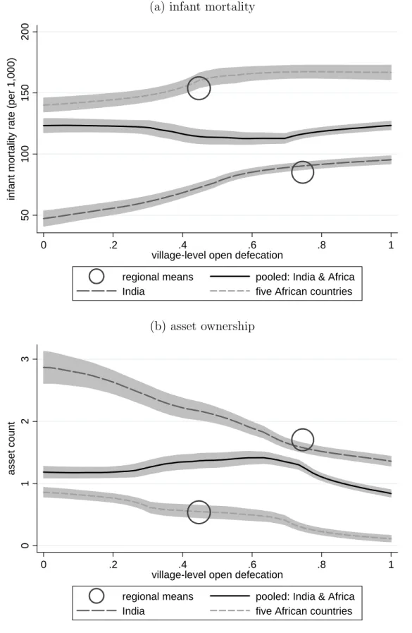
Deaton (2007) finds that international differences in height are not well explained by differ-ences in GDP or infant mortality. How could this be, given that poor sanitation increases infant mortality (Spears, 2012a), and richer people are more likely to have toilets or latrines? Figure 7 suggests that this puzzle is an example of Simpson’s Paradox: within separate subsets of a larger sample, the relationship between two variables can be very different from the relationship between the two variables in the larger, pooled sample.23 In particular, the relationship in the pooled data also depends upon the relationship among group means. Consider a large dataset partitioned into subsets indexeds∈S. Let ˆβ be the OLS coefficient of y on x in the whole, pooled dataset, and ˆβs the OLS coefficient found when the data
are restricted to subset s. Further, let ˆβb be the “between” regression coefficient found
by regressing subsample means ¯ys on ¯xs, weighted by the number of observations in each
subsample. Then
ˆ
β =X
s∈S
λsβˆs+λbβˆb, (4)
where the weights λs are the fractions of the total sum of squares in each subsamples and
λb is the fraction of the sum of squares from the subsample means. Therefore, if the between
coefficient is very different from the within coefficients, the pooled coefficient computed from the entire dataset could also be quite different from the within-subsample slopes.
Figure 7 plots within-region, between, and pooled slopes to clarify this paradoxical case. Within both the Indian and African subsamples, more village-level open defecation is, indeed, associated with more infant mortality and less wealth. However, India has more open
defeca-23The difficulties involved in inferring relationships about individuals from group average data are also
tion, lower infant mortality, and more wealth, represented by the plotted circles. Therefore, the pooled regressions are essentially flat, potentially misleadingly showing no association between open defecation and infant mortality or a count if household assets included in the DHS – consistently with Deaton’s original result.
4.3
Do short mothers cause short children?
One candidate explanation for widespread stunting among Indian children that Deaton and Dr`eze (2009) highlight is that Indian mothers are small. What if there were a direct effect – independent of genetics and of the rest of the environment – of a too-small mother, causing restricted intrauterine growth, leading to lasting stunting? If so, then in principle Indian children could be short, on average, despite healthy modern environments and adequate nutrition, merely because their mothers were stunted by depravations of the past.
Both the possible existence of this mechanism and any plausible magnitude are debated in the medical and epidemiological literature. Discussion dates to Ounsted et al.’s (1986) classic paper, which matched data on the birth weight of 1,092 children born in Oxford, UK with self-reported birth weights of family members to show that very low or very high birth weight babies are likely to have parents that are low or high birth weight, respectively, with a greater correlation with mothers than fathers. From this they hypothesize that mothers’ own in utero deprivations can restrict fetal growth of the children they have as adults. Although some later scholarship has criticized the conclusion that the constraint dates back to a mother’sfetal development,24 it is much more widely accepted that a mother’s size and
net nutrition before and during pregnancy influence her child’s birth weight and subsequent growth (Martorell and Zongrone, 2012; Chiolero, 2010). For example, Ceesay et al. (1997)
24In 2008 the paper was republished for commentary in the International Journal of Epidemiology;
dis-cussion noted that clean causal identification is rare in this debate. Leon (2008) summarizes that “[Ounsted et al.’s (1986)] ideas about the prepotency of maternal constraint are of less value and the hypothesis that in humans the degree of constraint a mother exerts on her offspring’s fetal growth is set by her ownin utero experience is not supported by [their] own data or that published subsequently” (258); Magnus (2008) and Cnattingius (2008) essentially agree, although also see Hanson and Godfrey (2008) and Horta et al. (2009)
find that daily dietary supplementation for pregnant women in rural Gambia increased birth weight, and Kanade et al. (2008) document in observational data that Indian mothers who ate more fat and micronutrients during pregnancy had larger babies.
Is it possible that historical conditions that restricted Indian mothers’ size, but have now improved, are importantly restricting the fetal growth of their children? This question is difficult to answer in part because there are at least five reasons mothers’ and children’s height would be correlated: (1) mother’s genetics, (2) assortative mating and father’s genetics, (3) correlation of the child’s early-life environment with the mother’s early life environment, (4) endogenous effects of mothers’ early life environments on their adult ability to care for their children (includingin utero and through marriage markets), and finally (5) intrauterine growth restriction directly caused by the historically determined aspects of a mother’s size. Although all five would be reflected in a simple regression of child size on mother’s size, only the last mechanism would allow mothers’ stunting to itself cause present-day children’s stunting.
Arguing that “variability in stature among young children is often ascribed to to health and nutrition differences in malnourished populations and to genetic differences in well-nourished populations,” Martorell et al. (1977) hypothesized that parent-child height cor-relation would be greater in the U.S. than in Guatemala. This is consistent with a model in which height h is the sum of two uncorrelated factors, genetics g and environment e, so
h=g+e.Then, assuming that child genetics are a weighted sumω of mother’s and father’s genetics, so gc = ωgm+ (1−ω)gf, and that environmental shocks are uncorrelated across
generations, then the mother-child correlation of height is
ωσ2
g
σ2
g +σe2
,
whereσ2is variance. In rich countries, where there is little relevant variance in environmental conditions, height correlations will be high.
Now consider a direct effect, of magnitude ρ > 0, of mother’s height on child’s height, so hc=gc+ρhm+ec. To avoid unilluminating complications of infinite regress, ignore this
mechanism in mothers’ generation, sohm =gm+em.25 Now mother-child height correlation
is
ρ+ ωσ
2
g
σ2
g +σ2e
,
which will be greater than in the case without ρ because of the additional link between generations. Therefore, if conditions are such that ρ is quantitatively important in a poor country – perhaps due to rapid change across generations in environmental conditions – but not in a richer country, the intergenerational height correlation could be greater in the poorer country.
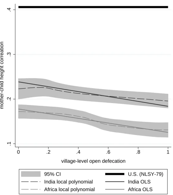
Figure 8 plots mother-child height correlations from the Indian and African DHS samples used in this sample, and for the U.S. from the National Longitudinal Study of Youth 1979. NLSY data used span several calendar years; each child’s height is used in the year he or she is five years old. The correlation computed from the NLSY, 0.41, is comparable to other correlations computed from developed country data (Livson et al., 1962). It is also consistent with the formula above, if ω = 0.5 and σ2
e is small.
Two conclusions emerge from the figure. First, the correlation computed for Indian children – although greater than that in the African data – is much below the correlation for U.S. children, suggesting that any ρ, a direct causal effect of mother’s height on children’s height, may not be large. Second, the correlation between mothers’ and children’s height is lower, within both India and Africa, in villages with more open defecation, which is consistent with an important role for σ2e and with Martorell et al.’s (1977) conjecture that environmental variation will be more important relative to genetics in poorer places.
25Perhaps environmental conditions were so consistently bad in past generations that intrauterine
restric-tion on fetal growth due to large intergenerarestric-tional differences in environmental condirestric-tions were not a binding constraint.
4.4
Decomposing the gap
Decomposition methods estimate the fraction of a difference between two groups that is statistically explained by differences in other variables (Fortin et al., 2011). Decomposition techniques are commonly applied to wage inequality in labor economics and to demographic rates. Like any econometric analysis of observational data, whether decomposition results have a causal interpretation depends on the context and the sources of variation in indepen-dent variables. This section estimates the fraction of the India-Africa height gap statistically “explained” by differences in village-level sanitation, a main result of the paper.
4.4.1 Methods of decomposition
Three methods of decomposition are used. The first is a straightforward application of regression, as in table 5. I regress
heightivs =αIndias+βopendefecationvsv +Xivsθ+εis, (5)
whereheightivsis the height-for-agez score of childiin village v in samples, either India or
Africa. The coefficient of interest is α, on an indicator variable that the child lives in India. The econometric question is by how much adding a control for village level open defecation shifts ˆα in the positive direction. This is essentially identical to the pooled Blinder-Oaxaca decomposition with an indicator for group membership recommended by Jann (2008). The statistical significance of the change in ˆα is evaluated with a Hausmanχ2 test. Various sets of control variables Xivs are added in turn, which will, in general, change both ˆα and ˆβ.
The second method is a weighted two-way Blinder (1973)-Oaxaca (1973) decomposition, using a Stata implementation by Jann (2008). In particular, having seen in section 4.2 that open defecation has different correlations within and across the Indian and African samples,
I implement Reimers’s (1983) recommendation to first estimate
heightivs =βsopendefecationvs +Xivsθs+εis, (6)
separately for each samples, and then compute the difference in height “explained” by open defecation as
0.5 ˆβIndia+ 0.5 ˆβAfrica
opendefecationv,Africa−opendefecationv,India, (7)
creating a counterfactual “effect” of sanitation by weighting equally the within-sample slopes. The third method is a non-linear decomposition, which computes a new mean for the Indian sample after reweighting to match the African sample’s distribution of a set of ob-servable independent variables.26 In particular, the approach is to construct a counterfactual
mean height of Indian children. First, partition both samples into groups g ∈G(X), which share values or ranges of values of a set of covariates X (which could include measures of open defecation). Next, for each group, compute f(g|s), the empirical density of sample
s∈ {India,Africa} in group g, using sampling weights. Finally, compute the counterfactual
mean
˜
hIndia=
X
g∈G(X)
X
i∈g
f(g|Africa )
f(g|India )wihi, (8)
wherewi is the sampling weight of observationiandhi is the height-for-agez-score of childi
in the Indian sample. The unexplained gap is then ˜hIndia−¯hAfrica.The basic set of reweighting
variables used is village and household open defecation, split into 20 groups corresponding to 10 levels of village open defecation for households that do and do not openly defecate.
26Geruso (2012) recently applied this approach to compute the fraction of the U.S. black-white life
4.4.2 Decomposition results
Table 8 presents the decomposition results. Panel A reports the change in the OLS coefficient on a dummy variable for India when a linear control for village-level open defecation is included, as in table 5. Panel B reports the change in the unexplained difference when open defecation is added to a weighted Blinder-Oaxaca decomposition. Panel C presents counterfactual differences from non-parametrically weighting the Indian sample to match the distribution of village and household open defecation in the African sample.
Columns 1 and 2 present the basic result: the simple sample mean with no controls, with and without adjustment for sanitation. Village-level open defecation linearly explains 99 percent of the India-Africa gap.27 In the Blinder-Oaxaca and non-parametric decomposi-tions, sanitation explains more than 100 percent of the gap; this “overshooting” is plausible because, in addition to having worse sanitation, Indian households are richer, on average, than African households.
The next four pairs of columns similarly find that open defecation explains much of the India-Africa gap after controls are added. Specifically, columns 3 and 4 control for demo-graphic variables before decomposing the remaining gap: sex-specific birth order indicators and an indicator for single or multiple birth.28 Columns 5 and 6 first control for a vector of socioeconomic controls, the same controls used earlier in equation 3. Columns 7 and 8 con-trol for a village-level estimate of infant mortality, computed from mothers’ reported birth
27Household-level open defecation, used instead of village-level, explains 68 percent of the gap, a reminder
of the importance of disease externalities.
28Jayachandran and Pande (2012) note that birth order is a predictor of child height in India (see footnote
10). For example, in the sample of rural children under 5 used here, I find that first children are 0.063 (p= 0.044) standard deviations taller than second children. However, this gap falls to 0.034 (p= 0.275) if controls for village and household open defecation are included (jointly significant withF2≈95), suggesting
that children born into larger households may be more likely to be exposed to environmental fecal pathogens, although various forms of intra-household discrimination surely exist, as well (cf.Jeffery et al., 1989).
Jayachandran and Pande (2012) also find, in their pooled DHS sample, that Indian first-borns aretaller than African first-borns. In the individual-level sample studied here, Indian first-borns are 0.019 standard deviations shorter (a much smaller gap than in the full sample, but still negative); controlling for open defecation, they are 0.133 standard deviations taller, a 0.15 increase similar to those when sanitation is controlled for in table 8. If, for example, IMR is controlled for, Indian first-borns are 0.132 standard deviations shorter than African first-borns, which increases by 0.16 to Indians being 0.025 taller.
history. Finally, columns 9 and 10 control for mothers’ height. Because Indian mothers, like Indian children, are short, Indian children are taller than African children, conditional on their mothers’ height. However, section 4.3 has discussed evidence that this correlation is unlikely to be quantitatively importantly causal, and the counterfactual increase in Indian height from matching African sanitation continues to exceed the original, simple gap to be explained, even after adjustment for mothers’ height.
The level of the India-Africa height gap depends on the particular set of controls added before sanitation is accounted for. However, the counterfactual change in height upon ac-counting for open defecation is strikingly similar across specifications. In particular, the flexible non-parametric decomposition in Panel C might best accommodate any shape of the height-sanitation association. In all cases, non-parametrically matching the African distri-bution of open defecation increases the counterfactual Indian mean height by more than the 0.142 standard deviation simple difference in means.
5
Discussion: How much does sanitation explain?
Several dimensions of variation in open defecation quantitatively similarly predict variation in child height: heterogeneity in aggregated country means, changes within Indian districts, and variation across village-level averages. Moreover, Spears (2012a) and Hammer and Spears (2012) document causally well-identified estimates of effects of sanitation on height. Finally, in the sense of econometric decomposition, exceptionally widespread open defecation can explain much of exceptional Indian stunting. So, how much taller would Indian children be if they enjoyed better sanitation and less exposure to fecal pathogens?
5.1
A linear thought experiment
To answer the question above would require knowing the true average causal effect of open defecation on Indian children. However, one can envision possible answers by comparing a
range of estimates of the association between height and open defecation, each reflecting its own particular context and combination of internal and external validity.
Children in rural India are, on average, 0.142 standard deviations shorter than children in the rural African sample in section 4; open defecation is 31.6 percentage points more common in India. Therefore, imagining a linear causal effect of sanitationβ, the fraction of the rural India-Africa height gap that open defecation rates would explain would be whatever fractionβ is of a 0.45 (= 0.142÷0.316) standard deviation increase in height resulting from moving from 100 percent to 0 percent open defecation. Children in India, where 55 percent of households openly defecated in the DHS, are about 2 standard deviations shorter than the reference mean. Whatever fraction β is of 3.6 would be the fraction of the India-U.S. gap explained.
Table 9 collects estimates of the linear association between height and open defecation from this paper and others. As in section 4.4.2, “explaining” over 100 percent of the gap is plausible because wealth differences predict that Indian children should be taller than African children. Unsurprisingly, the instrumental variable treatment-on-the-treated estimate in Hammer and Spears’s (2012) small experimental sample has a large confidence interval. Both this estimate and Spears’s (2012a) may overstate the direct effect of latrines per se
because the programs studied also promoted use of existing latrines.
Like many regression estimates of the effects of inputs on human capital, some of these may be biased upwards. Collectively, however, they suggest that the best linear approxima-tion to the true average causal effect of village-level sanitaapproxima-tion coverage on Indian children’s height is likely to be a large fraction of 0.45 (ignoring the additional explanatory power of population density). If so, then sanitation could explain much or all of the difference in heights between Indian and African children.
5.2
Conclusion: Stunting, “malnutrition,” and externalities
Section 4.1 presented evidence that one household’s open defecation imposes negative exter-nalities on its neighbors. Village-level exterexter-nalities are important for at least two reasons. First, negative externalities are a classic rationale in public economics for government in-tervention: if households do not consider the effect of their own open defecation on other people, they will be too reluctant to switch to using a latrine. Second, statistical approaches that only study private resources will be unable to fully explain heterogeneity in height. For example, Tarozzi (2008) finds that even Indian children in the richest households in the NFHS (that is, with the most assets) are still shorter than international reference norms. Panagariya (2012) interprets this result to suggest that international norms are incorrect for Indian children, because even children with “elite or privileged” household health inputs are stunted.29 Yet, this interpretation ignores externalities: many of the asset-rich households in the NFHS are exposed to a disease environment created by the open defecation of other households. Bhandari et al. (2002) study the height of Indian children living in Green Park, a single affluent neighborhood in South Delhi; these children grow to international reference heights.
Although a child’s low height-for-age is often called “malnutrition,” Waterlow (2011) has advocated instead using “the term ‘stunted,’ which is purely descriptive and does not prejudge the question of whether or not the growth deficit is really the result of malnutri-tion,” often narrowly interpreted as food, especially in policy debates. Early-life disease – and especially chronic disease due to fecal pathogens in the environment – appears to be another important determinant of height. If so, determining whether open defecation is an importantly binding constraint on Indian children’s height may be a step towards a policy response able to resolve this Asian enigma.
29Tarozzi does recognize that his approach does not capture important effects of “the epidemiological