Is Housing Overvalued?

Research

Discussion

Paper

Is Housing Overvalued?

Ryan Fox and Peter Tulip

research so as to encourage discussion and comment. Views expressed in this paper are those of the authors and not necessarily those of the Reserve Bank. Use of any results from this paper should clearly attribute the work to the authors and not to the Reserve Bank of Australia.

The contents of this publication shall not be reproduced, sold or distributed without the prior consent of the Reserve Bank of Australia.

ISSN 1320-7229 (Print) ISSN 1448-5109 (Online)

Ryan Fox* and Peter Tulip**

Research Discussion Paper 2014-06

July 2014

* Financial Stability Department ** Economic Research Department

Reserve Bank of Australia

Thanks to Tom Cusbert, Luci Ellis, Richard Finlay, Alex Heath, Jonathan Kearns, Christopher Kent, David Lancaster, Tony Richards, Nigel Stapledon, Iqbal Syed, Chris Stewart and Marc-Oliver Thurner for helpful comments and discussions. We would like to acknowledge earlier RBA research by Robert Johnson. Views in this paper are those of the authors and not necessarily those of the Reserve Bank of Australia.

Authors: foxr and tulipp at domain rba.gov.au Media Office: [email protected]

i

This paper examines whether it costs more to own a home or to rent. We argue this is a useful criterion for assessing housing overvaluation. We use a new Australian dataset, which includes prices and rents for matched properties, letting us value housing in levels. We find that if real house prices grow at their historical average pace, then owning a home is about as expensive as renting. If prices grow more slowly, as some forecasters predict, the framework used in this paper suggests that the average home buyer would be financially better off renting. We decompose house prices into contributions from rents, interest rates and expected capital gains, which may help policymakers in the detection of housing bubbles. Recent data do not show signs of a bubble.

JEL Classification Numbers: R00, R21

ii

1.   Introduction 1  

2.   Previous Research 4  

3.   The User Cost of Housing 6  

4.   Data Summary 8  

5.   Estimates 10  

5.1   Current Estimates 10  

5.2   Historic Estimates 11  

5.3   Break-even Appreciation Rates 15  

5.4   Discounted Cash Flows 18  

6.   Decomposing Changes in House Prices 20  

7.   Sensitivity 22  

7.1   Capital Appreciation 22  

7.2   Length of Tenure 26  

8.   Conclusion 27  

Appendix A: Data Details 28  

Is Housing Overvalued?

Ryan Fox and Peter Tulip

1.

Introduction

This paper examines whether it is more expensive to own a house or to rent. We assess houses as ‘overvalued’ if home buyers pay too much, in the sense that they would be better off renting than buying. This involves comparing the financial cost of renting a home with the cost of owning a similar dwelling, where the latter depends on the purchase price, interest rates, repairs, council rates and so on. We briefly also examine non-financial costs but find these are small, on average.

We decompose housing values into contributions from rents, interest rates, expected appreciation and other factors, which we hope will be directly useful to potential buyers. The decomposition may also be useful to market participants, policymakers and others who need to understand the reasons for house price movements. For example, we find that the boom in house prices in 2002–2003 can largely be attributed to expectations of further capital appreciation.1 _{That has} implications for lending and prudential standards. Interest rates and rents have been more important determinants of house prices at other times, with a different set of policy implications. Our estimates can be readily updated, which may assist in the early detection of bubbles.2

Given that the supply of housing is fixed in the short run, prices are determined by how much buyers are willing to pay. Hence a comparison of the costs of home ownership with the costs of the nearest alternative seems central to a measure of overvaluation. In contrast, other popular measures of overvaluation, such as the price-to-income ratio, are not obviously a part of any individual’s decision-making process. We compare various measures of overvaluation in the next section.

1 We follow common usage in using the term ‘house prices’ to refer to both detached houses and units except when the distinction is material.

2 Stiglitz (1990, p 13) defines a bubble: ‘if the reason that the price is high today is only because investors believe that the selling price will be high tomorrow—when “fundamental” factors do not seem to justify such a price—then a bubble exists’.

As we discuss in Section 2, our paper contributes to a large literature that compares house prices to rents and the user cost of housing (a term we define precisely in Section 3). Our paper is unusual, though not unique, in two important respects. First, we focus on conditions in Australia. Second, we use a new dataset that matches prices with rents for a large representative sample of properties. In contrast, most previous comparisons of the cost of owning and renting have used different and inconsistent data sources for house prices and rents. Because houses that are bought differ from those that are rented, in both observable and unobservable ways, it has been difficult to discern whether differences in cost reflect differences in quality. Accordingly, researchers could only compare

changes in prices with changes in rents. Even then, they have needed to assume

that quality changes are controlled for similarly in the two series. This assumption becomes increasingly doubtful over longer periods. In contrast, our matched data enables comparisons of the level of prices with the level of rents. Hence, we can estimate the level of overvaluation. It also facilitates an analysis of other interesting properties of dwelling prices, such as their implications for expected capital appreciation.

To summarise our results, we find that assessments of house prices are sensitive to assumptions about expected capital gains. If real house prices were to continue to grow at the average rate of the past six decades, then buying a house now would be about as costly as renting. To put this another way, the expectations of future capital gains implied by current house prices are in line with historical norms. That allays some concerns about a housing ‘bubble’. If house price growth were to be slower than the historical average, as some forecasters predict, then the average home buyer would be financially better off renting.3

These findings relate to average housing conditions, around which individual circumstances will differ. For example, a household expecting historically average capital appreciation will be better off owning than renting if it values home ownership for non-financial reasons, if it expects to remain in the house for longer than average, or if it has substantial financial savings that it cannot profitably invest elsewhere. Given that individual circumstances vary, no-one should base personal investment decisions solely on our estimates. However, we do hope that

3 Full disclosure: during the preparation of this paper one of the authors, Peter Tulip, bought a house. The other author, Ryan Fox, continues to rent.

our approach provides a guide to how these decisions could be made. We also hope that our detailed estimates, which are based on average conditions, are useful when information on individual conditions is unavailable.

Several limitations of the paper (shared by other research on the user cost) are worth noting. First, our analysis is partial equilibrium. We focus on the home-buying decision; this involves comparing prices to rents and expected appreciation, which we take as given. Comparisons of prices to other benchmarks would be relevant to other decisions. For example, a comparison of prices to construction costs would be relevant to builders. Comparing current prices to future prices would be relevant to deciding when to buy or sell. A general equilibrium analysis would explore how all these decisions might be made consistent. But these comparisons are beyond the scope of this paper. Put slightly differently, we examine whether house prices are in line with rents. A broader study could examine whether housing prices and rents are jointly over or undervalued relative to other consumer prices.

Second, we only examine purchases by owner-occupiers, who account for two-thirds of all dwellings. Investors make similar decisions, but these are complicated by taxes.

Third, we focus on whether households are financially better off buying or renting their house and by how much. The decision to buy rather than rent also reflects subjective factors that are difficult to measure such as security of tenure, freedom to renovate, access to finance, pride of ownership, the risk of capital losses and the flexibility of moving. However, although these considerations are important at an individual level, at an aggregate level they seem to cancel out. As we discuss in Section 5.2, non-financial considerations do not seem to have a substantial effect on the average price level. Even if they did, it seems neither useful nor feasible to tell households what their subjective preferences are. In our view, it is informative to calculate average financial costs – about which potential buyers are presumably interested – and let individuals decide for themselves whether these are worth incurring.

2.

Previous Research

Perhaps the most common method of assessing whether house prices are overvalued is to compare the price-to-income ratio with its longer-term average. On this basis, The Economist (2013) and the OECD (2013) report that Australian house prices are 24 per cent and 21 per cent ‘overvalued’, respectively. A limitation of the price-to-income ratio is that its purpose is unclear. Being told that a house is expensive relative to incomes does not tell you whether the purchase is sensible. For that decision you need to know the cost of the alternative.

The price-to-income ratio could be used as a guide to future price movements if the series was mean-reverting. But in Australian data, it is not. Stapledon’s (2012, Figure 3) measure of house prices has risen faster than incomes in each of the past six decades. A trending ratio means recent levels will be persistently higher than the average and that the reported overvaluation will grow over time. It is possible to find definitions of prices and incomes such that their ratio is flat over some periods, but these measures trend strongly at other times.

A trending price-to-income ratio is not surprising. An upward-trending ratio is to be expected when land is in limited supply. Then, as income (and hence the demand for housing) grows, both prices and rents increase. Because demand for housing is price-inelastic, prices need to rise faster than incomes to keep demand in line with supply. A persistent movement in the opposite direction would be expected when extra land becomes freely available, as in the first half of the twentieth century. Fox and Finlay (2012) discuss price-to-income ratios in greater detail.

Another popular approach is to compare price-to-rent ratios to their long-term averages. On this basis, The Economist (2013) and the OECD (2013) conclude that Australian house prices are 46 per cent and 37 per cent ‘overvalued’, respectively. These comparisons are incomplete. Potential home buyers look not just at the price of a house, but also at interest rates, running costs and other elements of the user cost of housing. The price-to-rent ratio is not stationary, but moves with these variables. Indeed, the price-to-rent ratio in Australia has increased over the past few decades, reflecting a decline in the user cost. Unless the user cost is expected to revert to its average, neither will the price-to-rent ratio. Gallin (2008) finds that

the price-to-rent ratio, by itself, is useful for forecasting future house prices in the United States. However, we have not found that for Australia.

For these and other reasons, a large body of research compares the user cost of housing with rents. Often, but not always, this work is motivated by the desire to detect a ‘bubble’ in house prices. To give some illustrative examples, Baker (2002), McCarthy and Peach (2004), Himmelberg, Mayer and Sinai (2005) and Gallin (2005, from whom we copy our title) value houses using the user cost in the United States. Hatzvi and Otto (2008), Weeken (2004), Kivistö (2012) and Browne, Conefrey and Kennedy (2013) conduct similar exercises for Australia, the UK, Finland and Ireland respectively. The OECD (2005) provides international comparisons, including simple estimates for Australia. These papers provide citations to many others. A limitation of these papers is that prices and rents come from different samples with different characteristics. Owner-occupied houses tend to be larger and more expensive than rental dwellings. So a comparison of average prices with average rents reflects quality differences. This problem can be addressed by focusing on changes. Or, more commonly, the focus is on deviations from the average, on the questionable assumption that houses are fairly valued on average.

Our work differs in that we measure rents and prices for the same properties. This enables us to hold housing quality constant and hence assess the level of overvaluation. Several studies have also attempted to do this in the United States, including Smith and Smith (2006), Davis, Lehnert and Martin (2008), Campbell

et al (2009) and Garner and Verbrugge (2009). We compare our results to this

work in Section 5.2.

The paper that most resembles ours is Hill and Syed (2012), who examine Sydney house prices for 2001–2009, within a similar framework. Their paper focuses on technical issues relating to the use of hedonic regressions – specifically, imputation of price-to-rent ratios from incomplete data – and implications for the measurement of GDP, issues we do not address. We focus more on data issues, which leads to significant differences from some of their component estimates. For example, Hill and Syed assume no transaction costs or running costs, though we find these to be important. Offsetting these differences, Hill and Syed include land tax (not actually paid by owner-occupiers) and have high assumptions for

depreciation and a risk premium. Some of their key results are similar to ours, as noted in Section 5.2. We hope that close attention to the relevant data increases the confidence that can be placed in these results. It also facilitates variations and extensions.

Other studies of the user cost of housing in Australia include Bourassa and Yin (2006), Stapledon (2007) and Brown et al (2011). Although these papers address somewhat different questions, we rely heavily on their discussion of the data, in particular the historical estimates compiled by Stapledon.

3.

The User Cost of Housing

A comprehensive comparison of the relative costs of owning and renting adds up the discounted costs of each alternative over the period for which a house is expected to be owned. We present and discuss comparisons along these lines in Section 5.4. However, a useful simplification is to compare cash flows and changes in asset values at a point in time.

The annual cost of owning a home can be written as

(

)

(

)

Cost in dollars =P r c s d+ + + −

_π

where P represents the price of the property; r the real interest rate (a composite of the mortgage rate and the opportunity cost of owner’s equity); c represents other running costs, such as repairs, rates and insurance, as a proportion of the price; s represents buying and selling costs (stamp duty, agent commission, etc.), also as a proportion of the price, averaged over the period of home-ownership; d is the physical depreciation rate; and π is the expected real appreciation rate of the property on a constant-quality basis (that is, excluding the effects of improvements and depreciation). In contrast to other countries, the Australian income tax code does not directly affect the cost of housing for owner-occupiers. The nearest exception is local government rates, which we include in running costs. Our division into five components is for presentational convenience. In Appendix A we show a decomposition with many more elements.

It is convenient to express the annual cost as a percentage of the value of the property, which we will refer to as the user cost:

.

user cost Cost P r c s d= = + + + −

_π

(

)

P r c s d+ + + −

π

where prices, rents and other terms are measured for similar properties. Under assumptions we discuss and relax below, both sides of the equation can be assumed to be approximately constant over the period of ownership.

Equation (3) implicitly defines a ‘fundamental’ value for housing, P*, at which a household is financially as well off buying or renting.

(

)

*

P ≡rent r c s d+ + + −

π

Equation (4) is similar to the widely-used Gordon model of share price valuation, which compares the corporate earnings (or dividend) yield to the risk-free interest rate and other related terms. In analysing share prices it is common to assume that expected prices represent a solution to the same problem, but we follow other papers in the housing literature, which treat expected capital gains as separately determined. Equity pricing equations typically include a risk premium, which we discuss in Section 5.3.

P/P* represents a measure of overvaluation, which, after re-arranging terms, can conveniently be expressed as the ratio of the user cost to the rental yield:

. *

P r c s d user cost Overvaluation

rent

P rental yield P

π

+ + + −

= = = (5)

The equations above involve several simplifications. First, they ignore changes in the user cost over the period of home ownership. That is not a concern if all flows are constant, which is a reasonable assumption for most variables if they are

measured in real terms.4 _{If measured in nominal terms, rents would be expected to} rise in line with inflation, though the nominal interest payments on a loan would not. Strictly speaking, flows cannot be constant if there is real capital appreciation, which involves changing relative prices. It would be more accurate to allow for changing relative prices, to replace _π with _π / (1 + r), discount the selling cost component of transactions costs, and so on. But these complications do not greatly matter, as we show in Section 5.4.

Second, we assume that government programs that influence the cost of home ownership, such as First Home Owners Grants or the exemption of housing from some means tests, are small enough to be ignored.

A more important simplification is that we take rent and expected capital appreciation as exogenous. This approach, standard in the literature cited in Section 2, is partial and may seem inconsistent: the household is assuming that future home buyers solve a different problem to that being considered here. A more complete treatment would explain rents and expected appreciation within a model of the demand and supply of housing, as noted in the introduction. Assuming that expectations are consistent with that model would simplify the analysis, but would also make it difficult to discuss bubbles.

4.

Data Summary

The credibility and usefulness of our estimates hinge on the quality of our data. However, a detailed discussion of measurement issues takes considerable space, which we leave to Appendix A. That discussion includes our treatment of historical estimates. In this section, we provide a brief overview of current estimates.

An important feature of our dataset is that it contains matched prices and rents for the same properties. Rents are obtained by RP Data-Rismark from listings on major real estate websites, which cover almost all properties advertised for rent in major Australian cities. RP Data-Rismark also estimate prices for these same

4 In Australian data, variations in the growth of real rents have been small. This contrasts with the growth in corporate earnings, which is volatile and difficult to predict. So whereas research on equity valuation often solves for the expected growth in earnings, estimates of housing valuation can assume expected rental growth is given.

properties, as explained in Appendix A. As a simplification, if the property has been sold within the previous ten years, the sale price is brought up-to-date by multiplying it by the change in a hedonic price index since the time of the sale. In the absence of a recent sale, the price is imputed by detailed hedonic regressions. For interest rates, we use the average fixed 10-year mortgage rate, less a term premium of 1.3 percentage points. (Like other measurement details, this estimate is discussed in Appendix A.) To express this in real terms, we subtract financial market inflation expectations over the next ten years, derived from swaps markets. We assume that the opportunity cost of owner’s equity is close to the real mortgage rate, so leverage can be ignored.

Our estimates of running costs are based on expenses that landlords claim against rental income on their tax returns. The largest of these are council rates, repairs, and expenditure on furnishings and equipment. We exclude expenses that would be paid by investors but not owner-occupiers, such as property agent fees and land tax. We assume the remaining expenses are representative of what owner-occupiers would also expect to pay, on average.

The most important transaction cost is stamp duty, rates for which we obtain from state revenue offices. We base our estimates of other transaction costs (selling commissions, conveyancing, etc) on discussions with industry contacts. We amortise transaction costs over ten years, the median tenure of home ownership. Our estimates of depreciation come from Stapledon (2007). We measure capital appreciation on a constant-quality net-of-depreciation basis (to be comparable with rental data, in principle), which means the estimates of depreciation have no net effect on the user cost.

In contrast to other studies, we do not explicitly include a ‘risk premium’. It is not clear that the financial risks of home ownership should outweigh renters’ insecurity of tenure and uncertainty regarding future rents, or how this might be quantified. Moreover, aversion to risk is just one of many unobserved subjective factors that may influence the decision to buy a house. We prefer to calculate expected returns and allow households to compare these with their own weighting of subjective factors. We do, however, calculate a rental premium in Section 5.3 which

encompasses attitudes to risk and other non-financial considerations, and find this to be small, on average.

Whereas the above elements of the user cost can be observed or estimated with some confidence, the expected rate of capital appreciation cannot. A variety of assumptions can be made for this variable, as we discuss in more detail below.

5.

Estimates

5.1 Current Estimates

Table 1 shows estimates of parameters and overvaluation for April 2014. In the absence of reliable estimates for _π, the expected rate of real appreciation, the table shows two illustrative values of this parameter. We discuss other plausible assumptions in Section 7.1.

The first column in Table 1 assumes home buyers expect real constant-quality house prices to rise by 2.4 per cent a year, their average rate of increase since 1955. On this assumption, in April 2014, the cost of owning was the same as that of renting, 4.2 per cent of the value of the house. That is, houses are fairly valued. A long-term average provides a clear, simple reference point. However, many (though not all) forecasters believe that house prices are likely to grow at a somewhat slower rate in the future. An investigation of the merits of different forecasts is outside the scope of this paper. However, to illustrate, we use the average of the past ten years, 1.7 per cent, in the second column. For reasons discussed below, the ten-year average is not a good rule for forecasting prices, however, it currently may be closer to a consensus assumption than the post-1955 average, and it has other advantages, some of which are noted in Section 5.3. On this basis, the annual cost of owning a house would have been 4.9 per cent of the value of the property, 19 per cent greater than the 4.2 per cent cost of renting.

The estimates in Table 1 are our central results, which we restate in Section 8 after considering some variations and technical details.

Table 1: Home Price Valuation – April 2014

Per cent of dwelling price

Estimate

Post-1955 expectations

Ten-year average expectations

Real interest rate (r) 3.3 3.3

Running costs (c) 1.5 1.5

Annual average transaction costs (s) 0.7 0.7

Depreciation (d) 1.1 1.1

Expected appreciation (π)

1955–2014 average 2.4

2004–2014 average 1.7

Total user cost (r + c + s + d – π) 4.2 4.9

Average rental yield (rent / P) 4.2 4.2

Overvaluation

as per cent of fundamental value *

* P P P −

⎛ ⎞

⎜ ⎟

⎝ ⎠

0 19

Notes: The bottom row subtracts 1 from Equation (5) to express the degree of overvaluation as per cent of the fundamental value; other variables are defined in the text

Sources: see Appendix A

5.2 Historic Estimates

In deciding whether to buy a house, current estimates of the parameters, as shown in Table 1, are relevant. However, to interpret buyer behaviour and assess the dynamics of the housing market, time series are useful. We expect these historical comparisons to be of direct interest to policymakers but only indirectly to individual home buyers, in so far as it helps them assess the estimates in Table 1. The three panels of Figure 1 extend entries in Table 1 back in time. In general, we consider our recent data to be good, with the exception of estimates of capital appreciation. As we go back in time, data quality deteriorates. Our estimates at the beginning of our sample are of marginal quality; whereas estimates for earlier periods do not seem worth showing.

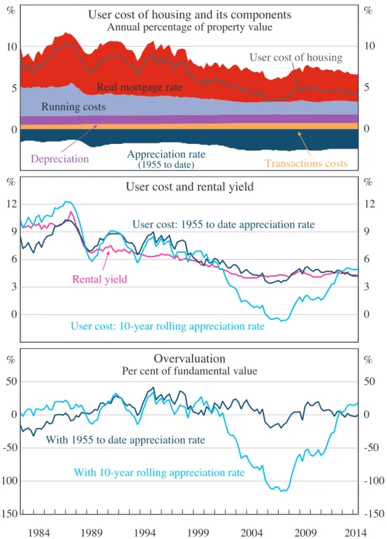
Figure 1: Historical Estimates of the User Cost and its Components

The top panel shows components of the user cost (measured as a percentage of the property value). To reduce clutter, this panel only shows estimates for one proxy for capital appreciation: the average rate of appreciation from 1955 to the date of sale. The middle panel shows (in dark blue) the measure of user costs from the top panel together with the measure that proxies expected appreciation with a 10-year rolling average (in light blue). We also show the average rental yield. The bottom

0 5 10 %

User cost: 1955 to date appreciation rate

Overvaluation Per cent of fundamental value 0 3 6 9 12 0 3 6 9 12 -150 -100 -50 0 50 -150 -100 -50 0 50 2014 User cost of housing and its components

Annual percentage of property value

User cost of housing

Appreciation rate

(1955 to date) Real mortgage rate Running costs

Depreciation _{Transactions costs}

%

% %

% %

User cost and rental yield

Rental yield

User cost: 10-year rolling appreciation rate

With 10-year rolling appreciation rate With 1955 to date appreciation rate

2009 2004 1999 1994 1989 1984 5 0 10

panel shows estimates of overvaluation using the measures of user cost shown in the middle panel. Positive estimates represent overvaluation, that is, the amount that home buyers are paying in excess of what they would pay to rent a similar house.

We make five observations about Figure 1. First, as shown in the bottom panel and discussed further in Section 7.1, estimates of the extent or even direction of overvaluation are sensitive to assumptions about capital appreciation. This point is emphasised in many of the papers mentioned in Section 2.

Second, in contrast to estimates at a point in time, conclusions relating to longer periods are more robust to assumptions about expectations. For both proxies, estimates of overvaluation fluctuate around zero. There has been no clear tendency of Australian houses to be overpriced or underpriced, and the level of overvaluation, when averaged over a long time span, has been small.

An equivalent way of saying this is that the rental yield, on average, is similar to the user cost, as shown in the middle panel. Indeed, if we focus on long-run historical expectations, the relationship between these series is surprisingly close. There is substantial year-to-year volatility, but in the medium term, prices seem well-explained by rents and the user cost. This applies to both levels and changes. More formally, prices, rents and the user cost appear to be cointegrated in logarithms. That implies that measures of overvaluation should be useful for forecasting, though investigating that question is beyond the scope of this paper. This result has implications for the importance of non-financial factors (an awkward term for factors that may lead one to rent or buy even when the expected financial costs might suggest otherwise). Some households prefer to own than rent because they want security of tenure and the freedom to renovate. Others choose to rent due to risk aversion and limited access to credit. The value of these non-financial considerations can be assessed by the amount that households are prepared to pay for them, represented by the wedge between the rental yield and the user cost. The small size of this wedge, when averaged over time, suggests that the average value of these non-financial considerations has been small. Presumably, the factors that have led some households to rent have been offset by

factors that incline other households toward owning. We further discuss (and measure) non-financial considerations in the next section.

Third, as can be seen in the middle panel, the rental yield trends down over our sample. Hence, studies that compare recent levels of this ratio or its inverse to its historic mean, such The Economist (2013) or the OECD (2013), will persistently find large ‘overvaluation’. This downtrend in rental yields has been matched by similar downtrends in the user cost (middle panel), in turn largely reflecting a downtrend in real mortgage rates (top panel). Measures of overvaluation (bottom panel) are trendless.

Fourth, our measures of overvaluation can be compared to others’ estimates. Our measure of overvaluation based on long-run expectations shows similar movements to Hill and Syed’s (2012, Table 9) preferred measure (with 20-year expectations) for Sydney between 2001 and 2009. Like them, we find prices overvalued in the early 2000s, becoming undervalued in the second half of the decade, then switching back to overvalued following the global financial crisis. More important, we share their assessment that the average deviation from financial fundamentals has been small.

These findings for Australia contrast with results for the United States from studies that also use matched prices and rents. Smith and Smith (2006, Figures 8 and 9), and Garner and Verbrugge (2009, Figure 7) find that US houses have tended to be undervalued by large margins. Smith and Smith’s conclusion is disputed by their discussant, Mayer. Although there are many reasons why our results differ from these studies, one important factor is the treatment of expected appreciation, discussed below. As a general observation, these US studies need to be interpreted cautiously given that they find house prices were undervalued near the peak of the US housing boom.

Fifth, a striking feature of the bottom panel is that prices are more than 100 per cent undervalued in 2006 when expectations are proxied by a ten-year average. Over the ten years to 2006, real house price appreciation averaged 6½ per cent a year. This exceeded other components of the user cost, so the total user cost was negative, as shown in the middle panel. Interestingly, Garner and Verbrugge (2009, Figure 7) also estimate negative user costs in the United States at this time,

reflecting high expected capital appreciation. Taken at face value, these estimates imply that, given the large capital appreciation, people could expect to live in their house for free. Whether such an expectation is plausible is controversial: in standard models it would imply demand becomes infinite.

We are sceptical of estimates of overvaluation at a point in time where expectations are proxied by a short rolling average. This approach leads to conclusions that housing is undervalued at the peak of the bubble. Nevertheless, this assumption is standard in the literature. Among Australian studies, Brown

et al (2011) use a 5-year average, Bourassa and Yin (2006) use a 3-year average,

and Hill and Syed (2012) use 10-year and 20-year averages. Similarly, Himmelberg et al (2005) use a 5-year average in the United States, Browne

et al (2013) use a 4-year average in Ireland, and Kivistö (2012) uses a 5-year

average in Finland. Muellbauer (2012) discusses this issue and suggests using a 4-year average.

5.3 Break-even Appreciation Rates

Because of the difficulties in measuring expectations, an attractive benchmark for assessing home values is the break-even rate of appreciation. If we solve Equation (3) for π, we get the rate of appreciation that makes the financial returns from buying equal those from renting. That is:

. B _{r c s d rent P}

π

This break-even rate is shown as the light blue line in Figure 2.

The April 2014 break-even appreciation rate indicates that housing is a profitable investment if real house prices are expected to rise by more than 2.4 per cent per annum. Because it does not require an assumption about expected capital gains, the break-even rate is a clearer and less ambiguous summary measure of our results than the overvaluation ratio. Accordingly, we use it in our sensitivity analysis below. But one should not overstate this benefit, given that it is difficult to assess whether a particular break-even estimate is high or low without some reference to historical appreciation rates. For example, the most recent break-even rate of 2.4 per cent equals the long-run average rate of capital appreciation, (consistent

with the estimate of zero overvaluation reported in Table 1), and is somewhat greater than the ten-year average of 1.7 per cent.

Figure 2: Future Real Capital Appreciation Rates

Although McCarthy and Peach (2004), Hill and Syed (2012, Section 6.2), and others use the break-even rate as a measure of expectations, it could be biased. A difference in the cost of renting and owning – and hence a difference between the break-even rate and expectations – can be sustained indefinitely if there are non-financial benefits or costs of owning relative to renting. However, it is possible to adjust the break-even rate for these non-financial considerations, and hence reduce the bias. On the assumption that household tastes are fairly stable over time, non-financial benefits can be quantified as the average premium that renters are willing to pay, over and above the cost of home ownership. This rental premium is analogous to premiums paid for risk or liquidity studied in the finance literature. As discussed in the previous section, non-financial benefits seem to be small, on balance. For either measure of expectations, the financial costs of owning shown in the middle panel of Figure 1 have, on average, been close to the financial costs of renting. To estimate the premium more precisely, we take historical averages as representative of typical returns. That is a strong assumption, but standard in the financial literature and the research cited in Section 2. We also need to make an

-2 -1 0 1 2 3 4

-2 -1 0 1 2 3 4 % Expected

2014 2009

2004 1999

1994 1989

1984 %

assumption about a proxy for the expected rate of capital appreciation. For this purpose a rolling ten-year average has several advantages over the post-1955 average. First, it is less susceptible to bias arising from structural breaks. Second, a rolling average weights observations over the sample evenly, whereas the long-run mean overweights the relatively subdued appreciation in the early part of the sample. Third, the ten-year average more closely corresponds to the ex post, or realised, cost of ownership.

On that basis, the annual cost of owning, shown as the light blue line in the middle panel of Figure 1 has averaged 5.8 per cent since 1982. This is about 0.4 percentage points less than the cost of renting (the pink line in the same panel), which has averaged 6.2 per cent. That is, on average, renters have been prepared to pay marginally more than owners. This result has surprised some home owners, who consider the non-financial benefits of ownership to be widely valued. However, it is qualitatively consistent with previous research (for example, Hill and Syed (2012), OECD (2005)), where a substantial risk premium is assumed. We take this average as an estimate of the non-financial benefits of renting. However, given the low quality of our early data and the extent of serial correlation, we would not place confidence in the precise point estimate or even its sign. However, the broader point, that the premium is small, is more robust to alternative expectational assumptions and variations in the sample.

Algebraically, the rental premium can be considered as an extra cost of ownership. If we add the premium to the left-hand side of Equation (3) and solve for π, we get the expected rate of capital appreciation that makes households indifferent between owning and renting:

.

e _{r c s d rent P premium}

π

Implicitly, we are assuming that the average non-financial benefits of renting relative to owning are constant over time, with otherwise unexplained price movements being attributed to expected capital gains. _π e is shown as the dark line in Figure 2, calculated assuming a constant rental premium of 0.4 per cent of the value of housing. Under these assumptions, the latest (April 2014) estimate of expected appreciation rounds up to 2.9 per cent. This is higher than the break-even rate, because buyers need compensation for the risks and hassle of ownership. If

potential home buyers expected house prices to rise faster than 2.9 per cent, then buying would be more attractive than renting, and buyers would bid up prices until the adjusted break-even rate matched their expectations.

Muellbauer (2012) argues that central banks should regularly survey home buyers regarding their expectations for capital appreciation. He argues that early detection of an imminent housing ‘bubble’ would facilitate macroeconomic stabilisation and prudential policies. He notes that simple measures – such as the change in house prices – which can be driven by changes in rents, interest rates and so on, are difficult to use for this purpose. Equation (7) provides another way of addressing this concern. Were our measure of expected capital appreciation to increasingly diverge from historic norms, that could be taken as a sign that optimism about capital gains was becoming self-reinforcing. Attractively for this purpose, Equation (7) can be updated in close to real time.

For example, Figure 2 shows that in 2003 home buyers were acting as though they expected real appreciation of almost 4 per cent a year. This was noticeably above the historical average of actual appreciation. At the time, many observers worried about the development of a housing bubble. Interestingly, buyers seem to have been similarly optimistic at other times, without overly worrying the authorities. We return to the 2003 boom in Section 6.

5.4 Discounted Cash Flows

Equation (3) assumes that each component of the user cost can be expressed as a constant rate. That greatly simplifies the computation and presentation of the results. In a more complicated but realistic model, components change over time and interact. These complications can be addressed by calculating expected cash flows over the period of ownership, discounting and then comparing present values.

To do this, we discount future cash flows at the real mortgage rate, on the assumption that households accommodate variations in cash flow by varying the pace at which their loan is paid off. We assume a house is owned for ten years, the median period of home ownership, after which a real capital gain is realised. We

split transaction costs into buying costs, which occur at the beginning of an occupancy and selling costs, which occur at the end.

Perhaps the most important variation from the previous analysis is that we allow for growth in real rents over the period of ownership. The same forces that give rise to long-run real capital appreciation, specifically growing demand interacting with inelastic supply, would also lead to rising real rents. Indeed, Stapledon’s (2007) historical time series for rents (which splice together the deflator for consumption expenditure on rent with the CPI measure) has increased 1.3 percentage points per year faster than the overall CPI, on average, since 1960. For simplicity, we assume a constant rental yield and solve for the common growth rate in both rents and house prices. As above, running costs are assumed to move in line with rents, and hence house prices.

These changes are small and their net effect is even smaller. The expected increase in real rents and the discounting of selling costs are partially offset by the discounting of capital gains. The net result is to make home ownership slightly more attractive, relative to renting. This can be seen in the break-even rates of appreciation shown in Figure 3. The light blue line reproduces the break-even appreciation rate from Figure 2, calculated using the static model described in Section 3, where the latest estimate, for April 2014, is 2.4 per cent. The orange line shows marginally lower estimates using discounted cash flows, for which the latest estimate is 2.3 per cent.

The insensitivity of our results to changing assumptions about growth in rents contrasts with the literature on stock market valuation, which finds substantial sensitivity to assumptions about earnings growth. The main reason is that studies of equity valuation typically assume that higher growth in earnings feeds back into greater appreciation whereas we do not.

Discounted cash flows provide a more comprehensive, and hence more accurate, measure of the relative costs of renting and owning than the static model. However, given that the results are similar, that distinction is unimportant for most purposes. Moreover, discounted cash flows are difficult to transparently decompose into interpretable components and so do not facilitate understanding or

modification. Accordingly, we focus on explaining variations in the static user cost model (with some exceptions, such as Section 7.2).

Figure 3: Break-even Real Appreciation Rates

6.

Decomposing Changes in House Prices

In Tables 1 and A1 we decompose the level of house prices into component parts. To decompose changes, we rearrange Equation (3), using Equation (7), so that house prices are explained by expected capital gains, the rental premium and other components of the user cost. In logs:

(

)

ln_P ln_rent ln _{r c s d} e _premium .

π

= − + + + − + (8)

Totally differentiating:

ln ln e

d P d rent= +

ψ

ψ

ψ

ψ

ψ π

ψ

where 1

(

)

.

e

r c s d premium

P rent

ψ

π

=− -3 -2 -1 0 1 2 3 4 -3 -2 -1 0 1 2 3 4 %

Discounted cash flows

2014 2009 2004 1999 1994 1989 1984 % Static

The last step uses Equation (7). Equation (9) expresses the proportionate change in house prices as the sum of contributions from changes in rents and the user cost. Changes in components of the user cost are weighted by ψ, the partial derivative of lnP with respect to the corresponding component, which equals minus the price-to-rent ratio.

Figure 4 shows the main elements of Equation (9). We take eight-quarter log differences, then multiply by 100/2 to express as approximate annualised percentage changes. We measure ψ as the average of the values at the start and end of the eight-quarter period. We measure the growth of both house prices and rents in real terms. We do not show the zero contributions of depreciation and the rental premium, the tiny decomposition approximation error (mean zero, standard deviation 0.01 percentage points) or the small contribution from transaction costs (mean –0.12, standard deviation 0.15 percentage points). We show contributions from 1995, when data on 10-year fixed mortgages became available.

Figure 4: Contributions to Real House Price Growth

Annualised two-year changes, log points x 100/2

To illustrate, consider the two years to December 2003, when real house prices grew at a rapid annual rate of about 13 per cent. This increase is not attributable to mortgage rates which increased slightly. Rising real rents and a decline in the rate of running costs made moderate contributions (approximately 4 and 3 percentage

-30 -20 -10 0 10 20

-30 -20 -10 0 10 20 Annualised price growth

December 2003

Q Mortgage rate Q Running costs Q Rent Q Appreciation 2014 2010

2006 2002

points, respectively). As was often suggested at the time (see Bloxham, Kent and Robson (2010, Section 4.1)), most of the increase in prices can be attributed to higher expected capital appreciation. If expected real appreciation had remained at its December 2001 level of 3.2 per cent, instead of rising to 3.9 per cent, annual real house price growth would have been about 8 percentage points less.

More recently, real house prices have risen at an annual rate of 4 per cent in the two years to April 2014. This reflects a decline in mortgage rates (contributing 5 percentage points), which was partially offset by a decline in expected appreciation that subtracted 2 percentage points. The RP Data-Rismark measure of advertised rents rose slightly less than inflation over this period.

7.

Sensitivity

Our baseline results apply to national averages. Potential home buyers will wish to vary these estimates depending on their individual circumstances and judgements. In some cases, this is simple: for example, a household expecting lower running costs or borrowing at a lower-than-average mortgage rate would see their user cost decline one-for-one. In the following sections we discuss two variations that are less straightforward: the expected rate of capital gains (Section 7.1) and the period for which a house is expected to be owned (Section 7.2).

7.1 Capital Appreciation

Figure 5, which shows several measures of house prices, highlights some of the uncertainty about capital appreciation and the range of plausible assumptions. Of particular interest are the estimates of constant-quality prices constructed by Nigel Stapledon in orange, with median house prices in dark blue. As discussed in Appendix A, Stapledon’s constant-quality estimates provide a useful focal point – in part because they are more clearly consistent with other elements of the user cost than other house price measures.

Two observations are worth noting. First, real constant-quality house prices have trended up steadily since the 1950s. Figure 5 uses a log scale to show the similarity of growth rates in different periods. Growth in the second half is slightly faster than in the first half, but the difference is small both in economic terms and relative

to the noise in the data. To be more precise, the series resembles a random walk with relatively constant drift. Second, other data series are available over shorter periods, but show similar trends.

Because real house prices in Australia have continued to rise over a long period of time, induction suggests that this trend will continue. The mean of a long sample provides a simple and transparent first approximation to what should be expected in the future.

Figure 5: Real (2014) Dwelling Prices

Log scale

Sources: ABS; RBA; Real Estate Institute of Australia (REIA); Residex; RP Data-Rismark; Stapledon (2007) However, trends need not be stable. Some observers (e.g. the Financial Stability Review (RBA 2013, p 50) and Ellis (2013)) suggest that capital appreciation in the future may be lower than in the past. Accordingly, Figure 6 shows some alternative benchmarks that house prices might be expected to follow. The blue line shows how estimates of overvaluation would vary accordingly.

The 10-year and post-1955 averages shown in Table 1 have been discussed above. The 30-year average, a benchmark referred to by Ellis (2013), is conceptually similar. Real disposable income per household (labelled ‘HHDY’) has grown at an average annual rate of 1.6 per cent since 1960. Were house prices expected to grow

300

150

75 300

150

75

Stapledon (constant quality)

$’000

2014 $’000

2003 1992

1981 1970

— ABS houses — REIA — Residex — RP Data-Rismark

Stapledon

(median)

at this rate, housing currently would be approximately 20 per cent overvalued. A limitation of this measure is that it excludes population growth. Broader measures of income, such as real GDP, which may be better proxies for overall housing demand, have grown at an average rate of 3.5 per cent since 1960, implying undervaluation. A more theoretically attractive assumption is that house prices grow in line with rents; but again, different measures are available. Real rents measured by the CPI have risen 1.3 per cent since 1960. Real gross rents per dwelling, based on the national accounts (labelled ‘NA rents’), have risen an average of 3.3 per cent.5

Figure 6: Expected Real House Price Appreciation and Overvaluation

April 2014

Forecasts of future price growth should encompass the above measures together with other relevant information. One set of forecasts comes from the 2014:Q1 NAB survey of property professionals, whose respondents project that house prices will rise 2.8 per cent over the next year. It is unclear what definition of prices respondents have in mind, but we suspect it is the price for a ‘given house’, which

5 Estimates of rents are from Stapledon (2007), kindly updated by Nigel Stapledon. There are concerns that the CPI measure has too large an adjustment for quality changes. The national accounts measure is not quality adjusted. An estimate of rental growth consistent with our measure of price appreciation would probably lie between these estimates.

Break-even rate = 2.4%

O O O O O O O O -30 -20 -10 0 10 20 30 40

1.0 1.5 2.0 2.5 3.0 3.5 4.0

Overvaluation – % of fundamental value

Expected real appreciation (annualised) – %

GDP 30-year NA rents Post-1955 10-year HHDY CPI rents NAB Survey

includes wear and tear but excludes improvements. To make this comparable with other estimates, we add our assumption of physical depreciation (1.1 per cent, discussed in Section A.3) and subtract expected inflation (2.8 per cent, discussed in Section A.7), to give an expected rate of real appreciation of constant-quality houses of 1.1 per cent. Were this rate of appreciation to continue, it would imply overvaluation of 32 per cent. The NAB survey provides a direct measure of expectations, which is useful for many purposes, such as analysing buyer behaviour. However, for reasons we discuss in Appendix A.2, it does not seem a reliable indicator of future price changes.

Expectations of professional forecasters avoid some of the problems of the NAB survey.6 _{However, averaging these forecasts is difficult, partly because some} deserve more weight than others. That said, our judgement is that the central tendency of published house price forecasts is probably for moderate real appreciation over the next few years, at a somewhat slower rate than the long-term historical average. This would imply that houses are slightly overvalued. However, there are also reputable forecasts that imply undervaluation, fair valuation and substantial overvaluation.

It could be assumed that the predictions of a well-specified econometric model would appropriately summarise the available information and provide a plausible measure of expectations, or at least, what they should be. However, it is not clear that statistical models provide a plausible basis for decision-making. For example, Garner and Verbrugge (2009) estimate a variety of time series models for US house prices. These models often imply very strong expected appreciation, which in turn implies negative user costs. It is doubtful that US households, as a group, did or should have acted on the assumption that the cost of buying a house was negative. It may be that the accuracy of the models was impaired by the short samples for which some explanatory variables were available.

6 A convenient source for private sector forecasts of property prices is www.propertyobserver.com.au. One of the most widely cited forecasts is that of BIS Shrapnel, reported in Schlesinger (2013).

7.2 Length of Tenure

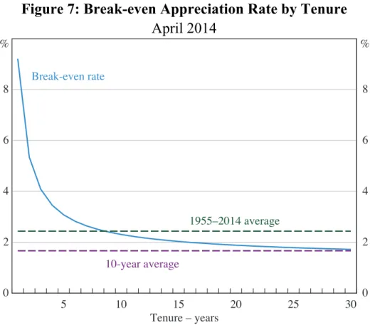
Home ownership is more attractive the longer a house is owned, because transactions costs are amortised over a longer period. However, because housing tenure affects the user cost non-linearly, the size of this effect is not obvious. We show break-even appreciation rates for varying lengths of tenure in Figure 7. Because issues of timing seem central, we use the discounted cash flow model of Section 5.4.

With historical average real house price expectations of 2.4 per cent, represented by the green dashed line in Figure 7, buying is less expensive than renting for anyone expecting to stay in their house for more than eight years. This contrasts with a threshold of ten years using the static model. If real appreciation over the previous 10 years (1.7 per cent) is used as a guide (the purple dashed line), buying is less expensive than renting only with extremely long expected tenure (in excess of 30 years). Consistent with conventional wisdom, households expecting to move again in a few years’ time are better off renting, unless they believe they can sell the property for an unusually large capital gain.

Figure 7: Break-even Appreciation Rate by Tenure

April 2014

1955–2014 average

Tenure – years

5 10 15 20 25 30

0 2 4 6 8

0 2 4 6 8 % %

10-year average

8.

Conclusion

Real house prices have increased at an average annual rate of slightly less than 2½ per cent since 1955. If this rate of appreciation is expected to continue then our estimates suggest that houses are fairly valued (see Table 1 or Figure 3). As we discuss in Section 7.1, forecasting house price growth is subject to considerable uncertainty. That said, many observers have suggested that future house price growth is likely to be somewhat less than this historic average. In that case, at current prices, rents, interest rates and so on, the average household is probably financially better off renting than buying.

Several extensions of our results would be interesting. First, although our paper only reports results for owner-occupiers, we have also examined whether buying a house is worthwhile for investors. This question is complicated by taxes and we have not found a simple way of summarising this. Second, to infer expected capital gains from existing house prices, we assume that the rental premium is constant. Variations in credit restrictions might help to explain variations in the premium over time. Third, whereas we have focused on variations in the user cost over time, cross-section variation could explain who owns and who rents. Fourth, the implications for lending standards might be worth considering. When financial institutions set loan-to-value limits, should the denominator be the fundamental value or the market value? Fifth, and perhaps of most use to potential owners, would be guidance regarding likely capital appreciation. Related to that, our measures of overvaluation may help to predict future house price growth, but that remains to be tested.

Appendix A: Data Details

This appendix discusses our data in detail so as to permit readers to understand, extend and vary our estimates. We also explain why our data choices differ from those others have made. As a roadmap, Table A1 shows a breakdown of components of the user cost in April 2014, assuming expected capital appreciation equals the historical mean. Essentially, this is column 1 of Table 1 in more detail.

A.1 Rental Yields

Since 2010, the RBA has commissioned RP Data-Rismark, a private property data provider, to compile estimates of the average ratio of rents to prices of matched properties.7 _{These estimates have been regularly published by the RBA in its}

Statement on Monetary Policy and other Bank publications. The numerical data are

confidential and available for purchase from RP Data.

For each of the eight capital cities and a national composite we have separate estimates for houses and units. The numerator in each of these estimates equals the sum of annual advertised rent on all properties listed for rent on major real estate websites. These websites cover almost all properties available for rent. The denominator is the sum of imputed prices on those same properties. Imputed prices are a weighted average of two components. The first is the most recent sale price of the property, multiplied by the change in a hedonic price index over the period since that sale. This component receives a weight that declines as the period since the sale increases, reaching zero at ten years. The second component is the prediction of hedonic regressions – that is, the average price at that time for a unit or house in that postcode with the same floor size, bedrooms, bathrooms and other observable characteristics. Sales on nearby properties are given a higher weight in these calculations. The RP databases (like the APM data used by Hill and Syed (2012)) are unusual in that they match administrative data on sale prices with detailed property characteristics from internet advertisements for a near-universal sample.

7 We would like to express our gratitude to Tony Richards and Matthew Hardman, who were instrumental in the creation of this series.

Table A1: Home Price Valuation by Component – April 2014

Per cent of dwelling price

Total

(Table 1 entry)

Average 10-year fixed mortgage rate 7.5

less term premium 1.3

equals average expected mortgage rate 6.2

less expected inflation 2.8

equals Real interest rate (r) 3.3

Council rates 0.3

plus repairs 0.3

plus depreciation on plant 0.3

plus body corporate fees 0.2

plus water 0.1

plus insurance 0.1

plus other running costs 0.2

equals Running costs (c) 1.5

Stamp duty 4.0

plus conveyancing and other buying costs 0.3

equals total buying costs 4.3

Real estate agent commission 2.5

plus advertising, legal and other selling costs 0.5

equals total selling costs 3.0

Total transaction costs 7.3

Average (over ten years) transaction costs (s) 0.7

Depreciation of structure (d) 1.1

Change in real median house price (1955–2014) 3.1

less alterations and additions (1961–2005) 1.1

less high quality/size of new houses 0.9

plus depreciation 1.1

plus change in location 0.4

equals Change in constant-quality prices (π) 2.4

Total user cost (r + c + s + d – π) 4.2

Average rental yield (rent / P) 4.2

Overvaluation as per cent of fundamental value 0

Note: Components may not add exactly to totals due to rounding

P P P < £ ¤

² ¥

¦ ´

* *

Each quarter, about 100 000 advertised rents and the same number of imputed prices enter the rental yield calculation, with houses typically slightly outnumbering units. Details on the hedonic indices and regressions are in Hardman (2011a, 2011b, 2013).

Imputed prices differ slightly from sale prices due to random variation. The regression standard error is about 8 per cent, which might be considered to be reasonably accurate. However, for our purposes what matters is the within-sample mean. By construction, the average imputed price equals the average sale price. Characteristic-specific dummies mean this holds at a highly disaggregated (such as postcode) level. It is possible that rental properties systematically differ in price from owner-occupied properties (and hence from average sale prices) in ways that are not captured by the hedonic regressions. Discussions with real estate agents suggest this is unimportant; consistent with this, previous occupancy status is rarely mentioned in advertisements. In any case, it would be captured in the valuation for those properties where a recent sale is recorded.

Figure A1 shows some estimates of rental yields. Our preferred series is labelled as ‘RP Data-Rismark (rental properties)’. The series labelled ‘RP Data-Rismark (all properties)’ represents slightly different estimates that RP Data publish on their website, which impute rental yields to the total dwelling stock (rather than just properties advertised for rent). The RBA has chosen to emphasise the estimates for rental properties as being more accurate and conceptually simpler. For other purposes, the estimates for all properties might be more representative, though the difference is small.

Because the RP Data–Rismark estimates compare prices and rents for properties of the same quality, they are a dramatic advance on the estimates used by most previous researchers discussed in Section 2, permitting a much broader set of questions to be meaningfully examined. They are quite similar to the estimates of Hill and Syed (2012), which we also show in Figure A1, and, in method of construction, to the estimates of Davis et al (2008) for the United States. Our estimates differ from those of Hill and Syed in several respects, though whether these differences matter may depend on the purpose. Hill and Syed’s estimates are publicly documented in considerably greater detail, including their sensitivity to alternative assumptions. Whereas Hill and Syed’s estimates are for Sydney houses,

the RP Data-Rismark estimates we use are for all capital city dwellings. The RP Data-Rismark estimates benchmark imputed prices to past sale prices for the property; and, importantly for the purposes of the RBA, they are timely, with a one month publication lag.

Figure A1: Rental Yields

Houses and units

Sources: ABS; Hill and Syed (2012); RBA; REIA; RP Data-Rismark; authors’ calculations

The RP Data–Rismark estimates have some limitations. Advertised rents will differ from actual rents; for example, if subsequent adjustments do not equal changes in market rates. Furthermore, using advertised properties means that we weight rental yields by turnover and time on market. This may be unrepresentative of the rental stock in general if properties with unusually high rents are listed for longer or have higher turnover. Hill and Syed (2012, footnote 8) and conversations with real estate agents suggest that these biases are not important.

A more important, practical limitation of the RP Data-Rismark rental yield estimates is that they are only available in consistent form back to 2005. Before then, we splice on estimates from the Real Estate Institute of Australia (REIA) of median rents and median dwelling prices. As noted above, the median dwelling is a more expensive property than the median rental. So the rental yield constructed from REIA estimates is lower than the rental yield from matched properties.

Spliced series used in paper

(see text)

2014 2

4 6 8 10

2 4 6 8 10

REIA

% %

2008 2002

1996 1990

1984

RP Data-Rismark (rental properties)

RP Data-Rismark

(all properties)

Compositional changes will affect the REIA estimates over time, though it is not clear whether these biases are important, or even whether they are positive or negative. For example, the trend increase in the share of unit rentals will impart a downward bias, whereas the increased density of rentals in city centres will impart an upward bias. In the hope that such biases are approximately offsetting, we splice the RP Data-Rismark estimates with level-adjusted REIA estimates to extend the time series back from June 2005 to September 1982.

For Section 6 we require separate estimates of prices and rents. We measure prices using RP Data-Rismark’s hedonic all capital cities dwelling series, and multiply this by the rental yield estimates above to obtain rents.

A.2 Expected Appreciation

The appropriate assumption for expected capital gains will depend on the purpose of the analysis. To examine whether home buyers behave rationally or predictably, a measure of actual expectations is relevant. There are several surveys of house price expectations in Australia, of which the NAB survey of property professionals, discussed in Section 7.1, is probably the most direct. Surveys by Westpac-Melbourne Institute and Mortgage Choice show similar movements, but are harder to summarise as a point estimate. The NAB survey estimates have limitations. Respondents are asked about expectations over the next two years, but it is unclear whether they report a sum or an average. Accordingly we report the one-year-ahead estimate, even though most capital gains will be realised at much longer horizons. We do not know how representative the respondents’ answers are: home buyers may have different expectations to property professionals. Incentives to develop and report accurate expectations are weak. We do not know how these reported expectations have changed over time. We do not know how respondents define ‘house prices’; for example, whether they include improvements or depreciation. Studies in the United States (see Case, Shiller and Thompson (2012) and accompanying comments) suggest that many home buyers have difficulty answering survey questions in a sensible or consistent manner.

To measure overvaluation, or to decide on whether to buy a house, the appreciation rate that should be expected is relevant. If one assumes expectations are rational, or has faith in the wisdom of crowds, this would coincide with actual expectations,