COMPUTER SCIENCE AND TECHNOLOGY 25(4): 615–626 July 2010/DOI 10.1007/s11390-010-1051-1
Dirichlet Process Gaussian Mixture Models: Choice of the Base
Distribution
Dilan G¨or¨ur1 and Carl Edward Rasmussen2,3
1Gatsby Computational Neuroscience Unit, University College London, London WC1N 3AR, U.K. 2Department of Engineering, University of Cambridge, Cambridge CB2 1PZ, U.K.
3Max Planck Institute for Biological Cybernetics, D-72076 T¨ubingen, Germany
E-mail: [email protected]; [email protected] Received May 2, 2009; revised February 10, 2010.
Abstract In the Bayesian mixture modeling framework it is possible to infer the necessary number of components to model the data and therefore it is unnecessary to explicitly restrict the number of components. Nonparametric mixture models sidestep the problem of finding the “correct” number of mixture components by assuming infinitely many components. In this paper Dirichlet process mixture (DPM) models are cast as infinite mixture models and inference using Markov chain Monte Carlo is described. The specification of the priors on the model parameters is often guided by mathematical and practical convenience. The primary goal of this paper is to compare the choice of conjugate and non-conjugate base distributions on a particular class of DPM models which is widely used in applications, the Dirichlet process Gaussian mixture model (DPGMM). We compare computational efficiency and modeling performance of DPGMM defined using a conjugate and a conditionally conjugate base distribution. We show that better density models can result from using a wider class of priors with no or only a modest increase in computational effort.
Keywords Bayesian nonparametrics, Dirichlet processes, Gaussian mixtures
1 Introduction
Bayesian inference requires assigning prior distribu-tions to all unknown quantities in a model. The uncer-tainty about theparametric form of the prior distribu-tion can be expressed by using a nonparametric prior. The Dirichlet process (DP) is one of the most promi-nent random probability measures due to its richness, computational ease, and interpretability. It can be used to model the uncertainty about the functional form of the distribution for parameters in a model.
The DP, first defined using Kolmogorov consistency conditions[1], can be defined in several different per-spectives. It can be obtained by normalising a gamma process[1]. Using exchangeability, a generalisation of the P´olya urn scheme leads to the DP[2]. A closely re-lated sequential process is the Chinese restaurant pro-cess (CRP)[3-4], a distribution over partitions, which also results in the DP when each partition is assigned an independent parameter with a common distribution. A constructive definition of the DP was given by [5], which leads to the characterisation of the DP as a stick-breaking prior[6].
The hierarchical models in which the DP is used as a prior over the distribution of the parameters are re-ferred to as the Dirichlet process mixture (DPM) mod-els, also called mixture of Dirichlet process models by some authors due to [7]. Construction of the DP using a stick-breaking process or a gamma process represents the DP as a countably infinite sum of atomic measures. These approaches suggest that a DPM model can be seen as a mixture model with infinitely many compo-nents. The distribution of parameters imposed by a DP can also be obtained as a limiting case of a parametric mixture model[8-11]. This approach shows that a DPM can easily be defined as an extension of a parametric mixture model without the need to do model selection for determining the number of components to be used. Here, we take this approach to extend simple finite mix-ture models to Dirichlet process mixmix-ture models.
The DP is defined by two parameters, a positive scalar α and a probability measure G0, referred to as the concentration parameter and the base measure, re-spectively. The base distribution G0 is the parameter on which the nonparametric distribution is centered, which can be thought of as the prior guess[7]. The
Regular Paper
This work is supported by Gatsby Charitable Foundation and PASCAL2. ©2010 Springer Science + Business Media, LLC & Science Press, China
concentration parameterαexpresses the strength of be-lief in G0. For small values of α, samples from a DP is likely to be composed of a small number of atomic measures with large weights. For large values, most samples are likely to be distinct, thus concentrated on G0.
The form of the base distribution and the value of the concentration parameter are important parts of the model choice that will effect the modeling performance. The concentration parameter can be given a vague prior distribution and its value can be inferred from the data. It is harder to decide on the base distribution since the model performance will heavily depend on its paramet-ric form even if it is defined in a hierarchical manner for robustness. Generally, the choice of the base distri-bution is guided by mathematical and practical conve-nience. In particular, conjugate distributions are pre-ferred for computational ease. It is important to be aware of the implications of the particular choice of the base distribution. An important question is whether the modeling performance is weakened by using a con-jugate base distribution instead of a less restricted dis-tribution. A related interesting question is whether the inference is actually computationally cheaper for the conjugate DPM models.
The Dirichlet process Gaussian mixture model (DPGMM) with both conjugate and non-conjugate base distributions has been used extensively in appli-cations of the DPM models for density estimation and clustering[11-15]. However, the performance of the mod-els using these different prior specifications have not been compared. For Gaussian mixture models the con-jugate (Normal-Inverse-Wishart) priors have some un-appealing properties with prior dependencies between the mean and the covariance parameters, see e.g., [16]. The main focus of this paper is empirical evaluation of the differences between the modeling performance of the DPGMM with conjugate and non-conjugate base distributions.
Markov chain Monte Carlo (MCMC) techniques are the most popular tools used for inference on the DPM models. Inference algorithms for the DPM models with a conjugate base distribution are relatively easier to im-plement than for the non-conjugate case. Nevertheless several MCMC algorithms have been developed also for the general case[17-18]. In our experiments, we also com-pare the computational cost of inference on the conju-gate and the non-conjuconju-gate model specifications.
We define the DPGMM model with a non-conjugate base distribution by removing the undesirable depen-dency of the distribution of the mean and the covari-ance parameters. This results in what we refer to as a conditionally conjugate base distribution since one of the parameters (mean or covariance) can be integrated
out conditioned on the other, but both parameters can-not simultaneously be integrated out. In the following, we give formulations of the DPGMM with both a con-jugate and a conditionally concon-jugate base distribution G0. For both prior specifications, we define hyperpri-ors onG0 for robustness, building upon [11]. We refer to the models with the conjugate and the conditionally conjugate base distributions shortly as the conjugate model and the conditionally conjugate model, respec-tively. After specifying the model structure, we discuss in detail how to do inference on both models. We show that mixing performance of the non-conjugate sampler can be improved substantially by exploiting the con-ditional conjugacy. We present experimental results comparing the two prior specifications. Both predic-tive accuracy and computational demand are compared systematically on several artificial and real multivariate density estimation problems.
2 Dirichlet Process Gaussian Mixture Models
A DPM model can be constructed as a limit of a parametric mixture model[8-11]. We start with setting out the hierarchical Gaussian mixture model formula-tion and then take the limit as the number of mixture components approaches infinity to obtain the Dirichlet process mixture model. Throughout the paper, vector quantities are written in bold. The indexialways runs over observations, i = 1, . . . , n, and index j runs over components, j = 1, . . . , K. Generally, variables that play no role in conditional distributions are dropped from the condition for simplicity.
The Gaussian mixture model with K components may be written as:
p(x|θ1, . . . , θK) = K X j=1
πjN(x|µj, Sj) (1)
where θj = {µj, Sj, πj} is the set of parameters for componentj,πare themixing proportions(which must be positive and sum to one),µj is the mean vector for componentj, andSjis itsprecision (inverse covariance matrix).
Defining a joint prior distribution G0 on the com-ponent parameters and introducing indicator variables ci, i= 1, . . . , n, the model can be written as:
xi|ci,Θ∼ N(µci, Sci)
ci|π∼Discrete(π1, . . . , πK) (µj, Sj)∼G0
π|α∼Dir(α/K, . . . , α/K). (2)
number of observations assigned to each component, called theoccupation number, is multinomial
p(n1, . . . , nK|π) =
n! n1!n2!· · ·nK!
K Y j=1
πnj
j , and the distribution of the indicators is
p(c1, . . . , cn|π) = K Y j=1
πnj
j . (3)
The indicator variables are stochastic variables whose values encode the class (or mixture component) to which observationyi belongs. The actual values of the indicators are arbitrary, as long as they faithfully rep-resent which observations belong to the same class, but they can conveniently be thought of as taking values from 1, . . . , K, whereK is the total number of classes, to which observations are associated.
2.1 Dirichlet Process Mixtures
Placing a symmetric Dirichlet distribution with pa-rameterα/Kand treating all components as equivalent is the key in defining the DPM as a limiting case of the parametric mixture model. Taking the product of the prior over the mixing proportionsp(π), and the indi-cator variables p(c|π) and integrating out the mixing proportions, we can write the prior on c directly in terms of the Dirichlet parameterα:
p(c|α) = Γ(α) Γ(n+α)
K Y j=1
Γ(nj+α/K)
Γ(α/K) . (4)
Fixing all but a single indicatorci in (4) and using the fact that the datapoints are exchangeable a priori, we may obtain the conditional for the individual indica-tors:
p(ci=j|c−i, α) =n−i,j+α/K
n−1 +α , (5) where the subscript −i indicates all indices except for i, and n−i,j is the number of datapoints, excluding
xi, that are associated with class j. Taking the limit K→ ∞, the conditional prior forcireach the following limits:
components for whichn−i,j>0 : p(ci =j|c−i, α) = n−i,j
n−1 +α, (6a)
all other components combined:
p(ci 6=ci0 for alli6=i0|c−i, α) = α
n−1 +α. (6b)
Note that these probabilities are the same as the proba-bilities of seating a new customer in a Chinese restau-rant process[4]. Thus, the infinite limit of the model in (2) is equivalent to a DPM which we define by starting with Gaussian distributed data xi|θ ∼ N(xi|µi, Si), with a random distribution of the model parameters (µi, Si)∼Gdrawn from a DP,G∼DP(α, G0).
We need to specify the base distributionG0to com-plete the model. The base distribution of the DP is the prior guess of the distribution of the parameters in a model. It corresponds to the distribution of the com-ponent parameters in an infinite mixture model. The mixture components of a DPGMM are specified by their mean and precision (or covariance) parameters, there-foreG0 specifies the prior on the joint distribution of
µ and S. For this model, a conjugate base distribu-tion exists however it has the unappealing property of prior dependency between the mean and the covariance as detailed below. We proceed by giving the detailed model formulation for both conjugate and conditionally conjugate cases.
2.2 Conjugate DPGMM
The natural choice of priors for the mean of the Gaussian is a Gaussian, and a Wishart① distribution for the precision (inverse-Wishart for the covariance). To accomplish conjugacy of the joint prior distribution of the mean and the precision to the likelihood, the dis-tribution of the mean has to depend on the precision. The prior distribution of the meanµj is Gaussian con-ditioned onSj:
(µj|Sj,ξ, ρ)∼ N(ξ,(ρSj)−1), (7) and the prior distribution ofSj is Wishart:
(Sj|β, W)∼ W(β,(βW)−1). (8)
The joint distribution of µj and Sj is the Nor-mal/Wishart distribution denoted as:
(µj, Sj)∼ N W(ξ, ρ, β, βW), (9)
withξ, ρ, β andW being hyperparameters common to all mixture components, expressing the belief where the component parameters should be similar, centered around some particular value. The graphical represen-tation of the hierarchical model is depicted in Fig.1.
Note in (7) that the data precision and the prior on the mean are linked, as the precision for the mean is a multiple of the component precision itself. This depen-dency is probably not generally desirable since it means
①There are multiple parameterizations used for the density function of the Wishart distribution. We use W(β,(βW)−1) = (|W|(β/2)D)β/2
ΓD(β/2) |S|
(β−D−1)/2exp³−β
2tr(SW)
´
, whereΓD(z) =πD(D−1)/4QDd=1Γ
³
z+ (d−D)/2
´
Fig.1. Graphical representation of hierarchical GMM model with conjugate priors. Note the dependency of the distribution of the component mean on the component precision. Variables are labelled below by the name of their distribution, and the parameters of these distributions are given above. The circles/ovals are segmented for the parameters whose prior is defined not directly on that parameter but on a related quantity.
that the prior distribution of the mean of a component depends on the covariance of that component but it is an unavoidable consequence of requiring conjugacy.
2.3 Conditionally Conjugate DPGMM
If we remove the undesired dependency of the mean on the precision, we no longer have conjugacy. For a more realistic model, we define the prior onµj to be
p(µj|ξ, R)∼ N(ξ, R−1) (10) whose mean vectorξand precision matrixRare hyper-parameters common to all mixture components. Keep-ing the Wishart prior over the precisions as in (8), we obtain theconditionally conjugate model. That is, the prior of the mean is conjugate to the likelihood condi-tional onS and the prior of the precision is conjugate conditional onµ. See Fig.2 for the graphical represen-tation of the hierarchical model.
A model is required to be flexible to be able to deal
with a large range of datasets. Furthermore, robust-ness is required so that the performance of the model does not change drastically with small changes in its parameter values. Generally it is hard to specify good parameter values that give rise to a successful model fit for a given problem and misspecifying parameter values may lead to poor modeling performance. Using hierar-chical priors guards against this possibility by allowing to express the uncertainty about the initial parame-ter values, leading to flexible and robust models. We put hyperpriors on the hyperparameters in both prior specifications to have a robust model. We use the hi-erarchical model specification of [11] for the condition-ally conjugate model, and a similar specification for the conjugate case. Vague priors are put on the hyperpa-rameters, some of which depend on the observations which technically they ought not to. However, only the empirical meanµy and the covarianceΣy of the data are used in such a way that the full procedure becomes invariant to translations, rotations and rescaling of the
Fig.2. Graphical representation of hierarchical GMM model with conditionally conjugate priors. Note that the mean µk and the precisionSk are independent conditioned on the data.
data. One could equivalently use unit priors and scale the data before the analysis since finding the overall mean and covariance of the data is not the primary concern of the analysis, rather, we wish to find struc-ture within the data.
In detail, for both models the hyperparameters W and β associated with the component precisions Sj are given the following priors, keeping in mind that β should be greater thanD−1:
W ∼ W ³
D, 1 DΣy
´ ,
³ 1
β−D+ 1 ´
∼ G ³
1, 1 D
´ . (11)
For the conjugate model, the priors for the hyper-parametersξandρassociated with the mixture means
µj are Gaussian and gamma②:
ξ∼ N(µy,Σy), ρ∼ G(1/2,1/2). (12) For the non-conjugate case, the component means have a mean vectorξand a precision matrix Ras hy-perparameters. We put a Gaussian prior on ξ and a Wishart prior on the precision matrix:
ξ∼ N(µy,Σy), R∼ W(D,(DΣy)−1). (13) The prior number of components is governed by the concentration parameterα. For both models we chose the prior forα−1to have Gamma shape with unit mean and 1 degree of freedom:
p(α−1)∼ G(1,1). (14)
This prior is asymmetric, having a short tail for small values ofα, expressing our prior belief that we do not expect that a very small number of active classes (say K†= 1) is overwhelmingly likely a priori.
The probability of the occupation numbers givenα and the number of active components, as a function of α, is the likelihood function for α. It can be de-rived from (6) by reinterpreting this equation to draw a sequence of indicators, each conditioned only on the previously drawn ones. This gives us the following like-lihood function:
αK† n Y i=1
1 i−1 +α =
αK† Γ(α)
Γ(n+α), (15)
whereK† is the number of active components, that is
the components that have nonzero occupation numbers. We notice, that this expression depends only on the to-tal number of active components,K†, and not on how
the observations are distributed among them.
3 Inference Using Gibbs Sampling
We utilise MCMC algorithms for inference on the models described in the previous section. The Markov chain relies on Gibbs updates, where each variable is updated in turn by sampling from its posterior distri-bution conditional on all other variables. We repeatedly sample the parameters, hyperparameters and the indi-cator variables from their posterior distributions condi-tional on all other variables. As a general summary, we iterate:
•update mixture parameters (µj, Sj); •update hyperparameters;
•update the indicators, conditional on the other in-dicators and the (hyper) parameters;
•update DP concentration parameterα.
For the models we consider, the conditional poste-riors for all parameters and hyperparameters except forα, β and the indicator variablesci are of standard form, thus can be sampled easily. The conditional pos-teriors of log(α) and log(β) are both log-concave, so they can be updated using Adaptive Rejection Sam-pling (ARS)[19] as suggested in [11].
The likelihood for components that have observa-tions associated with them is given by the parameters of that component, and the likelihood pertaining to cur-rently inactive classes (which have no mixture parame-ters associated with them) is obtained through integra-tion over the prior distribuintegra-tion. The condiintegra-tional pos-terior class probabilities are calculated by multiplying the likelihood term by the prior.
The conditional posterior class probabilities for the DPGMM are:
components for whichn−i,j>0 : p(ci =j|c−i,µj, Sj, α)
∝p(ci=j|c−i, α)p(xi|µj, Sj)
∝ n−i,j
n−1 +αN(x|µj, Sj), (16a) all others combined :
p(ci 6=ci0 for alli=6 i0|c−i,ξ, ρ, β, W, α)
∝ α
n−1 +α
× Z
p(xi|µ, S)p(µ, S|ξ, ρ, β, W)dµdS. (16b) We can evaluate this integral to obtain the conditional posterior of the inactive classes in the conjugate case, but it is analytically intractable in the non-conjugate case.
②Gamma distribution is equivalent to a one-dimensional Wishart distribution. Its density function is given by G(α, β) =
(α 2β)α/2
Γ(α/2)sα/2−1exp(−
sα
For updating the indicator variables of the conjugate model, we use Algorithm 2 of [9] which makes full use of conjugacy to integrate out the component parameters, leaving only the indicator variables as the state of the Markov chain. For the conditionally conjugate case, we use Algorithm 8 of [9] utilizing auxiliary variables.
3.1 Conjugate Model
When the priors are conjugate, the integral in (16b) is analytically tractable. In fact, even for the active classes, we can marginalise out the component param-eters using an integral over their posterior, by analogy with the inactive classes. Thus, in all cases the log likelihood term is:
log p(xi|c−i, ρ,ξ, β, W) =D
2 log
ρ+nj ρ+nj+ 1−
D
2 logπ+ logΓ
³β+nj+ 1 2
´ − logΓ³β+nj+ 1−D
2
´
+β+nj 2 log|W
∗|−
β+nj+ 1 2 log|W
∗+ ρ+nj
ρ+nj+ 1(xi−ξ
∗)(x
i−ξ∗)T|, (17)
where
ξ∗=³ρξ+ X l:cl=j
xl ´.
(ρ+nj)
and
W∗=βW +ρξξT+ X l:cl=j
xlxTl −(ρ+nj)ξ∗ξ∗ T
, which simplifies considerably for the inactive classes.
The sampling iterations become:
•updateµj andSj conditional on the data, the in-dicators and the hyperparameters;
•update hyperparameters conditional onµjandSj;
• remove the parameters,µj and Sj from represen-tation;
•update each indicator variable, conditional on the data, the other indicators and the hyperparameters;
• update the DP concentration parameter α, using ARS.
3.2 Conditionally Conjugate Model
As a consequence of not using fully conjugate priors, the posterior conditional class probabilities for inactive classes cannot be computed analytically. Here, we give details for using the auxiliary variable sampling scheme
of [9] and also show how to improve this algorithm by making use of the conditional conjugacy.
SampleBoth
The auxiliary variable algorithm of [9] (Algorithm 8) suggests the following sampling steps. For each ob-servation xi in turn, the updates are performed by: “invent” ζ auxiliary classes by picking means µj and precisionsSj from their priors. Updateci using Gibbs sampling, i.e., sample from the discrete conditional pos-terior class distribution), and finally remove the com-ponents that are no longer associated with any obser-vations. Here, to emphasize the difference between the other sampling schemes that we will describe, we call itSampleBothscheme since both means and precisions are sampled from their priors torepresent the inactive components.
The auxiliary classes represent the effect of the in-active classes, therefore using (6b), the prior for each auxiliary class is
α/ζ
n−1 +α. (18)
In other words, we definen−i,j =α/ζ for the auxiliary components.
The sampling iterations are as follows:
• Update µj and Sj conditional on the indicators and hyperparameters.
•Update hyperparameters conditional onµjandSj
•For each indicator variable:
– Ifciis a singleton, assign its parametersµci
andSci to one of the auxiliary parameter pairs;
– Invent other auxiliary components by sam-pling values forµj andSj from their priors, (10) and (8) respectively;
– Update the indicator variable, conditional on the data, the other indicators and hyperpa-rameters using (16a) and defining n−i,j = α/ζ for the auxiliary components;
– Discard the empty components; •Update DP concentration parameterα.
The integral we want to evaluate is over two param-eters,µjandSj. Exploiting theconditional conjugacy, it is possible to integrate over one of these parameters given the other. Thus, we can pick only one of the pa-rameters randomly from its prior, and integrate over the other, which might lead to faster mixing. The log likelihood for the SampleMu and theSampleS schemes are as follows:
SampleMu
Samplingµj from its prior and integrating overSj give the conditional log likelihood:
logp(xi|c−i,µj, β, W) =− D
2 logπ+ β+nj
2 log|W
∗| −β+nj+ 1
2 log|W
∗+x
ixTi|+ logΓ³β+nj+ 1
2 ´
−logΓ³β+nj+ 1−D 2
´ , (19)
whereW∗=βW +P
l:cl=j(xl−µj)(xl−µj)
T. The sampling steps for the indicator variables are: • Remove all precision parametersSj from the rep-resentation;
•If ci is a singleton, assign its mean parameter µci
to one of the auxiliary parameters;
• Invent other auxiliary components by sampling values for the component meanµj from its prior, (10);
• Update the indicator variable, conditional on the data, the other indicators, the component means and hyperparameters using the likelihood given in (19) and the prior given in (6a) and (18).
•Discard the empty components. SampleS
SamplingSj from its prior and integrating overµj, the conditional log likelihood becomes:
logp(xi|c−i, Sj, R,ξ)
= −D
2 log(2π)− 1 2x
T iSjxi+ 1
2(ξ
∗+Sjx
i)T ¡
(nj+ 1)Sj+R¢−1(ξ∗+Sjxi)− 1
2ξ
∗T(njSj+R)−1ξ∗+1
2log
|Sj||njSj+R| |(nj+ 1)Sj+R|, where
ξ∗=Sj X l:cl=j
xj+Rξ. (20)
The sampling steps for the indicator variables are: •Remove the component means µj from the repre-sentation;
• Ifci is a singleton, assign its precision Sci to one
of the auxiliary parameters;
• Invent other auxiliary components by sampling values for the component precision Sj from its prior, (8);
• Update the indicator variable, conditional on the data, the other indicators, the component precisions and hyperparameters using the likelihood given in (20) and the prior given in (6a) and (18);
•Discard the empty components.
The number of auxiliary components ζ can be thought of as a free parameter of these sampling al-gorithms. It is important to note that the algorithms will converge to the same true posterior distribution regardless of how many auxiliary components are used.
The value of ζ may effect the convergence and mixing time of the algorithm. If more auxiliary components are used, the Markov chain may mix faster, however using more components will increase the computation time of each iteration. In our experiments, we tried different values ofζand found that using a single auxiliary com-ponent was enough to get a good mixing behaviour. In the experiments, we report results usingζ= 1.
Note that SampleBoth, SampleMuand SampleS are three different ways of doing inference for the same model since there are no approximations involved. One should expect only the computational cost of the in-ference algorithm (e.g., the convergence and the mix-ing time) to differ among these schemes, whereas the conjugate model discussed in the previous section is a differentmodel since the prior distribution is different.
4 Predictive Distribution
The predictive distribution is obtained by averaging over the samples generated by the Markov Chain. For a particular sample in the chain, the predictive distribu-tion is a mixture of the finite number of Gaussian com-ponents which have observations associated with them, and the infinitely many components that have no data associated with them given by the integral over the base distribution:
Z
p(xi|µ, S)p(µ, S|ξ, ρ, β, W) dµdS. (21)
The combined mass of the represented components is n/(n+α) and the combined mass of the unrepresented components is the remainingα/(n+α).
For the conjugate model, the predictive distribution can be given analytically. For the non-conjugate mod-els, since the integral for the unrepresented classes (21) is not tractable, it is approximated by a mixture of a finite number ζ† of components, with parameters (µ
and S, or µ or S, depending on which of the three sampling schemes is being used) drawn from the base distributionp(µ, S). Note that the larger the ζ†, the
better the approximation will get. The predictive per-formance of the model will be underestimated if we do not use enough components to approximate the inte-gral. Therefore the predictive performance calculated using a finite ζ† can be thought of as a lower bound
on the actual performance of the model. In our exper-iments, we usedζ† = 10.
5 Experiments
We present results on simulated and real datasets with different dimensions to compare the predictive ac-curacy and computational cost of the different model specifications and sampling schemes described above.
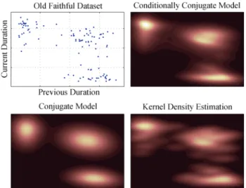
We use the duration of consecutive eruptions of the Old Faithful geyser[20] as a two dimensional example. The three dimensional Spiral dataset used in [11], the four dimensional “Iris” dataset used in [21] and the 13 dimensional “Wine” dataset[22] are modeled for assess-ing the model performance and the computational cost in higher dimensions.
The density of each dataset has been estimated using the conjugate model (CDP), the three different sam-pling schemes for the conditionally conjugate model (CCDP),SampleBoth, SampleMu, and SampleS, and by kernel density estimation③ (KDE) using Gaussian kernels.
5.1 Density Estimation Performance
As a measure for modeling performance, we use the average leave one out predictive densities. That is, for all datasets considered, we leave out one observation, model the density using all others, and calculate the log predictive density on the left-out datapoint. We re-peat this for all datapoints in the training set and report the average log predictive density. We choose this as a performance measure because the log predictive den-sity gives a quantity proportional to the KL divergence which is a measure of the discrepancy between the ac-tual generating density and the modeled density. The three different sampling schemes for the conditionally conjugate model all have identical equilibrium distribu-tions, therefore the result of the conditionally conjugate model is presented only once, instead of discriminating between different schemes when the predictive densities are considered.
We use the Old Faithful geyser dataset to visu-alise the estimated densities, Fig.3. Visualisation is important for giving an intuition about the behaviour of the different algorithms. Convergence and mixing of all samplers is fast for the two dimensional Geyser dataset. There is also not a significant difference in the predictive performance, see Tables 1 and 2. How-ever, we can see form the plots in Fig.3 and the average entropy values in Table 3 that the resulting density esti-mates are different for all models. CDP uses fewer com-ponents to fit the data, therefore the density estimate has fewer modes compared to the estimates obtained by CCDP or KDE. In Fig.3 we see three almost Gaus-sian modes for CDP. Since KDE places a kernel on each datapoint, its resulting density estimate is less smooth. Note that both CDP and CCDP have the potential to use one component per datapoint and return the same estimate as the KDE, however their prior as well as the
likelihood of the data does not favor this. The density fit by CCDP can be seen as an interpolation between the CDP and the KDE results as it utilizes more mix-ture components than CDP but has a smoother density estimate than KDE. For all datasets, the KDE model has the lowest average leave one out predictive density, and the conditionally conjugate model has the best, with the difference between the models getting larger in higher dimensions, see Table 1. For instance, on the Wine data CCDP is five fold better than KDE.
Fig.3. Old Faithful geyser dataset and its density modelled by CDP, CCDP and KDE. The two dimensional data consists of the durations of the consecutive eruptions of the Old Faithful geyser.
Table 1. Average Leave One Out Log-Predictive Densi-ties for Kernel Density Estimation (KDE), Conjugate DP Mixture Model (CDP), Conditionally Conjugate DP Mixture Model (CCDP) on Different Datasets
Dataset KDE CDP CCDP
Geyser −1.906 −1.902 −1.879 Spiral −7.205 −7.123 −7.117 Iris −1.860 −1.577 −1.546 Wine −18.979 −17.595 −17.341
Table 2. Pairedt-Test Scores of Leave One Out Predictive Densities (The test does not give enough evidence in case of the Geyser data, however it shows that KDE is statistically significantly different from both DP models for the higher di-mensional datasets. Also, CDP is significantly different from CCDP for the Wine data.)
Dataset KDE/CDP KDE/CCDP CDP/CCDP
Geyser 0.95 0.59 0.41
Spiral <0.01 <0.01 0.036 Iris <0.01 <0.01 0.099 Wine <0.01 <0.01 <0.01
③Kernel density estimation is a classical non parametric density estimation technique which places kernels on each training
data-point. The kernel bandwidth is adjusted separately on each dimension to obtain a smooth density estimate, by maximising the sum of leave-one-out log densities.
p-values for a paired t-test are given in Table 2 to compare the distribution of the leave one out densities. There is no statistically significant difference between any of the models on the Geyser dataset. For the Spi-ral, Iris and Wine datasets, the difference between the predictions of KDE and both DP models are statisti-cally significant. CCDP is significantly different from CDP in terms of its predictive density only on the Wine dataset.
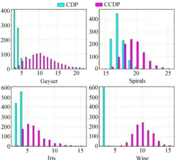
Furthermore, for all datasets, the CCDP consistently utilizes more components than CDP. The average num-ber of datapoints assigned to different components and the distribution over the number of active components are given in Fig.4 and Fig.5, respectively. Fig.5 shows that the distribution of the number of components used by the CCDP is much broader and centered on higher
Fig.4. Number of datapoints assigned to the components aver-aged over different positions in the chain. The standard devia-tions are indicated by the error bars. Note the existence of many small components for the CCDP model.
Table 3. Average Entropies of Mixing Proportions for the Conjugate DP Mixture Model (CDP), Conditionally Conju-gate DP Mixture Model (CCDP) on Various Datasets
Dataset CDP CCDP
Geyser 1.64 (0.14) 2.65 (0.51) Spiral 4.03 (0.06) 4.10 (0.08)
Iris 1.71 (0.13) 2.13 (0.28)
Wine 1.58 (0.004) 2.35 (0.17)
Fig.5. Distribution of number of active components for DPGMM from 1000 iterations. The CDP model favors a lower number of components for all datasets. The average number of components for the CCDP model is larger, with a more diffuse distribution. Note that histogram for the CDP model for the Geyser dataset and the Wine dataset has been cut off on they-axis.
values. The difference in the density estimates is also reflected in the average entropy values reported in Ta-ble 3.
5.2 Clustering Performance
The main objective of the models presented in this paper is density estimation, but the models can be used for clustering (or classification where labels are avail-able) as well by observing the assignment of datapoints to model components. Since the number of components change over the chain, one would need to form a con-fusion matrix showing the frequency of each data pair being assigned to the same component for the entire Markov chain, see Fig.6.
Class labels are available for the Iris and Wine datasets, both datasets consisting of 3 classes. The CDP model has 3∼4 active components for the Iris data and 3 active components for the Wine dataset. The assignment of datapoints to the components shows suc-cessful clustering. The CCDP model has more compo-nents on average for both datasets, but datapoints with different labels are generally not assigned to the same component, resulting in successful clustering which can be seen by the block diagonal structure of the confu-sion matrices given in Fig.6, and comparing to the true labels given on the right hand side figures. The confu-sion matrices were constructed by counting the number of times each datapoint was assigned to the same com-ponent with another datapoint. Note that the CCDP utilizes more clusters, resulting in less extreme values
Fig.6. Confusion matrices for the Iris dataset: (a) CDP; (b) CCDP; (c) Correct labels. Wine dataset: (d) CDP; (e) CCDP; (f) Correct labels. Brighter means higher, hence the darker gray values for the datapoints that were not always assigned to the same component. for the confusion matrix entries (darker gray values of
the confusion matrix) which expresses the uncertainty in cluster assignments for some datapoints. Further-more, we can see in Fig.6(d) that there is one datapoint in the Wine dataset that CDP assigns to the wrong cluster for almost all MCMC iterations, whereas this datapoint is allowed to have its own cluster by CCDP. The Spiral dataset is generated by sampling 5 points form each of the 160 Gaussians whose means lie on a spiral. For this data, the number of active components of CDP and CCDP do not go beyond 21 and 28, respec-tively. This is due to the assumption of independence of component means for both models, which does not hold for this dataset, therefore it is not surprising that the models do not find the correct clustering structure although they can closely estimate the density.
5.3 Computational Cost
The differences in density estimates and predictive performances show that different specification of the base distribution leads to different behaviour of the model on the same data. It is also interesting to find out if there is a significant gain (if at all) in compu-tational efficiency when conjugate base distribution is used rather than the non-conjugate one. The inference algorithms considered only differ in the way they up-date the indicator variables, therefore the computation time per iteration is similar for all algorithms.
We use the convergence and burn-in time as mea-sures of computational cost. Convergence was deter-mined by examining various properties of the state of
the Markov chain, and mixing time was calculated as the sum of the auto-covariance coefficients of the slow-est mixing quantities from lag−1000 to 1000.
The slowest mixing quantity was the number of ac-tive components in all experiments. Example auto-covariance coefficients are shown in Fig.7. The con-vergence time for the CDP model is usually shorter than theSampleBothscheme of CCDP but longer than the two other schemes. For the CCDP model, the SampleBothscheme is the slowest in terms of both con-verging and mixing. SampleS has comparable conver-gence time to theSampleMuscheme.
6 Conclusions
The Dirichlet process mixtures of Gaussians model is one of the most widely used DPM models. We have pre-sented hierarchical formulations of DPGMM with con-jugate and conditionally concon-jugate base distributions. The only difference between the two models is the prior on µ and the related hyperparameters. We kept the specifications for all other parameters the same so as to make sure only the presence or absence of conju-gacy would effect the results. We compared the two model specifications in terms of their modeling proper-ties for density estimation and clustering and the com-putational cost of the inference algorithms on several datasets with differing dimensions.
Experiments show that the behaviour of the two base distributions differ. For density estimation, the predic-tive accuracy of the CCDP model is found to be better than the CDP model for all datasets considered, the
Fig.7. Autocorrelation coefficients of the number of active components for CDP and different sampling schemes for CCDP, for the Spiral data based on 5×10⁵iterations, the Iris data based on 106 iterations and Wine data based on 1.5×10⁶iterations.
difference being larger in high dimensions. The CDP model tends to use less components than the CCDP model, having smaller entropy. The clustering perfor-mance of both cases are comparable, with the CCDP expressing more uncertainty on some datapoints and al-lowing some datapoints to have their own cluster when they do not match the datapoints in other clusters. From the experimental results we can conclude that the more restrictive form of the base distribution forces the conjugate model to be more parsimonious in the num-ber of components utilized. This may be a desirable feature if only a rough clustering is adequate for the task in hand, however it has the risk of overlooking the outliers in the dataset and assigning them to a cluster together with other datapoints. Since it is more flexible in the number of components, the CCDP model may in general result in more reliable clusterings.
We adjusted MCMC algorithms from [9] for infer-ence on both specifications of the model and proposed two sampling schemes for the conditionally conjugate base model with improved convergence and mixing properties. Although MCMC inference on the conju-gate case is relatively easier to implement, experimental results show that it is not necessarily computationally cheaper than inference on the conditionally conjugate model when conditional conjugacy is exploited.
In the light of the empirical results, we conclude that marginalising over one of the parameters by exploiting conditional conjugacy leads to considerably faster mix-ing in the conditionally conjugate model. When usmix-ing this trick, the fully conjugate model is not necessar-ily computationally cheaper in the case of DPGMM. The DPGMM with the more flexible prior specification (conditionally conjugate prior) can be used on higher dimensional density estimation problems, resulting in better density estimates than the model with conjugate
prior specification.
References
[1] Ferguson T S. A Bayesian analysis of some nonparametric problems.Annals of Statistics, 1973, 1(2): 209-230.
[2] Blackwell D, MacQueen J B. Ferguson distributions via P´olya urn schemes. Annals of Statistics, 1973, 1(2): 353-355. [3] Aldous D. Exchangeability and Related Topics. Ecole d’´Et´e
de Probabilit´es de Saint-Flour XIII–1983, Berlin: Springer, 1985, pp.1-198.
[4] Pitman J. Combinatorial Stochastic Processes Ecole d’Et´e de Probabilit´es de Saint-Flour XXXII – 2002, Lecture Notes in Mathematics, Vol. 1875, Springer, 2006.
[5] Sethuraman J, Tiwari R C. Convergence of Dirichlet Mea-sures and the Interpretation of Their Parameter. Statistical Decision Theory and Related Topics, III, Gupta S S, Berger J O (eds.), London: Academic Press, Vol.2, 1982, pp.305-315. [6] Ishwaran H, James L F. Gibbs sampling methods for stick-breaking priors. Journal of the American Statistical Associ-ation, March 2001, 96(453): 161-173.
[7] Antoniak C E. Mixtures of Dirichlet processes with applica-tions to Bayesian nonparametric problems.Annals of Statis-tics, 1974, 2(6): 1152–1174.
[8] Neal R M. Bayesian mixture modeling. In Proc. the 11th International Workshop on Maximum Entropy and Bayesian Methods of Statistical Analysis, Seattle, USA, June, 1991, pp.197-211.
[9] Neal R M. Markov chain sampling methods for Dirichlet pro-cess mixture models. Journal of Computational and Graphi-cal Statistics, 2000, 9(2): 249-265.
[10] Green P, Richardson S. Modelling heterogeneity with and without the Dirichlet process. Scandinavian Journal of Statistics, 2001, 28: 355-375.
[11] Rasmussen C E. The infinite Gaussian mixture model. Ad-vances in Neural Information Processing Systems, 2000, 12: 554-560.
[12] Escobar M D. Estimating normal means with a Dirichlet pro-cess prior. Journal of the American Statistical Association, 1994, 89(425): 268-277.
[13] MacEachern S N. Estimating normal means with a conjugate style Dirichlet process prior. Communications in Statistics: Simulation and Computation, 1994, 23(3): 727-741.
[14] Escobar M D, West M. Bayesian density estimation and in-ference using mixtures. Journal of the American Statistical
Association, 1995, 90(430): 577-588.
[15] M¨uller P, Erkanli A, West M. Bayesian curve fitting using multivariate normal mixtures. Biometrika, 1996, 83(1): 67-79.
[16] West M, M¨uller P, Escobar M D. Hierarchical Priors and Mix-ture Models with Applications in Regression and Density Es-timation. Aspects of Uncertainty, Freeman P R, Smith A F M (eds.), John Wiley, 1994, pp.363-386.
[17] MacEachern S N, M¨uller P. Estimating mixture of Dirich-let process models.Journal of Computational and Graphical Statistics, 1998, 7(2): 223-238.
[18] Neal R M. Markov chain sampling methods for Dirichlet pro-cess mixture models. Technical Report 4915, Department of Statistics, University of Toronto, 1998.
[19] Gilks W R, Wild P. Adaptive rejection sampling for Gibbs sampling. Applied Statistics, 1992, 41(2): 337-348.
[20] Scott D W. Multivariate Density Estimation: Theory, Prac-tice and Visualization, Wiley, 1992.
[21] Fisher R A. The use of multiple measurements in axonomic problems.Annals of Eugenics, 1936, 7: 179-188.
[22] Forina M, Armanino C, Castino M, Ubigli M. Multivariate data analysis as a discriminating method of the origin of wines.Vitis, 1986, 25(3): 189-201.
Dilan G¨or¨ur is a post-doctoral research fellow in the Gatsby Com-putational Neuroscience Unit, Uni-versity College London. She com-pleted her Ph.D. on machine learn-ing in 2007 at the Max Planck Insti-tute for Biological Cybernetics, Ger-many under the supervision of Carl Edward Rasmussen. She received the B.S. and M.Sc. degrees from Electri-cal and Electronics Engineering Department of Middle East Technical University, Turkey in 2000 and 2003, respectively. Her research interests lie in the theoretical and practical as-pects of machine learning and Bayesian inference.
Carl Edward Rasmussen is a lecturer in the Computational and Biological Learning Lab at the De-partment of Engineering, University of Cambridge and an adjunct re-search scientist at the Max Planck Institute for Biological Cybernetics, T¨ubingen, Germany. His main re-search interests are Bayesian infer-ence and machine learning. He re-ceived his Masters’ degree in engineering from the Techni-cal University of Denmark and his Ph.D. degree in com-puter science from the University of Toronto in 1996. Since then he has been a post doc at the Technical University of Denmark, a senior research fellow at the Gatsby Computa-tional Neuroscience Unit at University College London from 2000 to 2002 and a junior research group leader at the Max Planck Institute for Biological Cybernetics in T¨ubingen, Germany, form 2002 to 2007.