A PDF version is available at http://www.bottomupcs.com/csbu.pdf. The original souces are available at https:// github.com/ianw/bottomupcs
Copyright © 2004, 2005, 2006, 2007, 2008, 2009, 2010, 2011, 2012, 2013 Ian Wienand
Abstract
Computer Science from the Bottom Up — A free, online book designed to teach computer science from the bottom end up. Topics covered include binary and binary logic, operating systems internals, toolchain fundamentals and system library fundamentals.
This work is licensed under the Creative Commons Attribution-ShareAlike License. To view a copy of this license, visit http://creativecommons.org/ licenses/by-sa/3.0/ or send a letter to Creative Commons, 559 Nathan Abbott Way, Stanford, California 94305, USA.
Introduction ... xi
Welcome ... xi
Philosophy ... xi
Why from the bottom up? ... xi
Enabling technologies ... xi
1. General Unix and Advanced C ... 1
Everything is a file! ... 1
Implementing abstraction ... 2
Implementing abstraction with C ... 2
Libraries ... 4
File Descriptors ... 5
The Shell ... 8
2. Binary and Number Representation ... 11
Binary -- the basis of computing ... 11
Binary Theory ... 11
Hexadecimal ... 16
Practical Implications ... 17
Types and Number Representation ... 19
C Standards ... 19
Types ... 20
Number Representation ... 25
3. Computer Architecture ... 33
The CPU ... 33
Branching ... 33
Cycles ... 34
Fetch, Decode, Execute, Store ... 34
CISC v RISC ... 37
Memory ... 38
Memory Hierarchy ... 38
Cache in depth ... 39
Peripherals and busses ... 42
Peripheral Bus concepts ... 42
DMA ... 44
Other Busses ... 45
Small to big systems ... 46
Symmetric Multi-Processing ... 46
Clusters ... 48
Non-Uniform Memory Access ... 49
Memory ordering, locking and atomic operations ... 51
4. The Operating System ... 56
The role of the operating system ... 56
Abstraction of hardware ... 56
Multitasking ... 56
Standardised Interfaces ... 56
Security ... 57
Performance ... 57
Operating System Organisation ... 57
The Kernel ... 58
Userspace ... 61
System Calls ... 62
Analysing a system call ... 62
Privileges ... 69
Hardware ... 69
Other ways of communicating with the kernel ... 74
File Systems ... 74
5. The Process ... 75
What is a process? ... 75
Elements of a process ... 76
Process ID ... 77
Memory ... 77
File Descriptors ... 82
Registers ... 82
Kernel State ... 82
Process Hierarchy ... 83
Fork and Exec ... 83
Fork ... 83
Exec ... 84
How Linux actually handles fork and exec ... 84
The init process ... 86
Context Switching ... 88
Scheduling ... 88
Preemptive v co-operative scheduling ... 88
Realtime ... 88
Nice value ... 89
A brief look at the Linux Scheduler ... 89
The Shell ... 90
Signals ... 90
Example ... 91
6. Virtual Memory ... 93
What Virtual Memory isn't ... 93
What virtual memory is ... 93
64 bit computing ... 93
Using the address space ... 94
Pages ... 94
Physical Memory ... 95
Pages + Frames = Page Tables ... 95
Virtual Addresses ... 95
Page ... 96
Offset ... 96
Virtual Address Translation ... 96
Consequences of virtual addresses, pages and page tables ... 97
Individual address spaces ... 97
Protection ... 98
Swap ... 98
Sharing memory ... 99
Disk Cache ... 99
Hardware Support ... 99
Physical v Virtual Mode ... 99
The TLB ... 101
TLB Management ... 102
Linux Specifics ... 103
Address Space Layout ... 103
Three Level Page Table ... 104
x86-64 ... 106
Itanium ... 106
7. The Toolchain ... 113
Compiled v Interpreted Programs ... 113
Compiled Programs ... 113
Interpreted programs ... 113
Building an executable ... 113
Compiling ... 114
The process of compiling ... 114
Syntax ... 114
Assembly Generation ... 114
Optimisation ... 119
Assembler ... 120
Linker ... 120
Symbols ... 120
The linking process ... 121
A practical example ... 121
Compiling ... 122
Assembly ... 124
Linking ... 125
The Executable ... 126
8. Behind the process ... 130
Review of executable files ... 130
Representing executable files ... 130
Three Standard Sections ... 130
Binary Format ... 130
Binary Format History ... 130
ELF ... 131
ELF in depth ... 131
Debugging ... 140
ELF Executables ... 145
Libraries ... 146
Static Libraries ... 146
Shared Libraries ... 148
ABI's ... 148
Byte Order ... 148
Calling Conventions ... 148
Starting a process ... 149
Kernel communication to programs ... 149
Starting the program ... 150
9. Dynamic Linking ... 155
Code Sharing ... 155
Dynamic Library Details ... 155
Including libraries in an executable ... 155
The Dynamic Linker ... 157
Relocations ... 157
Position Independence ... 159
Global Offset Tables ... 159
The Global Offset Table ... 160
Libraries ... 164
The Procedure Lookup Table ... 164
Working with libraries and the linker ... 171
Library versions ... 171
10. I/O Fundamentals ... 181
File System Fundamentals ... 181
Networking Fundamentals ... 181
1.1. Abstraction ... 2
1.2. Default Unix Files ... 6
1.3. Abstraction ... 7
1.4. A pipe in action ... 9
2.1. Masking ... 18
2.2. Types ... 21
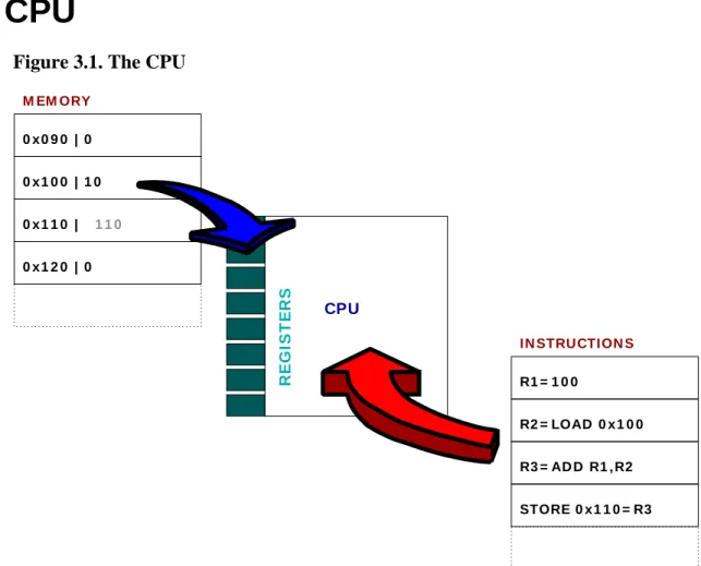
3.1. The CPU ... 33
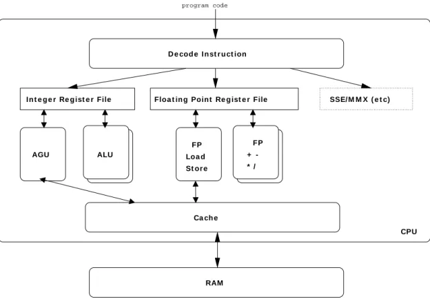
3.2. Inside the CPU ... 35
3.3. Reorder buffer example ... 36
3.4. Cache Associativity ... 40
3.5. Cache tags ... 41
3.6. Overview of handling an interrupt ... 43
3.7. Overview of a UHCI controller operation ... 45
3.8. A Hypercube ... 50
3.9. Acquire and Release semantics ... 53
4.1. The Operating System ... 58
4.2. The Operating System ... 60
4.3. Rings ... 70
4.4. x86 Segmentation Adressing ... 72
4.5. x86 segments ... 73
5.1. The Elements of a Process ... 76
5.2. The Stack ... 78
5.3. Process memory layout ... 81
5.4. Threads ... 85
5.5. The O(1) scheduler ... 89
6.1. Illustration of canonical addresses ... 94
6.2. Virtual memory pages ... 95
6.3. Virtual Address Translation ... 97
6.4. Segmentation ... 100
6.5. Linux address space layout ... 104
6.6. Linux Three Level Page Table ... 105
6.7. Illustration Itanium regions and protection keys ... 106
6.8. Illustration of Itanium TLB translation ... 107
6.9. Illustration of a hierarchical page-table ... 109
6.10. Itanium short-format VHPT implementation ... 110
6.11. Itanium PTE entry formats ... 111
7.1. Alignment ... 115
7.2. Alignment ... 116
8.1. ELF Overview ... 132
9.1. Memory access via the GOT ... 161
1.1. Standard Files Provided by Unix ... 5
1.2. Standard Shell Redirection Facilities ... 8
2.1. Binary ... 11
2.2. 203 in base 10 ... 11
2.3. 203 in base 2 ... 11
2.4. Convert 203 to binary ... 12
2.5. Bytes ... 13
2.6. Truth table for not ... 14
2.7. Truth table for and ... 14
2.8. Truth table for or ... 15
2.9. Truth table for xor ... 15
2.10. Boolean operations in C ... 16
2.11. Hexadecimal, Binary and Decimal ... 16
2.12. Convert 203 to hexadecimal ... 17
2.13. Standard Integer Types and Sizes ... 22
2.14. Standard Scalar Types and Sizes ... 22
2.15. One's Complement Addition ... 25
2.16. Two's Complement Addition ... 26
2.17. IEEE Floating Point ... 27
2.18. Scientific Notation for 1.98765x10^6 ... 27
2.19. Significands in binary ... 27
2.20. Example of normalising 0.375 ... 28
3.1. Memory Hierarchy ... 38
9.1. Relocation Example ... 158
1.1. Abstraction with function pointers ... 2
1.2. Abstraction in include/linux/virtio.h ... 4
1.3. Example of major and minor numbers ... 7
2.1. Using flags ... 18
2.2. Example of warnings when types are not matched ... 24
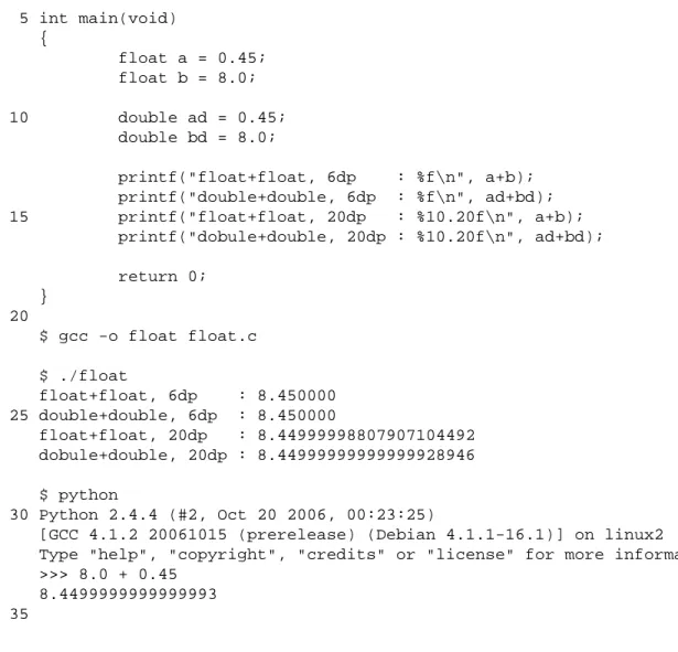
2.3. Floats versus Doubles ... 27
2.4. Program to find first set bit ... 29
2.5. Examining Floats ... 30
2.6. Analysis of 8.45 ... 32
3.1. Memory Ordering ... 52
4.1. getpid() example ... 63
4.2. PowerPC system call example ... 63
4.3. x86 system call example ... 67
5.1. Stack pointer example ... 79
5.2. pstree example ... 83
5.3. Zombie example process ... 87
5.4. Signals Example ... 91
7.1. Struct padding example ... 116
7.2. Stack alignment example ... 117
7.3. Page alignment manipulations ... 118
7.4. Hello World ... 122
7.5. Function Example ... 122
7.6. Compilation Example ... 122
7.7. Assembly Example ... 124
7.8. Readelf Example ... 124
7.9. Linking Example ... 125
7.10. Executable Example ... 126
8.1. The ELF Header ... 133
8.2. The ELF Header, as shown by readelf ... 133
8.3. Inspecting the ELF magic number ... 134
8.4. Investigating the entry point ... 134
8.5. The Program Header ... 135
8.6. Sections ... 136
8.7. Sections ... 137
8.8. Sections readelf output ... 137
8.9. Sections and Segments ... 139
8.10. Example of creating a core dump and using it with gdb™ ... 140
8.11. Example of stripping debugging information into separate files using objcopy™ ... 141
8.12. Example of using readelf™ and eu-readelf™ to examine a coredump. ... 142
8.13. Segments of an executable file ... 145
8.14. Creating and using a static library ... 146
8.15. Disassembley of program startup ... 150
8.16. Constructors and Destructors ... 152
9.1. Specifying Dynamic Libraries ... 156
9.2. Looking at dynamic libraries ... 156
9.3. Checking the program interpreter ... 157
9.4. Relocation as defined by ELF ... 158
9.5. Specifying Dynamic Libraries ... 159
9.6. Using the GOT ... 161
9.7. Relocations against the GOT ... 163
9.9. Hello world main() ... 165
9.10. Hello world sections ... 165
9.11. Hello world PLT ... 167
9.12. Hello world GOT ... 168
9.13. Dynamic Segment ... 169
9.14. Code in the dynamic linker for setting up special values (from libc sysdeps/ia64/dl-machine.h) ... 170
9.15. Symbol definition from ELF ... 174
9.16. Examples of symbol bindings ... 175
9.17. Example of LD_PRELOAD ... 177
Welcome
Welcome to Computer Science from the Bottom Up
Philosophy
In a nutshell, what you are reading is intended to be a shop class for computer science. Young computer science students are taught to "drive" the computer; but where do you go to learn what is under the hood? Trying to understand the operating system is unfortunately not as easy as just opening the bonnet. The current Linux kernel runs into the millions of lines of code, add to that the other critical parts of a modern operating system (the compiler, assembler and system libraries) and your code base becomes unimaginable. Further still, add a University level operating systems course (or four), some good reference manuals, two or three years of C experience and, just maybe, you might be able to figure out where to
start looking to make sense of it all.
To keep with the car analogy, the prospective student is starting out trying to work on a Forumla One engine without ever knowing how a two stroke motor operates. During their shop class the student should pull apart, twist, turn and put back together that two stroke motor, and consequentially have a pretty good framework for understanding just how the Formula One engine works. Nobody will expect them to be a Formula One engineer, but they are well on their way!
Why from the bottom up?
Not everyone wants to attend shop class. Most people only want to drive the car, not know how to build one from scratch. Obviously any general computing curriculum has to take this into account else it won't be relevant to its students. So computer science is taught from the "top down"; applications, high level programming, software design and development theory, possibly data structures. Students will probably be exposed to binary, hopefully binary logic, possibly even some low level concepts such as registers, opcodes and the like at a superficial level.
This book aims to move in completely the opposite direction, working from operating systems fundamentals through to how those applications are complied and executed.
Enabling technologies
This book is only possible thanks to the development of Open Source technologies. Before Linux it was like taking a shop course with a car that had it's bonnet welded shut; today we are in a position to open that bonnet, poke around with the insides and, better still, take that engine and use it to do whatever we want.
C
Everything is a file!
An often quoted tenet of UNIX-like systems such as Linux or BSD is everything is a file.
Imagine a file in the context something familiar like a word processor. There are two fundamental operations we could use on this imaginary word processing file:
1. Read it (existing saved data from the word processor). 2. Write to it (new data from the user).
Consider some of the common things attached to a computer and how they relate to our fundamental file operations:
1. The screen 2. The keyboard 3. A printer 4. A CDROM
The screen and printer are both like a write-only file, but instead of being stored as bits on a disk the information is displayed as dots on a screen or lines on a page. The keyboard is like a read only file, with the data coming from keystrokes provided by the user. The CDROM is similar, but rather than randomly coming from the user the data is stored directly on the disk.
Thus the concept of a file is a good abstraction of either a a sink for, or source of, data. As such it is an excellent abstraction of all the devices one might attach to the computer. This realisation is the great power of UNIX and is evident across the design of the entire platform. It is one of the fundamental roles of the operating system to provide this abstraction of the hardware to the programmer.
It is probably not too much of a strech to say abstraction is the primary concept that underpins all modern computing. No one person can understand everythinig from designing a modern user-interface to the internal workings of a modern CPU, much less build it all themselves. To programmers, abstractions are the lingua franca that allows us to collaborate and invent.
Learning to navigate across abstractions gives one greater insight into how to use the abstractions in the best and most innovative ways. In this book, we are concerned with abstractions at the lowest layers; bewteen applications and the operating-system and the operating-system and hardware. Above this lies many more layers, each worthy of their own books. As these chapters progress, you will hopefully gain some insight into the abstractions presented by a modern operating-system.
Figure 1.1. Abstraction
Sp ot t h e d if f e r e n ce ?
Implementing abstraction
In general, abstraction is implemented by what is generically termed an Application Programming
Interface (API). API is a somewhat nebulous term that means different things in the context of various
programming endavours. Fundamentally, a programmer designs a set of functions and documents their interface and functionality with the principle that the actual implementation providing the API is opaque. For example, many large web-applications provide an API accessible via HTTP. Accessing data via this method surely triggers many complicated series of remote-procedure calls, database queries and data transfer; all of which is opaque to the end user who simply receives the contracted data.
Those familiar with object-oriented languages such as Java, Python or C++ would be familiar with the abstraction provided by classes. Methods provide the interface to the class, but abstract the implementation.
Implementing abstraction with C
A common method used in the Linux Kernel and other large C code bases, which lacks a built-in concept of object-orientation, is function pointers. Learning to read this idom is key to navigating most large C code-bases. By understanding how to read the abstractions provided within the code an understanding of internal API designs can be built.
Example 1.1. Abstraction with function pointers
#include <stdio.h>
/* The API to implement */ struct greet_api
{
int (*say_hello)(char *name); int (*say_goodbye)(void); };
int say_hello_fn(char *name) {
printf("Hello %s\n", name); return 0;
}
/* Our implementation of the goodbye function */ int say_goodbye_fn(void)
{
printf("Goodbye\n"); return 0;
}
/* A struct implementing the API */ struct greet_api greet_api =
{
.say_hello = say_hello_fn, .say_goodbye = say_goodbye_fn };
/* main() doesn't need to know anything about how the * say_hello/goodbye works, it just knows that it does */ int main(int argc, char *argv[])
{
greet_api.say_hello(argv[1]); greet_api.say_goodbye();
printf("%p, %p, %p\n", greet_api.say_hello, say_hello_fn, &say_hello_fn); exit(0);
}
Code such as the above is the simplest example of constructs used repeatedly through the Linux Kernel and other C programs. Lets have a look at some specific elements.
We start out with a structure that defines the API (struct greet_api). The functions whose names are encased in parenthesis with a pointer marker describe a function pointer1. The function pointer describes the prototype of function it must point to; pointing it at a function without the correct return type or parameters will generate a compiler warning at least; if left in code will likely lead to incorrect operation or crashes.
We then have our implementation of the API. Often for more complex functionality you will see an idiom where API implementation functions will only be a wrapper around another function that is conventionally prepended with one or or two underscores2 (i.e. say_hello_fn() would call another function _say_hello_function()). This has several uses; generally it relates to having simpler and smaller parts of the API (marshalling or checking arguments, for example) separate to more complex implemenation, which often eases the path to significant changes in the internal workings whilst ensuring the API remains constant. Our implementation is very simple however, and doesn't even need it's own support functions. In various projects, single, double or even triple underscore function prefixes will mean different things, but universally it is a visual warning that the function is not supposed to be called directly from "beyond" the API.
1
Often you will see that the names of the parameters are omitted, and only the type of the parameter is specified. This allows the implementer to specify their own parameter names avoiding warnings from the compiler.
Second to last, we fill out the function pointers in struct greet_api greet_api. The name of the function is a pointer, therefore there is no need to take the address of the function (i.e. &say_hello_fn). Finally we can call the API functions through the structure in main.
You will see this idiom constantly when navigating the souce code. The tiny example below is taken from
include/linux/virtio.h in the Linux kernel source to illustrate:
Example 1.2. Abstraction in
include/linux/virtio.h
/**
* virtio_driver - operations for a virtio I/O driver
* @driver: underlying device driver (populate name and owner). * @id_table: the ids serviced by this driver.
* @feature_table: an array of feature numbers supported by this driver. * @feature_table_size: number of entries in the feature table array.
* @probe: the function to call when a device is found. Returns 0 or -errno. * @remove: the function to call when a device is removed.
* @config_changed: optional function to call when the device configuration * changes; may be called in interrupt context.
*/
struct virtio_driver {
struct device_driver driver;
const struct virtio_device_id *id_table; const unsigned int *feature_table;
unsigned int feature_table_size;
int (*probe)(struct virtio_device *dev); void (*scan)(struct virtio_device *dev); void (*remove)(struct virtio_device *dev);
void (*config_changed)(struct virtio_device *dev); #ifdef CONFIG_PM
int (*freeze)(struct virtio_device *dev); int (*restore)(struct virtio_device *dev); #endif
};
It's only necessary to vaguely understand that this structure is a description of a virtual I/O device. We can see the user of this API (the device driver author) is expected to provide a number of functions that will be called under various conditions during system operation (when probing for new hardware, when hardware is removed, etc). It also contains a range of data; structures which should be filled with relevant data. Starting with descriptors like this is usually the easiest way into understanding the various layers of kernel code.
Libraries
Libraries have two roles which illustrate abstraction. • Allow programmers to reuse commonly accessed code.
• Act as a black box implementing functionality for the programmer.
For example, a library implementing access to the raw data in JPEG files has both the advantage that the many programs who wish to access image files can all use the same library and the programmers building
these programs do not need to worry about the exact details of the JPEG file format, but can concentrate their efforts on what their program wants to do with the image.
The standard library of a UNIX platform is generically referred to as libc. It provides the basic interface to the system: fundamental calls such as read(), write() and printf(). This API is described in its entirety by a specification called POSIX. It is freely available online and describes the many calls that make up the standard UNIX API.
Most UNIX platforms broadly follow the POSIX standard, though often differ small but sometimes important ways (hence the complexity of the various GNU autotools, which often tries to abstract away these differences for you). Linux has many interfaces that are not specified by POSIX; writing applications that use them exclusively will make your application less portable.
Libraries are a fundamental abstraction with many details. Later chapters will describe how libraries work in much greater detail.
File Descriptors
One of the first things a UNIX programmer learns is that every running program starts with three files already opened:
Table 1.1. Standard Files Provided by Unix
Descriptive Name File Number Description
Standard In 0 Input from the keyboard
Standard Out 1 Output to the console
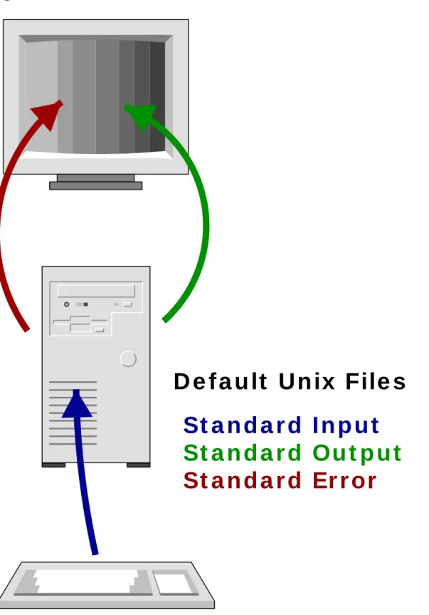
Figure 1.2. Default Unix Files
St a n d a r d I n p u t
St a n d a r d Ou t p u t
St a n d a r d Er r or
D e f a u lt Un ix File s
This raises the question what an open file represents. The value returned by an open call is termed a file
Figure 1.3. Abstraction
device_read() device_write()
device_read() device_write()
device_read() device_write() D e v ice D r iv e r s
0
1
2 3
MAX_FD
D e v ice La y e r
/dev/input
/dev/tty
/dev/sr0 Opening t he file
associat es a descript or w it h t he associat ed device
int fd = open("/dev/sr0");
w it h t he kernel w hich gives t hem a file Devices regist er
int ret = read(fd, &input, count);
File D e scr ip t or s
1
2
Furt her references t o t he descript or are rout ed t o t he device
3
File descriptors are an index into a descriptor table stored by the kernel. The kernel creates a file-descriptor in response to an open call and associates the file-descriptor with some abstraction of an underlying file-like object; be that an actual hardware device, or a file-system or something else entirely. Consequently a processes read or write calls that reference that file-descriptor are routed to the correct place by the kernel to ultimately do something useful.
In short, the file-descriptor is the gateway into the kernel's abstractions of underlying hardware. An overall view of the abstraction for physical-devices is shown in Figure 1.3, “Abstraction”.
Starting at the lowest level, the operating system requires a programmer to create a device-driver to be able to communicate with a hardware device. This device-driver is written to an API provided by the kernel just like in Example 1.2, “Abstraction in include/linux/virtio.h”; the device-driver will provide a range of functions which are called by the kernel in response to various requirements. In the simplified example above, we can see the drivers provide a read and write function that will be called in response to the analogous operations on the file-descriptor. The device-driver knows how to convert these generic requests into specific requests or commands for a particular device.
To provide the abstraction to user-space, the kernel provides a file-interface via what is generically termed a device layer. Physical devices on the host are represented by a file in a special file-system such as /dev. In UNIX-like systems, so called device-nodes have what are termed a major and a minor number which allows the kernel to associate particular nodes with their underlying driver. These can be identified via ls
as illustrated in Example 1.3, “Example of major and minor numbers”.
Example 1.3. Example of major and minor numbers
$ ls -l /dev/null /dev/zero /dev/tty
crw-rw-rw- 1 root root 5, 0 Sep 2 15:06 /dev/tty crw-rw-rw- 1 root root 1, 5 Aug 26 13:12 /dev/zero
This brings us to the file-descriptor, which is the handle user-space uses to talk to the underlying device. In a broad-sense, what happens when a file is opened is that the kernel is using the path information to map the file-descriptor with something that provides an appropriate read and write, etc. API. When this open is for a device (/dev/sr0 above), the major and minor number of the opened device-node provides the information the kernel needs to find the correct device-driver and complete the mapping. The kernel will then know how to route further calls such as read to the underlying functions provided by the device-driver.
A non-device file operates similarly, although there are more layers in-between. The abstraction here is the mount-point; mounting a file-system has the dual purpose of setting up a mapping so the file-system knows the underlying device that provides the storage and the kernel knows that files opened under that mount-point should be directed to the file-system driver. Like device-drivers, file-systems are written to a particular generic file-system API provided by the kernel.
There are indeed many other layers that complicate the picture in real-life. For example, the kernel will go to great efforts to cache as much data from disks as possible in otherwise free-memory; this provides many speed advantages. It will also try to organise device access in the most efficient ways possible; for example trying to order disk-access to ensure data stored physically close to each other is retrieved together, even if the requests did not arrive in such an order. Further, many devices are of a more generic class such as USB or SCSI devices which provide their own abstraction layers to write too. Thus rather than writing directly to devices, file-systems will go through these many layers. Understanding the kernel is to understand how these many APIs interrelate and coexist.
The Shell
The shell is the gateway to interacting with the operating system. Be it bash, zsh, csh or any of the many other shells, they all fundamentally have only one major task — to allow you to execute programs (you will begin to understand how the shell actually does this when we talk about some of the internals of the operating system later).
But shells do much more than allow you to simply execute a program. They have powerful abilities to redirect files, allow you to execute multiple programs simultaneously and script complete programs. These all come back to the everything is a file idiom.
Redirection
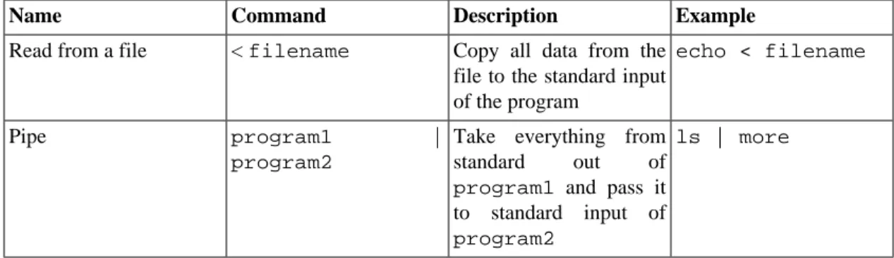
Often we do not want the standard file descriptors mentioned in the section called “File Descriptors” to point to their default places. For example, you may wish to capture all the output of a program into a file on disk, or, alternatively have it read its commands from a file you prepared earlier. Another useful task might like to pass the output of one program to the input of another. With the operating system, the shell facilitates all this and more.
Table 1.2. Standard Shell Redirection Facilities
Name Command Description Example
Redirect to a file > filename Take all output from standard out and place it into filename. Note using >> will append to the file, rather than overwrite it.
Name Command Description Example Read from a file < filename Copy all data from the
file to the standard input of the program
echo < filename
Pipe program1 | program2
Take everything from standard out of
program1 and pass it to standard input of
program2
ls | more
Implementing
pipe
The implementation of ls | more is just another example of the power of abstraction. What fundamentally happens here is that instead of associating the file-descriptor for the standard-output with some sort of underlying device (such as the console, for output to the terminal), the descriptor is pointed to an in-memory buffer provided by the kernel commonly termed a pipe. The trick here is that another process can associate its standard input with the other-side of this same buffer and effectively consume the output of the other process. This is illustrated in Figure 1.4, “A pipe in action”
Figure 1.4. A pipe in action
Bu f f e r File D e scr ip t or s
0
1
2
3
MAX_FD
File D e scr ip t or s
0
1
2
3
MAX_FD
$ ls | more
write() read() Kernel
User
p ip e
ls more
The pipe is an in-memory buffer that connects two processes together. File-descriptors point to the pipe object, which buffers data sent to it (via a write) to be drained (via a read)
Writes to the pipe are stored by the kernel until a corresponding read from the other side drains the buffer. This is a very powerful concept and is one of the fundamental forms of inter-process communication or IPC in UNIX like operating systems. The pipe allows more than just a data transfer; it can act as a signaling channel. If a process reads an empty pipe, it will by default block or be put into hibernation until there is some data available (this is discussed in much greater depth in Chapter 5, The Process. Thus two processes may use a pipe to communicate that some action has been taken just by writing a byte of data; rather than the actual data being important, the mere presence of any data in the pipe can signal a message. Say for example one process requests that another print a file - something that will take some time. The two processes may setup a pipe between themselves where the requesting process does a read
on the empty pipe; being empty that call blocks and the process does not continue. Once the print is done, the other process can write a message into the pipe, which effectively wakes up the requesting process and signals the work is done.
Allowing processes to pass data between each other like this springs another common UNIX idiom of small tools doing one particular thing. Chaining these small tools gives a flexibility that a single monolithic tool often can not.
Representation
Binary -- the basis of computing
Binary Theory
Introduction
Binary is a number system which builds numbers from elements called bits. Each bit can be represented by any two mutually exclusive states. Generally, when we write it down or code bits, we represent them with 1 and 0. We also talk about them being true and false, and the computer internally represents bits with high and low voltages.
We build binary numbers the same way we build numbers in our traditional base 10 system. However, instead of a one's column, a 10's column, a 100's column (and so on) we have a one's column, a two's columns, a four's column, an eight's column, and so on, as illustrated below.
Table 2.1. Binary
2... 26 25 24 23 22 21 20
... 64 32 16 8 4 2 1
For example, to represent the number 203 in base 10, we know we place a 3 in the 1's column, a 0 in the
10's column and a 2 in the 100's column. This is expressed with exponents in the table below.
Table 2.2. 203 in base 10
102 101 100
2 0 3
Or, in other words, 2 × 10² + 3 × 100 = 200 + 3 = 203. To represent the same thing in binary, we would have the following table.
Table 2.3. 203 in base 2
27 26 25 24 23 22 21 20
1 1 0 0 1 0 1 1
That equates to 27 + 26 + 23+21 + 20 = 128 + 64 + 8 + 2 + 1 = 203.
Conversion
The easiest way to convert between bases is to use a computer, after all, that's what they're good at! However, it is often useful to know how to do conversions by hand.
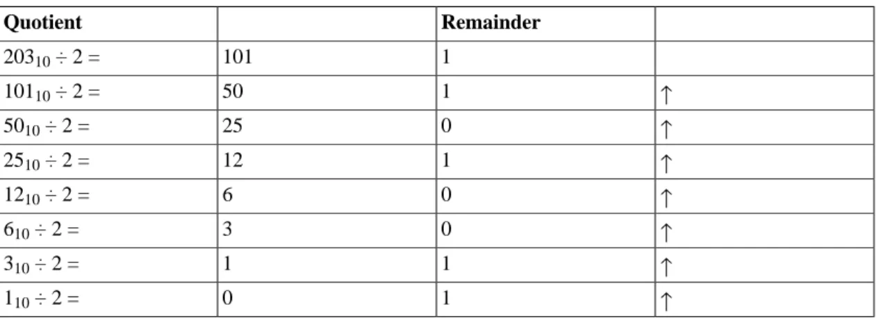
The easiest method to convert between bases is repeated division. To convert, repeatedly divide the quotient by the base, until the quotient is zero, making note of the remainders at each step. Then, write
the remainders in reverse, starting at the bottom and appending to the right each time. An example should illustrate; since we are converting to binary we use a base of 2.
Table 2.4. Convert 203 to binary
Quotient Remainder
20310 ÷ 2 = 101 1
10110 ÷ 2 = 50 1 ↑
5010 ÷ 2 = 25 0 ↑
2510 ÷ 2 = 12 1 ↑
1210 ÷ 2 = 6 0 ↑
610 ÷ 2 = 3 0 ↑
310 ÷ 2 = 1 1 ↑
110 ÷ 2 = 0 1 ↑
Reading from the bottom and appending to the right each time gives 11001011, which we saw from the previous example was 203.
Bits and Bytes
To represent all the letters of the alphabet we would need at least enough different combinations to represent all the lower case letters, the upper case letters, numbers and punctuation, plus a few extras. Adding this up means we need probably around 80 different combinations.
If we have two bits, we can represent four possible unique combinations (00 01 10 11). If we have three bits, we can represent 8 different combinations. As we saw above, with n bits we can represent 2n
unique combinations.
8 bits gives us 28 = 256 unique representations, more than enough for our alphabet combinations. We call a group of 8 bits a byte. Guess how bit a C char variable is? One byte.
ASCII
Given that a byte can represent any of the values 0 through 256, anyone could arbitrarily make up a mapping between characters and numbers. For example, a video card manufacturer could decide that the value 10 represents A, so when value 10 is sent to the video card it displays a capital 'A' on the screen.
To avoid this happening, the American Standard Code for Information Interchange or ASCII was invented. This is a 7-bit code, meaning there are 27 or 128 available codes.
The range of codes is divided up into two major parts; the non-printable and the printable. Printable characters are things like characters (upper and lower case), numbers and punctuation. Non-printable codes are for control, and do things like make a carriage-return, ring the terminal bell or the special NULL code which represents nothing at all.
127 unique characters is sufficient for American English, but becomes very restrictive when one wants to represent characters common in other languages, especially Asian languages which can have many thousands of unique characters.
To alleviate this, modern systems are moving away from ASCII to Unicode, which can use up to 4 bytes to represent a character, giving much more room!
Parity
ASCII, being only a 7-bit code, leaves one bit of the byte spare. This can be used to implement parity which is a simple form of error checking. Consider a computer using punch-cards for input, where a hole represents 1 and no hole represents 0. Any inadvertent covering of a hole will cause an incorrect value to be read, causing undefined behaviour.
Parity allows a simple check of the bits of a byte to ensure they were read correctly. We can implement either odd or even parity by using the extra bit as a parity bit.
In odd parity, if the number of 1's in the 7 bits of information is odd, the parity bit is set, otherwise it is not set. Even parity is the opposite; if the number of 1's is even the parity bit is set to 1.
In this way, the flipping of one bit will case a parity error, which can be detected. XXX more about error correcting
16, 32 and 64 bit computers
Numbers do not fit into bytes; hopefully your bank balance in dollars will need more range than can fit into one byte! Most modern architectures are 32 bit computers. This means they work with 4 bytes at a time when processing and reading or writing to memory. We refer to 4 bytes as a word; this is analogous to language where letters (bits) make up words in a sentence, except in computing every word has the same size! The size of a C it variable is 32 bits. Newer architectures are 64 bits, which doubles the size the processor works with (8 bytes).
Kilo, Mega and Giga Bytes
Computers deal with a lot of bytes; that's what makes them so powerful!
We need a way to talk about large numbers of bytes, and a natural way is to use the "International System of Units" (SI) prefixes as used in most other scientific areas. So for example, kilo refers to 103 or 1000 units, as in a kilogram has 1000 grams.
1000 is a nice round number in base 10, but in binary it is 1111101000 which is not a particularly "round" number. However, 1024 (or 210) is (10000000000), and happens to be quite close to the base ten meaning of kilo (1000 as opposed to 1024).
Hence 1024 bytes became known as a kilobyte. The first mass market computer was the Commodore 64, so named because it had 64 kilobytes of storage.
Today, kilobytes of memory would be small for a wrist watch, let alone a personal computer. The next SI unit is "mega" for 106. As it happens, 220 is again close to the SI base 10 definition; 1048576 as opposed to 1000000.
The units keep increasing by powers of 10; each time it diverges further from the base SI meaning.
Table 2.5. Bytes
210 Kilobyte
220 Megabyte
230 Gigabyte
240 Terrabyte
260 Exabyte
Therefore a 32 bit computer can address up to four gigabytes of memory; the extra two bits can represent four groups of 230 bytes.. A 64 bit computer can address up to 8 exabytes; you might be interested in working out just how big a number this is! To get a feel for how bit that number is, calculate how long it would take to count to 264 if you incremented once per second.
Kilo, Mega and Giga Bits
Apart from the confusion related to the overloading of SI units between binary and base 10, capacities will often be quoted in terms of bits rather than bytes.
Generally this happens when talking about networking or storage devices; you may have noticed that your ADSL connection is described as something like 1500 kilobits/second. The calculation is simple; multiply by 1000 (for the kilo), divide by 8 to get bytes and then 1024 to get kilobytes (so 1500 kilobits/s=183 kilobytes per second).
The SI standardisation body has recognised these dual uses, and has specified unique prefixes for binary usage. Under the standard 1024 bytes is a kibibyte, short for kilo binary byte (shortened to KiB). The other prefixes have a similar prefix (Mebibyte, for example). Tradition largely prevents use of these terms, but you may seem them in some literature.
Boolean Operations
George Boole was a mathematician who discovered a whole area of mathematics called Boolean Algebra. Whilst he made his discoveries in the mid 1800's, his mathematics are the fundamentals of all computer science. Boolean algebra is a wide ranging topic, we present here only the bare minimum to get you started. Boolean operations simply take a particular input and produce a particular output following a rule. For example, the simplest boolean operation, not simply inverts the value of the input operand. Other operands usually take two inputs, and produce a single output.
The fundamental Boolean operations used in computer science are easy to remember and listed below. We represent them below with truth tables; they simply show all possible inputs and outputs. The term
true simply reflects 1 in binary.
Not
Usually represented by !, not simply inverts the value, so 0 becomes 1 and 1 becomes 0
Table 2.6. Truth table for not
Input Output
1 0
0 1
And
To remember how the and operation works think of it as "if one input and the other are true, result is true
Table 2.7. Truth table for and
Input 1 Input 2 Output
Input 1 Input 2 Output
1 0 0
0 1 0
1 1 1
Or
To remember how the or operation works think of it as "if one input or the other input is true, the result is true
Table 2.8. Truth table for or
Input 1 Input 2 Output
0 0 0
1 0 1
0 1 1
1 1 1
Exclusive Or (xor)
Exclusive or, written as xor is a special case of or where the output is true if one, and only one, of the inputs is true. This operation can surprisingly do many interesting tricks, but you will not see a lot of it in the kernel.
Table 2.9. Truth table for xor
Input 1 Input 2 Output
0 0 0
1 0 1
0 1 1
1 1 0
How computers use boolean operations
Believe it or not, essentially everything your computer does comes back to the above operations. For example, the half adder is a type of circuit made up from boolean operations that can add bits together (it is called a half adder because it does not handle carry bits). Put more half adders together, and you will start to build something that can add together long binary numbers. Add some external memory, and you have a computer.
Electronically, the boolean operations are implemented in gates made by transistors. This is why you might have heard about transistor counts and things like Moores Law. The more transistors, the more gates, the more things you can add together. To create the modern computer, there are an awful lot of gates, and an awful lot of transistors. Some of the latest Itanium processors have around 460 million transistors.
Working with binary in C
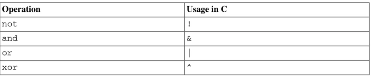
Table 2.10. Boolean operations in C
Operation Usage in C
not !
and &
or |
xor ^
We use these operations on variables to modify the bits within the variable. Before we see examples of this, first we must divert to describe hexadecimal notation.
Hexadecimal
Hexadecimal refers to a base 16 number system. We use this in computer science for only one reason, it makes it easy for humans to think about binary numbers. Computers only ever deal in binary and hexadecimal is simply a shortcut for us humans trying to work with the computer.
So why base 16? Well, the most natural choice is base 10, since we are used to thinking in base 10 from our every day number system. But base 10 does not work well with binary -- to represent 10 different elements in binary, we need four bits. Four bits, however, gives us sixteen possible combinations. So we can either take the very tricky road of trying to convert between base 10 and binary, or take the easy road and make up a base 16 number system -- hexadecimal!
Hexadecimal uses the standard base 10 numerals, but adds A B C D E F which refer to 10 11 12 13 14 15 (n.b. we start from zero).
Traditionally, any time you see a number prefixed by 0x this will denote a hexadecimal number. As mentioned, to represent 16 different patterns in binary, we would need exactly four bits. Therefore, each hexadecimal numeral represents exactly four bits. You should consider it an exercise to learn the following table off by heart.
Table 2.11. Hexadecimal, Binary and Decimal
Hexadecimal Binary Decimal
0 0000 0
1 0001 1
2 0010 2
3 0011 3
4 0100 4
5 0101 5
6 0110 6
7 0111 7
8 1000 8
9 1001 9
A 1010 10
Hexadecimal Binary Decimal
C 1100 12
D 1101 13
E 1110 14
F 1111 15
Of course there is no reason not to continue the pattern (say, assign G to the value 16), but 16 values is an excellent trade off between the vagaries of human memory and the number of bits used by a computer (occasionally you will also see base 8 used, for example for file permissions under UNIX). We simply represent larger numbers of bits with more numerals. For example, a sixteen bit variable can be represented by 0xAB12, and to find it in binary simply take each individual numeral, convert it as per the table and join them all together (so 0xAB12 ends up as the 16-bit binary number 1010101100010010). We can use the reverse to convert from binary back to hexadecimal.
We can also use the same repeated division scheme to change the base of a number. For example, to find 203 in hexadecimal
Table 2.12. Convert 203 to hexadecimal
Quotient Remainder
20310 ÷ 16 = 12 11 (0xB)
1210 ÷ 16 = 0 12 (0xC) ↑
Hence 203 in hexadecimal is 0xCB.
Practical Implications
Use of binary in code
Whilst binary is the underlying language of every computer, it is entirely practical to program a computer in high level languages without knowing the first thing about it. However, for the low level code we are interested in a few fundamental binary principles are used repeatedly.
Masking and Flags
Masking
In low level code, it is often important to keep your structures and variables as space efficient as possible. In some cases, this can involve effectively packing two (generally related) variables into one.
Remember each bit represents two states, so if we know a variable only has, say, 16 possible states it can be represented by 4 bits (i.e. 24=16 unique values). But the smallest type we can declare in C is 8 bits (a
char), so we can either waste four bits, or find some way to use those left over bits.
We can easily do this by the process of masking. Remembering the rules of the logical operations, it should become clear how the values are extracted.
The process is illustrated in the figure below. We are interested in the lower four bits, so set our mask to have these bits set to 1. Since the logical and operation will only set the bit if both bits are 1, those bits of the mask set to 0 effectively hide the bits we are not interested in.
Figure 2.1. Masking
1
1
1
1
0
0
0
0
0 x0 F
&
&
&
&
&
&
&
&
1
1
0
1
0
0
0
1
0
0
0
0
0
1
0
1
0 x0 5
To get the top (blue) four bits, we would invert the mask. You will note this gives a result of 0x90 when really we want a value of 0x09. To get the bits into the right position we use the right shift operation.
Setting the bits requires the logical or operation. However, rather than using 1's as the mask, we use 0's. You should draw a diagram similar to the above figure and work through setting bits with the
logical or operation.
Flags
Often a program will have a large number of variables that only exist as flags to some condition. For example, a state machine is an algorithm that transitions through a number of different states but may only be in one at a time. Say it has 8 different states; we could easily declare 8 different variables, one for each state. But in many cases it is better to declare one 8 bit variable and assign each bit to flag flag a particular state.
Flags are a special case of masking, but each bit represents a particular boolean state (on or off). An n bit variable can hold n different flags. See the code example below for a typical example of using flags -- you will see variations on this basic code very often.
Example 2.1. Using flags
1
#include <stdio.h>
// define all 8 possible flags for an 8 bit variable 5 // name hex binary
#define FLAG1 0x01 // 00000001 #define FLAG2 0x02 // 00000010 #define FLAG3 0x04 // 00000100 #define FLAG4 0x08 // 00001000 10 // ... and so on
#define FLAG8 0x80 // 10000000
int main(int argc, char *argv[]) {
15 char flags = 0; //an 8 bit variable
// set flags with a logical or flags = flags | FLAG1; //set flag 1 flags = flags | FLAG3; //set flag 3 20
// check flags with a logical and. If the flag is set (1) // then the logical and will return 1, causing the if // condition to be true.
if (flags & FLAG1)
25 printf("FLAG1 set!\n");
// this of course will be untrue. if (flags & FLAG8)
printf("FLAG8 set!\n"); 30
// check multiple flags by using a logical or // this will pass as FLAG1 is set
if (flags & (FLAG1|FLAG4))
printf("FLAG1 or FLAG4 set!\n"); 35
return 0; }
Types and Number Representation
C Standards
Although a slight divergence, it is important to understand a bit of history about the C language.
C is the lingua franca of the systems programming world. Every operating system and its associated system libraries in common use is written in C, and every system provides a C compiler. To stop the language diverging across each of these systems where each would be sure to make numerous incompatible changes, a strict standard has been written for the language.
Officially this standard is known as ISO/IEC 9899:1999(E), but is more commonly referred to by its shortened name C99. The standard is maintained by the International Standards Organisation (ISO) and the full standard is available for purchase online. Older standards versions such as C89 (the predecessor to C99 released in 1989) and ANSI C are no longer in common usage and are encompassed within the latest standard. The standard documentation is very technical, and details most every part of the language. For example it explains the syntax (in Backus Naur form), standard #define values and how operations should behave.
It is also important to note what the C standards does not define. Most importantly the standard needs to be appropriate for every architecture, both present and future. Consequently it takes care not to define areas that are architecture dependent. The "glue" between the C standard and the underlying architecture is the Application Binary Interface (or ABI) which we discuss below. In several places the standard will mention that a particular operation or construct has an unspecified or implementation dependent result. Obviously the programmer can not depend on these outcomes if they are to write portable code.
GNU C
The GNU C Compiler, more commonly referred to as gcc, almost completely implements the C99 standard. However it also implements a range of extensions to the standard which programmers will often use to gain extra functionality, at the expense of portability to another compiler. These extensions are usually related to very low level code and are much more common in the system programming field; the most common extension being used in this area being inline assembly code. Programmers should read the gcc documentation and understand when they may be using features that diverge from the standard.
gcc can be directed to adhere strictly to the standard (the -std=c99 flag for example) and warn or create an error when certain things are done that are not in the standard. This is obviously appropriate if you need to ensure that you can move your code easily to another compiler.
Types
As programmers, we are familiar with using variables to represent an area of memory to hold a value. In a
typed language, such as C, every variable must be declared with a type. The type tells the compiler about
what we expect to store in a variable; the compiler can then both allocate sufficient space for this usage and check that the programmer does not violate the rules of the type. In the example below, we see an example of the space allocated for some common types of variables.
Figure 2.2. Types
\0 h e l l o int a
char c
int b[2]
char *h = "hello"
1 b y t e
4 b y t e s
6 b y t e s 2 x 4 b y t e s
b[1] | *(b+1) b[0] | *b
Sy st e m M e m or y
The C99 standard purposely only mentions the smallest possible size of each of the types defined for C. This is because across different processor architectures and operating systems the best size for types can be wildly different.
To be completely safe programmers need to never assume the size of any of their variables, however a functioning system obviously needs agreements on what sizes types are going to be used in the system. Each architecture and operating system conforms to an Application Binary Interface or ABI. The ABI for a system fills in the details between the C standard and the requirements of the underlying hardware and operating system. An ABI is written for a specific processor and operating system combination.
Table 2.13. Standard Integer Types and Sizes
Type C99 minimum size (bits) Common size (32 bit architecture)
char 8 8
short 16 16
int 16 32
long 32 32
long long 64 64
Pointers Implementation dependent 32
Above we can see the only divergence from the standard is that int is commonly a 32 bit quantity, which is twice the strict minimum 16 bit size that the C99 requires.
Pointers are really just an address (i.e. their value is an address and thus "points" somewhere else in memory) therefore a pointer needs to be sufficient in size to be able to address any memory in the system.
64 bit
One area that causes confusion is the introduction of 64 bit computing. This means that the processor can handle addresses 64 bits in length (specifically the registers are 64 bits wide; a topic we discuss in Chapter 3, Computer Architecture).
This firstly means that all pointers are required to be a 64 bits wide so they can represent any possible address in the system. However, system implementors must then make decisions about the size of the other types. Two common models are widely used, as shown below.
Table 2.14. Standard Scalar Types and Sizes
Type C99 minimum size (bits)
Common size (LP64) Common size (Windows)
char 8 8 8
short 16 16 16
int 16 32 32
long 32 64 32
long long 64 64 64
Pointers Implementation dependent
64 64
You can see that in the LP64 (long-pointer 64) model long values are defined to be 64 bits wide. This is different to the 32 bit model we showed previously. The LP64 model is widely used on UNIX systems. In the other model, long remains a 32 bit value. This maintains maximum compatibility with 32 code. This model is in use with 64 bit Windows.
There are good reasons why the size of int was not increased to 64 bits in either model. Consider that if the size of int is increased to 64 bits you leave programmers no way to obtain a 32 bit variable. The only possibly is redefining shorts to be a larger 32 bit type.
A 64 bit variable is so large that it is not generally required to represent many variables. For example, loops very rarely repeat more times than would fit in a 32 bit variable (4294967296 times!). Images usually
are usually represented with 8 bits for each of a red, green and blue value and an extra 8 bits for extra (alpha channel) information; a total of 32 bits. Consequently for many cases, using a 64 bit variable will be wasting at least the top 32 bits (if not more). Not only this, but the size of an integer array has now doubled too. This means programs take up more system memory (and thus more cache; discussed in detail in Chapter 3, Computer Architecture) for no real improvement. For the same reason Windows elected to keep their long values as 32 bits; since much of the Windows API was originally written to use long variables on a 32 bit system and hence does not require the extra bits this saves considerable wasted space in the system without having to re-write all the API.
If we consider the proposed alternative where short was redefined to be a 32 bit variable; programmers working on a 64 bit system could use it for variables they know are bounded to smaller values. However, when moving back to a 32 bit system their same short variable would now be only 16 bits long, a value which is much more realistically overflowed (65536).
By making a programmer request larger variables when they know they will be needed strikes a balance with respect to portability concerns and wasting space in binaries.
Type qualifiers
The C standard also talks about some qualifiers for variable types. For example const means that a variable will never be modified from its original value and volatile suggests to the compiler that this value might change outside program execution flow so the compiler must be careful not to re-order access to it in any way.
signed and unsigned are probably the two most important qualifiers; and they say if a variable can take on a negative value or not. We examine this in more detail below.
Qualifiers are all intended to pass extra information about how the variable will be used to the compiler. This means two things; the compiler can check if you are violating your own rules (e.g. writing to a const
value) and it can make optimisations based upon the extra knowledge (examined in later chapters).
Standard Types
C99 realises that all these rules, sizes and portability concerns can become very confusing very quickly. To help, it provides a series of special types which can specify the exact properties of a variable. These are defined in <stdint.h> and have the form qtypes_t where q is a qualifier, type is the base type, s
is the width in bits and _t is an extension so you know you are using the C99 defined types.
So for example uint8_t is an unsigned integer exactly 8 bits wide. Many other types are defined; the complete list is detailed in C99 17.8 or (more cryptically) in the header file. 1
It is up to the system implementing the C99 standard to provide these types for you by mapping them to appropriate sized types on the target system; on Linux these headers are provided by the system libraries.
Types in action
Below we see an example of how types place restrictions on what operations are valid for a variable, and how the compiler can use this information to warn when variables are used in an incorrect fashion. In this code, we firstly assign an integer value into a char variable. Since the char variable is smaller, we loose the correct value of the integer. Further down, we attempt to assign a pointer to a char to memory we designated as aninteger. This operation can be done; but it is not safe. The first example is run on a
32-1Note that C99 also has portability helpers for printf. The PRI macros in <inttypes.h> can be used as specifiers for types of specified sizes.
bit Pentium machine, and the correct value is returned. However, as shown in the second example, on a 64-bit Itanium machine a pointer is 64 64-bits (8 bytes) long, but an integer is only 4 bytes long. Clearly, 8 bytes can not fit into 4! We can attempt to "fool" the compiler by casting the value before assigning it; note that in this case we have shot ourselves in the foot by doing this cast and ignoring the compiler warning since the smaller variable can not hold all the information from the pointer and we end up with an invalid address.
Example 2.2. Example of warnings when types are not matched
1
$ cat types.c #include <stdio.h>
#include <stdint.h> 5
int main(void) {
char *c; int i; 10
i = c; i = (int)c;
return 0; 15 }
$ uname -m i686
20 $ gcc -Wall -o types types.c types.c: In function 'main':
types.c:19: warning: assignment makes integer from pointer without a cast
$ ./types 25 i is 52
p is 0x80484e8 p is 0x80484e8
$ uname -m 30 ia64
$ gcc -Wall -o types types.c types.c: In function 'main':
types.c:19: warning: assignment makes integer from pointer without a cast 35 types.c:21: warning: cast from pointer to integer of different size
types.c:22: warning: cast to pointer from integer of different size
$ ./types i is 52
40 p is 0x40000000000009e0 p is 0x9e0
Number Representation
Negative Values
With our modern base 10 numeral system we indicate a negative number by placing a minus (-) sign in front of it. When using binary we need to use a different system to indicate negative numbers.
There is only one scheme in common use on modern hardware, but C99 defines three acceptable methods for negative value representation.
Sign Bit
The most straight forward method is to simply say that one bit of the number indicates either a negative or positive value depending on it being set or not.
This is analogous to mathematical approach of having a + and -. This is fairly logical, and some of the original computers did represent negative numbers in this way. But using binary numbers opens up some other possibilities which make the life of hardware designers easier.
However, notice that the value 0 now has two equivalent values; one with the sign bit set and one without. Sometimes these values are referred to as +0 and -0 respectively.
One's Complement
One's complement simply applies the not operation to the positive number to represent the negative number. So, for example the value -90 (-0x5A) is represented by ~01011010 = 101001012
With this scheme the biggest advantage is that to add a negative number to a positive number no special logic is required, except that any additional carry left over must be added back to the final value. Consider
Table 2.15. One's Complement Addition
Decimal Binary Op
-90 10100101 +
100 01100100
---
---10 100001001 9
00001010 10
If you add the bits one by one, you find you end up with a carry bit at the end (highlighted above). By adding this back to the original we end up with the correct value, 10
Again we still have the problem with two zeros being represented. Again no modern computer uses one's complement, mostly because there is a better scheme.
Two's Complement
Two's complement is just like one's complement, except the negative representation has one added to it and we discard any left over carry bit. So to continue with the example from before, -90 would be
~01011010+1=10100101+1 = 10100110.
2The ~ operator is the C language operator to apply NOT to the value. It is also occasionally called the one's complement operator, for obvious
This means there is a slightly odd symmetry in the numbers that can be represented; for example with an 8 bit integer we have 2^8 = 256 possible values; with our sign bit representation we could represent -127 thru 127 but with two's complement we can represent -127 thru 128. This is because we have removed the problem of having two zeros; consider that "negative zero" is (~00000000 +1)=(11111111+1)=00000000 (note discarded carry bit).
Table 2.16. Two's Complement Addition
Decimal Binary Op
-90 10100110 +
100 01100100
---
---10 00001010
You can see that by implementing two's complement hardware designers need only provide logic for addition circuits; subtraction can be done by two's complement negating the value to be subtracted and then adding the new value.
Similarly you could implement multiplication with repeated addition and division with repeated subtraction. Consequently two's complement can reduce all simple mathematical operations down to addition!
All modern computers use two's complement representation.
Sign-extension
Becuase of two's complement format, when increasing the size of signed value, it is important that the additional bits be sign-extended; that is, copied from the top-bit of the existing value.
For example, the value of an 32-bit int -10 would be represented in two's complement binary as
11111111111111111111111111110110. If one were to cast this to a 64-bit long long int, we would need to ensure that the additional 32-bits were set to 1 to maintain the same sign as the original. Thanks to two's complement, it is sufficient to take the top bit of the exiting value and replace all the added bits with this value. This processes is referred to as sign-extension and is usually handled by the compiler in situations as defined by the language standard, with the processor generally providing special instructions to take a value an sign-extended it to some larger value.
Floating Point
So far we have only discussed integer or whole numbers; the class of numbers that can represent decimal values is called floating point.
To create a decimal number, we require some way to represent the concept of the decimal place in binary. The most common scheme for this is known as the IEEE-754 floating point standard because the standard is published by the Institute of Electric and Electronics Engineers. The scheme is conceptually quite simple and is somewhat analogous to "scientific notation".
In scientific notation the value 123.45 might commonly be represented as 1.2345x10². We call
1.2345 the mantissa or significand, 10 is the radix and 2 is the exponent.
In the IEEE floating point model, we break up the available bits to represent the sign, mantissa and exponent of a decimal number. A decimal number is represented by sign × significand × 2^exponent. The sign bit equates to either 1 or -1. Since we are working in binary, we always have the implied radix of 2.


![Figure 2.2. Types \0helloint achar cint b[2]char *h = "hello" 1 b y t e 4 b y t e s 6 b y t e s 2 x 4 b y t e s b[1] | *(b+1)b[0] | *b Sy st e m M e m or y](https://thumb-us.123doks.com/thumbv2/123dok_us/8432214.2243341/32.918.176.763.134.835/figure-types-helloint-achar-cint-char-hello-sy.webp)