modeling genetic algorithms with interacting
particle systems
P. Del Moral∗– L. Kallel†– J. Rowe‡
Received: 27 July 2000; Revised version: 4 December 2000
Abstract
We present in this work a natural Interacting Particle System (IPS) approach for modeling and studying the asymptotic behavior of Genetic Algorithms (GAs). In this model, a population is seen as a distribution (or measure) on the search space, and the Genetic Algorithm as a measure valued dynamical system. This model allows one to apply recent convergence results from the IPS literature for studying the convergence of genetic algorithms when the size of the population tends to infinity.
We first review a number of approaches to Genetic Algorithms modeling and re-lated convergence results. We then describe a general and abstract discrete time Interacting Particle System model for GAs, and we propose a brief review of some re-cent asymptotic results about the convergence of theN-IPS approximating model (of finiteN-sized-population GAs) towards the IPS model (of infinite population GAs), including law of large number theorems, ILp-mean and exponential bounds as well as large deviations principles.
Finally, the impact of modeling Genetic Algorithms with our interacting particle system approach is detailed on different classes of generic genetic algorithms including mutation, cross-over and proportionate selection. We explore the connections between Feynman-Kac distribution flows and the simple genetic algorithm. This Feynman-Kac representation of the infinite population model is then used to develop asymptotic stability and uniform convergence results with respect to the time parameter.
Keywords: Genetic algorithms, Interacting particle systems, asymptotical convergence, Feynman-Kac formula, measure valued processes.
Resumen
∗
UMR C55830, CNRS, Bat.1R1, Universit´e Paul Sabatier, 31062 Toulouse cedex, France; E-Mail: [email protected].
†
CMAP, Ecole Polytechnique, 91128 Palaiseau cedex, France; E-Mail: [email protected]
‡
University of Birmingham, Birmingham B15 2TT, United Kingdom; E-Mail: [email protected]
En este trabajo presentamos un enfoque natural de Sistemas de Part´ıculas Inter-actuantes (IPS) para modelar y estudiar el comportamiento asint´otico de Algoritmos Gen´eticos (GAs). En este modelo, una poblaci´on es vista como una distribuci´on (o medida) en el espacio de b´usqueda, y el Algoritmo Gen´etico como un sistema din´amico valuado en medida. Este modelo permite aplicar resultados recientes sobre convergen-cia de la literatura sobre IPS para estudiar la convergenconvergen-cia de GAs cuando el tama˜no de la poblaci´on tiende al infinito.
Primero revisamos algunos enfoques para modelar GAs y resultados relacionados con la convergencia. Enseguida describimos un modelo general y de tiempo discreto abstracto para GAs, basado en un IPS, y proponemos una breve revisi´on de algunos resultados asint´oticos recientes acerca de la convergencia deN-IPS modelos de aprox-imaci´on (de GAs de poblaci´on finita de tama˜no N), que conducen al modelo IPS (de GAs de poblaci´on infinita), incluyendo teoremas de leyes de los grandes n´umeros,
LLp-media y cota exponencial, as´ı como principios de grandes desviaciones.
Finalmente, se detalla el impacto de modelar Algoritmos Gen´eticos con nuestro enfoque de IPS sobre diferentes clases de algoritmos gen´eticos gen´ericos que incluyen mutaci´on, cruzamiento y selecci´on proporcional. Exploramos las conexiones entre los flujos de distribuci´on de Feynman-Kac y el algoritmo gen´etico simple. Esta repre-sentaci´on de Feynman-Kac del modelo de poblaci´on infinita es usada luego para de-sarrollar resultados de estabilidad asint´otica y convergencia con respecto al par´ametro de tiempo.
Palabras clave: Algoritmos gen´eticos, sistemas de part´ıculas interactuantes, convergen-cia asint´otica, f´ormula de Feynman-Kac, procesos valuados en medida.
1
Introduction
Evolutionary algorithms (abbreviate EAs) are a class of stochastic optimization techniques that have been successfully applied in diverse areas, such as machine learning, combinato-rial problems, and numerical optimization. This success, has initiated the development of various EA variants, and stimulated the theoretical research about convergence properties of these algorithms.
The history of EAs goes back to the sixties where genetic algorithms were introduced for solving biological adaptation problems [54]. Today, EAs include Evolution Strategies [22] first designed for real-valued parameter search spaces, Evolutionary Programming [41, 40], Genetic Programming [59] designed for tree search spaces, simulated annealing [91, 89] and genetic algorithms [47] first designed for discrete parameter search spaces.
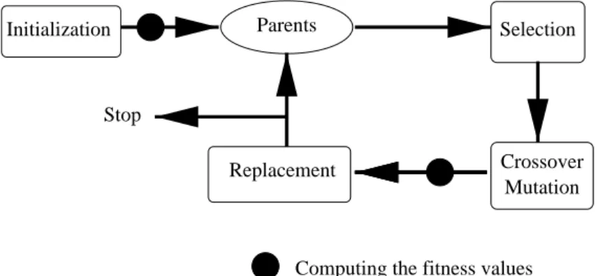
While most differ slightly in their actual implementations, all these evolutionary tech-niques use the same metaphor of mapping problem solving onto a model of evolution, where a candidate solution is represented by an individual and the solution quality is determined by a fitness function. The evolutionary process consists in evolving a vector (or population) of individuals, under stochastic modification and selection operators (see figure 1).
In contrast to many papers in the literature of Evolutionary Algorithms, we don’t fol-low the above described historical classification of algorithms. Rather, we review conver-gence results classified according to the model (e.g. Markov, schema, allele distributions),
Parents
Replacement
Selection
Crossover Mutation Initialization
Computing the fitness values Stop
Figure 1: A general description of Evolutionary Algorithms. – Initialization consists in selecting, usually at random and uniformly, a population of N individuals from the search space. – Selection consists in choosing a number (in the range [1, N]) of high fitness members that undergo Mutation and/or Crossover. – Mutation is an elementary modification operator. –Crossover combines the properties of two parents to produce an offspring. – In thereplacement step, a new population is selected among the current and modified individuals, such that the fittest individuals are more likely to survive.
space (finite, infinite) and operators (mutation, crossover). Then, we detail an alterna-tive Markov model GAs valid for finite or infinite search spaces, static or dynamic fitness environment, homogeneous or inhomogeneous operators. An overview of our approach is presented later on in this introduction.
1.1 Summary of the paper
We first review the modeling of homogeneous GAs in the binary spaceE ={0,1}`, where an individual is a sequence of binary bits (calledalleles). We describe approaches studying the evolution of population schemata ; population mean and variance in fitness ; population alleles marginal distribution.
We then point out the limitations of these approaches: the first approaches applies to infinite populations, the second applies to particular fitness functions, the third only models a particular type of GAs – basicly selection and crossover algorithms with no mutation.
We also review strong convergence results, about the complexity of the time to ab-sorption, that have been obtained for simplified and rudimentary GAs (selection only or mutation only).
The main general theoretical results in the field of evolutionary function optimization have been obtained using Markov chain analyses in finite spaces. These results prove the asymptotical absorption into optimal states w.r.t. time for the homogeneous GA ; and prove a finite time visits to the optimal set for the inhomogeneous GA. In this Markov framework, the state space is the set of all populations.
An alternative Markov approach considers the state space of all probability distribu-tions of the populadistribu-tions, rather than the space of populadistribu-tions. It proves the existence of
fix points for population distributions, for an infinite population size. In this framework, a distribution is a vector of length 2`, describing the proportion of each point ofE ={0,1}`
in the population.
In this paper we propose an alternative Markov approach on the space of population distributions. But, in contrast to the latter approach we consider the empirical measures (2) associated to the population (1), resulting in distributions having a small variable support, which length is equal to the population size.
A first advantage of this approach is that it also applies to infinite and continuous spaces. A second advantage is that it allows to build a bridge between the fields of genetic algorithms and that of interacting particle systems.
An important part of this paper is then devoted to applying some recent convergence results from the IPS literature to the simple mutation-only genetic algorithm. Note that the term convergence here is twofold. We (briefly) consider the long time behavior of GAs, and (widely) investigate the convergence quality and rate of the genetic algorithm, seen as a measure valued process, when the population size tends to infinity.
For example, when the population size tends to infinity, in some sense to be defined, the difference between the finite population empirical measure at timet and the measure it would have if the population size were infinite, goes to zero in ILp-mean. Analogous results also apply to the path space, involving a sequence of measures taken from time 0 to n, and provide large deviation bounds.
On the other hand, when the time parameter goes to infinity, we show that under some conditions, the distribution of GA (infinite) population at timenconverges exponentially fast to a unique fix point.
Last but not least, we generalize the IPS approach so as to cope with different variants of genetic algorithms.
For example, we consider mutations where the transition probabilities depend on the whole current population (and not only the point to be mutated). Such transition kernels naturally include special crossover mechanisms. We also investigate the convergence of GAs with commonly used crossover operators.
We end the paper by proposing a new dynamical system, corresponding to GAs with an original generational scheme: selection-or-mutation transitions rather than the common selection-and-mutation ones.
1.2 The IPS approach: preliminaries
In the following we outline the IPS approach, before presenting the related sections’ con-tents.
Genetic algorithms can be defined as a system of particles (or individuals) evolving ran-domly in a given measurable space (E,E) and undergoing adaptation in an environment, not necessarily time homogeneous, represented by a collection of fitness functions.
In discrete time settings these stochastic algorithms can be modeled as a Markov chain
ξn= ξn1, . . . , ξ N n
taking values in the product state spaceEN whereN ≥1 denotes the number of particles. Although it is not really essential the initial particle system ξ0 usually consists in N
independent particles with common law η0 ∈ P(E), where P(E) denotes the set of all
probability measures onE endowed with the weak topology.
Rather than studying the dynamic and limiting process of the so defined Markov chain (1), we propose to study the flow of the empirical measures associated with the systems of particlesξn
m(ξn)
def. = 1
N
N
X
i=1
δξi
n (2)
whereδa stands for the Dirac measure at a∈E.
The transition from the populationξn−1 at time (n−1) to the next populationξnonly depends on the empirical measurem(ξn−1). More precisely, given the configuration ξn−1
at time (n−1) the next generation ξn consists of N (conditionally) independent random variables with common law
Φn(m(ξn−1))
where Φn : P(E) → P(E), n ≥ 1, is a given collection of sufficiently regular functions, that are dictated by the GA operators and parameters (see section 7.1).
This quite general interacting particle system model has been introduced in [10, 11]. Its asymptotic behavior as N → ∞ is now well understood. In some sense to be defined the empirical measures
ηnN def= m(ξn), n≥0,
converge as the number of particles N → ∞ to a deterministic flow of distributions
ηn∈ P(E), n≥0, solution of the measure valued dynamical system
ηn= Φn(ηn−1), n≥1, (3)
In measure valued processes literature the system (3) is usually called the limiting process. Such measure valued dynamical systems have arisen in such diverse scientific disciplines as physics, biology, evolutionary computing, nonlinear filtering and elsewhere. In GA settings this measure valued dynamical system is sometimes referred as the infinite population model and it is used to predict the behavior of the finite population model. In advanced signal processing and particularly in filtering literature (3) represents the evolution in time of the conditional distributions of a signal given the observation record. Incidently theN-IPS approximating scheme of the nonlinear filtering equation is defined in terms of a time inhomogeneous and simple GA.
The continuous time version of this model is described in [7, 8] revealing a very striking analogy between GA, the robust and path-wise nonlinear filter, Feynman-Kac formulae and spatially homogeneous Boltzmann equation.
The objective of this paper is not to develop the details of all these connections between these research fields, the interested reader is referred to the monograph [7] and to [8]. Our
aim is to introduce the reader to IPS approximations of nonlinear measure valued processes of the form (3) and to present the mathematical theory that it is useful in studying the asymptotic behavior of GAs.
1.3 Organization of the paper
This paper is organized as follows.
Section 2 summarizes a number of approaches to GA modeling, so far encountered during the last decade, excluding the Markov models that are described in a separate section. These approaches does not lead necessarily to strong convergence results, but give insights into some aspects of GA dynamics under some approximations or in particular fitness cases.
Section 3 reviews results obtained on simplified and rudimentary processes, such as selection only or mutation only algorithms. These simplifications have the advantage of making theoretical analysis very amenable and allow one to compare complexity of time to convergence with different selection or mutation schemes. On the other hand, results obtained with such simplifications cannot be generalized to more complex and realistic (working) GA instances.
Section 4 presents different exact Markov models leading to the proof of the convergence of different classes of Genetic Algorithms towards the optima of the fitness function. While these results put almost no restrictions on the fitness function, they cannot give the order or complexity of convergence time.
Having introduced different models for Genetic Algorithms, related results and lim-itations, we introduce the IPS model for infinite populations, which can be seen as a generalization of the infinite population model of Vose [96], to the case of infinite search spaces. We then show how theN-IPS approximating model can be used to studyN -sized-population GAs.
A first advantage of the IPS model is that it allows us to model a wide variety of Genetic Algorithms, as shown in section 7. A second advantage is the existence of a number of recent theorems from probability literature that guarantee the convergence of the finite population dynamic of GAs (N-IPS approximating model) towards the infinite population dynamic (IPS model), for large populations uniformly with respect to time (these results are summarized in section 6 for an abstract and general IPS model). Finally, the Feynman-Kac interpretation allows us to derive the exact analytical distribution of GA population members.
In section 6 we describe precisely the IPS approximating model and we review recent results on the convergence of such IPS methods when the number of particles (or popula-tion size) goes to infinity, including weak convergence theorems, ILp-mean error estimates, exponential rates and large deviation principles.
Most of the limit theorems presented in this preliminary section 6 result from collab-orations of one of the authors with Alice Guionnet, Michel Ledoux and Laurent Miclo. Only a selection of existing results is presented. More information and detailed proofs can be founded in the set of referenced papers [1, 2, 3, 4, 6, 7, 10, 11].
All these developments offer the appropriate theoretical background to analyze the asymptotic behavior of GA. They also permit us to construct new genetic-type methods. In section 7 we present several generic GAs which fit into our framework including the simple GA with classical mutation and proportionate selection, but also GAs with interact-ing mutation, cross-over transitions and GAs with randomly ordered selection/mutation. We will also give a detailed illustration of how the convergence results presented in sec-tion 6 may be applied to study the asymptotic behavior of such GAs.
It turns out that many GAs including cross-over transitions fit into the simple GA framework. For these reasons, and because of the importance of the simple GA in prac-tice, section 7.1 is built around this theme. We complement the limit theorems of section 6 and we present several additional asymptotic theorems including a Central Limit Theo-rem, a limit theorem on the long time behavior of the limiting system as well as a uniform convergence theorem for theN-IPS approximating model with respect to the time param-eter.
We hope this paper will be useful to our colleagues working on GAs and evolutionary computing.
2
Different approaches to GA modeling
This section briefly presents a number of tentative approaches to GA modeling, excluding the Markov models that are described in the next section. We also present some alter-native algorithms that arose from some of these modeling approaches. Such alteralter-native algorithms also intend to achieve a stochastic optimization task, but at a reduced cost compared to the standard Evolutionary Algorithms described in figure 1. Most of these approaches consider search spaces of binary stringsE ={0,1}`, where a string is viewed as a vector of`binary alleles.
Section 2.1 recalls and comments on the schema theory, modeling the evolution of schemata. Section 2.2 presents and comments on an approach borrowed from physics, approximating the evolution of population fitness distributions by some of their moments. Section 2.3 focuses on the evolution of allelic marginal distributions. This latter point of view has been given much attention in the last 5 years, and led to a number of alternative algorithms, that are not guaranteed to find the global optimum, but which might converge quicker than GAs.
2.1 The Evolution of Schemata
Initial investigations about binary Genetic Algorithms (GAs) concentrated on a macro-scopic view of the algorithms, based on the evolution of schemata (rather than strings or proportions of strings, as in the Markov framework). A first version of the schema theorem was proved in [55] then an extension in [47].
The framework is the following. Consider the binary spaceE ={0,1}`, a proportionate selection, a 1-point crossover and a 1/` mutation.
A schema is defined as a subspace H of E where a number, denoted o(H), of string positions have fixed values. For example, the schema (1∗11) ={1011,1111} has 3 fixed
values.
Theorem 2.1 ([55, 47]) Let N(H, n) be the number of representatives of H in the pop-ulation at time step n, then, neglecting the possible reconstruction of new representatives of H by mutation or crossover,
IE[N(H,n+1)]≥ N(H,n)
¯f(H,n) ¯f(ξ
n)
1−pmo(H)−pc l(H)
`−1)
, (4)
wheref¯(H, n)denotes the average fitness of representatives of Hpresent in the population
ξn, and l(H) denotes the distance (number of positions) between the first and last fixed
positions of H ( l(H) = 4 in the previous example), pm and pc denote the mutation and
crossover probabilities.
Under infinite population approximation, the expectation of the number of schema repre-sentatives can be replaced by its actual value in (4), one obviously conclude that schemata with above average fitness ( ¯f(H, n)>f¯(ξn)) tend to colonize the population.
The usefulness of the Schema Theory has been seriously questioned [52, 93, 71, 63, 19, 97, 36, 22]. One of the main limitations of the Schema theory is that it is only valid for one generation prediction and cannot be iterated more than once (as it maps a schemata into the next expected one only), hence cannot be used for studying the long term behavior.
Recent work [17, 84, 85, 96] prove a new relation for the evolution of schemata, taking into account the effect of schema reconstruction by crossover and mutation (and so ac-counting for possible low fitted schemata that yield high fitted offspring), but still falling under the limitation of relating the expectation of N(H, n+ 1) to N(H, n) as explained above.
Note finally that, at its current stage, the schema theory still doesn’t lead to any strong theoretical result about convergence, or complexity of the algorithm itself.
2.2 Cumulants of Population Fitnesses
In the statistical mechanics formulation [29, 99, 72], a population is described in terms of a few macroscopic quantities: thecumulantsof the populationmagnetization distribution. Thecumulantsdenote the meank1, variancek2 (and eventually moments of higher order)
of the populationmagnetization distribution. The magnetization of a string is defined as
M(x) = `
X
i=1
xi where xi ={0,1}. (5)
For most problems the fitness distribution is not related to the magnetization distribu-tion. However for simple examples such as one-max, magnetization equals fitness. Thus many papers study the evolution of expected population cumulants, providing recurrence relations between the expected cumulants when mutation (resp. selection, or crossover) is applied to population members, in a generational scheme (see [14] for a detailed review of the approach and simplification hypothesis).
Under the usual assumption that only the – 2,3 or n – first order cumulants are non null, [99, 100] prove the following relation whenN individuals are selected following Boltzmann selection with small strength β, the change in cumulants – when terms of higher powers ofβ are truncated – follows from [99, 100].
< κ1 >S ' < κ1 >+< κ2 > β,
< κ2 >S ' < κ2 >−
< κ2 >
N +< κ3 >β.
where the subscriptS denotes that this is the effect of selection.
When mutation is applied to all population members with bit-wise-flipping probability
c/`.
< κ1>M = (1−2c) < κ1 >, (6)
< κ2>M = (1−2c)2 < κ2 >+`(1−(1−2c)2), (7)
where the subscriptM denotes that this is the effect of mutation, and< . > denotes the expected cumulant value over anensemble(infinite set) of populations evolving in parallel. Combining these expressions, to find the expected cumulants after selection, mutation (and eventually crossover (15)) is straight-forward for the onemax function, but can be unwieldy for more complex functions, in such cases the formulae are simulated numerically. This approximated model has been extended to other generational and selection schemes and also demonstrated to be quite close to the actual behavior of GAs averaged over many runs [75, 14].
This approach has also been applied to study the dynamics of GAs on functions dif-ferent from one-max, but in most cases, the fitness is a function of the magnetization (or Hamming distance to all-ones optimum) [82, 76].
At the cost of some approximations, this statistical mechanics model allows us to gain significant insights into the population dynamics on a number of fitness functions. These results would be difficult to obtain at this stage using exact models of GAs such as Markov chains. Indeed, apart from particular cases [57, 43], Markov chain studies of GA exact dynamic consider populations of size one and no crossover, on simple functions (see section 5).
2.3 Allelic Marginal Distributions
This modeling approach is in some ways similar to the one we are presenting in the paper – namely, the interacting particle systems model (IPS). However, the goals are different. The IPS model is used to study the convergence of the dynamic of finite population GAs towards that of the infinite population GAs, whereas the following model is used to construct alternative stochastic algorithms, with a smaller time to convergence than GAs. The basic idea is to transform the initial search problem over E into a search problem over probability distributions onE. The target probability distributions are then mixtures of Dirac distributions charging optimal solutions of the initial search problem overE.
The model we describe in this section was first proposed in practical numerical simu-lations [23]: selected population members are no longer mutated and mated, but used to update the allelic marginal distributionspi, as follows.
pi(xi, t+ 1) =pi(xi, t) +λ psi(xi, t)−pi(xi, t)
, (8)
wherepsi(xi, t) are the marginal frequencies of allelexiin the selected population members. The new population is then constructed by drawing N stringsx = (x1. . . x`), according to the probability profile
p(x, t+ 1) = `
Y
i=1
pi(xi, t+ 1).
The convergence speed of this algorithm (8) critically depends onλ. For λ= 0 we obtain a random search, for λ= 1 we obtain the so called UMDA algorithm [65]. M¨uhlenbein formalizes the UMDA algorithm, in the infinite population framework, with proportionate selection (10) and complete crossover, but no mutation. He shows that this algorithm consists in performing a gradient search with the potential W(t) = Pxp(x, t)f(x) [65], (that is, the average fitness),
p(xi, t+ 1) =p(xi, t) +p(xi, t)(1−p(xi, t))
∂W /∂p(xi)
W(t) (9)
wherep(xi, t) denotes the probability that xi = 1 at time t. However, this gradient is not easy to implement directly asW(t) requires the knowledge of 2` parameters.
In order to search directly in the space of distributions, another approach consists in reducing the complexity of the distributions space. This can be achieved by restricting the search to a family of parametrized distributions, allowing one to simply search in the parameter space. This is a typical approach in the learning field.
This approach is illustrated in [24] where the vector x = (x1, . . . , x`) of E is replaced with a vector of`random variables with a vector of respective parametrized density profiles
p(x, θ) = (p1(x1, θ1), . . . p`(x`, θ`)),
where pi(. , θi) defines the distribution of allele xi over {0,1}, parametrized by θi. For example, numerical simulations of [24] assumepi(. , θi) as independent Bernoulli laws (resp. gaussian) with average θi (resp. average and variance given by θi components).
The discrete optimization problem in E is then transformed into a continuous mini-mization problem of the Kullback-Leibler (KL) divergence [101] between pand the Gibbs distributionp∗T, which charges the high fitness states ofE for low temperatures T. It can be shown that this minimization can be achieved with a gradient in the space of the free energy of the system F(θ) [24]. Yet as for W(t) above (9), computing the free energy requires the knowledge of 2` parameters.
In order to make this gradient minimization computationally amenable, Berny [24] proposes approximate (and stochastic) update (gradient following) rules for θ, allowing him to successfully minimize the free energy on a number of fitness functions, and for
different temperatures. However, due to the approximations, the asymptotical convergence to the global optima is not guaranteed on a given fitness landscape.
Note finally that more robust algorithms could be obtained, if dependent random variables were considered for allelic distributions, as pointed out in [24] and [65].
3
Convergence of simplified algorithms
In any evolutionary algorithm, the strong interactions between selection and evolution operators (crossover, mutation, . . . ) make it difficult to efficiently compare the effects of different operators without taking into account the characteristics of the selection (i.e. the fitness function).
A standard method for avoiding such a bias, is to start by considering the effects of each operator alone: Selection without evolution operators (see the studies of takeover time [49, 34]), or innovation time of crossover or mutation in the absence of selection [88, 48], or the evolution of random walks directed by some mutation [45] or crossover [31] operators.
In the following, for the sake of clarity, the reported results do not always cover the whole set of extensions and generalizations that could have been achieved in the papers, but mainly focus on the techniques used to find the results (for example we might omit to mention extensions of formulae to r-ary alphabets).
3.1 Selection only algorithms
Consider a finite population of N members ξ ∈ EN and suppose some members of the population ξ are selected possibly more than once in order to form a new population of size N. This defines a rudimentary dynamical process and we are usually interested in calculating the time required to reach a population withN copies of a same member.
ξn−1= ξn1−1, . . . , ξ
N n−1
Selection
−−−−−−−−−−−−→ξn= ξn1, . . . , ξ N n
This is a widely studied in both the literatures of genetic algorithms and populations genetics. However, the approaches and selections involved differ significantly.
In the context of genetic algorithms, we are interested in problem solving, hence se-lection directly depends on the fitness of population members: high fitted members are more likely to be selected than low fitted ones. Typically, with a proportionate selection the probability to select thei-th individual of ξn−1 is given by
f ξni−1
PN
j=1f
ξjn−1
(10)
At each iteration,N individuals are selected following (10), that build up the population
ξn (see Table 3.1 for alternative typical iterations). Other typical selections are Ranking selection (same as (10) replacing fitness values by their rank in the population), and tournament selection (p members are chosen uniformly, and the fittest is selected).
In the genetic algorithms literature, early studies use Markov chains to numerically calculate the expected absorption time. This is achieved by calculating the visitation matrix V = (I −Q)−1, after partitioning the states of the absorbing Markov chain (ξn) associated with the selection algorithm,
P =
Q R 0 I
.
Summing over the set of transient states T S, Pj∈T SVij, yields the expected absorption time for a process starting at statei. This method was first applied in the spaceE={0,1}
with proportionate selection [51].
The impact of selection with sharing 1 has been investigated using the same method and space E = {0,1} [56], demonstrating that the expected absorption time is signifi-cantly larger with sharing (simulated for various small population sizes and various ratios
f(1)/f(0)).
An original issue is also addressed in the same paper [56]. The author studies the “quasi-equilibrium state” of the chain before absorption (as absorption time is very large with sharing). This corresponds to finding the quasi-stationary distribution of matrix Q (as defined in [35] for near-ergodic absorbing Markov chains).
Also in the Markov framework, [60] considers the general case ofE={0,1}`and shows, under some simplifications, that Boltzmann tournament selectionhave the same effect of maintaining the diversity in the populations resulting in a larger expected absorption time. Still from the GA literature, a different approach to selection algorithms approximates the recurrence between the proportionpnof the optimumx∗ at each generation (valid for infinite populations),
pn'
f(x∗)pn−1
¯
f(ξn−1)
In the space E ={0,1} [18] solves this recurrence, showing that starting from a random uniform population, expected time to have a proportion 1−1/N of the optimum (say individual 1) is
ln(N −1)
ln(f(1)/f(0)) (11)
Again under the infinite population approximation, different types of selections are studied and compared in the continuous space E = [0,1] [49]. Results are summarized below, showing that starting from a population containing one optimum, the expected time to reach a proportion 1−1/N of the optimum, have a complexity ranging from O(lnN) to
O(NlnN).
1
Sharing [50] tends to spread the population out over multiple peaks in proportion to the height of the peaks. For example, if there arem individualsykin a Hamming radius ofσfrom local optimumx, their
Generational Selection Takeover time
Proportionate 1
c(NlnN−1), forf(x) =x
c
1
c(NlnN), forf(x) = exp (c x)
Linear ranking 1
ln 2(lnN+ ln lnN), forc= 2 byr(f(x)) =c−2(c−1)x, 2
c−1log(N −1), for 1< c <2
p-Tournament 1
lnp(lnN+ ln lnN)
In the population genetics literature, selection is usually uniform on the population. The progressive loss of diversity in the population is then called genetic drift. Analysis of genetic drift is often performed by calculating the Markov chain transition matrices in order to analytically approximate the time to absorption [62, 58].
An alternative approach to genetic drift consider the rate of decrease in population fit-ness variance under uniform selection [68, 67, 72], and lead to an exact analytical approach in many cases (see [74] for a quick overview). The ratio between population variances after one generation is given below (the first is exact and the others are approximations accurate up to terms of order 1/N).
Iteration loop ratio of fitness variance of successive populations Generational
(chooseN members independently 1−1/N and uniformly inξn−1 to formξn)
Generational gap G
(chooseGN members uniformly, that 1−(2−G)/N, for 0≤G≤1 replaceGN members uniformly chosen)
CHC type
(duplicate each member ofξn−1, then 1−1/(2N)
deleteN members uniformly chosen)
These studies are half way between population genetics (as the selection is fitness-independent) and genetic algorithms as different typical iterations are compared for the same selection. These results show that genetic drift for a CHC iteration is slower (at half the rate) than for the traditional generational iteration, which in turn is slower than generational gap and steady-state (obtained forG= 1/N) iterations.
Genetic drift is usually seen as the responsible for the often observed problem of prema-ture convergence. That’s why such results obtained for selection algorithms can be helpful in guiding GA practicers in the choice of selection schemes and iteration loop according to the problem at hand.
3.2 Random walks on operator-neighborhood graph
Consider a finite population of N members, ξ ∈ EN, and suppose each member of the population undergoes a mutation, transforming ξnk−1 intoξnk, fork = 1, . . . , N.
ξn−1 = ξn1−1, . . . , ξ
N n−1
Mutation
−−−−−−−−−−−−→ξn= ξn1, . . . , ξ N n
(12) In the binary space E = {0,1}`, two typical mutations are compared [45]. For large `
values, it is shown that the hitting time of solution obeys an exponential distribution with respective means
2`
N(1−e−c), for the c/`mutation (flips each bit with probability c/`), 2`
N, for the 1-bit mutation (flips exactly 1 bit uniformly chosen).
In other words, this result shows that the widely used (positive) c/`mutation is clearly outperformed by the simple 1-bit mutation (in terms of the probability that the optimum has already been hit) at each time step.
Again in the binary space E = {0,1}`, but for large population sizes and only for the c/` mutation, the whole dynamic of the algorithm can be described in terms of the distribution of the population magnetization (average number of ones in population mem-bers, as detailed in section 2.2). Equations (6) and (7) provide an approximate recurrence relation between the expected average and variance of the population magnetization at successive generations.
The case of populations evolving under crossover has also been addressed. Consider
N random couples selected uniformly and independently in ξn−1. Each couple is mated,
resulting in N offspring that build up the next population.
ξn−1 = ξn1−1, . . . , ξ
N n−1
Crossover
−−−−−−−−−−−−→ξn= ξn1, . . . , ξ N n
In the context of infinite populations, general results can be found in [46, 30] which prove that all complete2 crossover schemes lead to the same limit distribution, given by Robbins proportions of individuals in the limiting population.
π(x) = `
Y
i=1
p(xi), (13)
where p(xi) is the constant marginal distribution of the allele at position i. Note that these marginal distributions do not change when crossover is applied.
Recently, [31] proved that finite populations of r-ary strings under crossover converge in average to the populations with Robbins proportions. This result assumes that the application of crossover can produce any combination of parents alleles.
2
The case of finite populations has been widely investigated [99, 100] using statistical mechanics techniques in the binary framework, introduced in section 2.2. Averaging over all the ways of performing bit-wise crossover, the expected mean and variance of population magnetization is given by the recurrence relations
µc = µ, (14)
σc2 = (a2+ (1−a)2)σ2+ 2a(1−a)`(1−q)
4 , (15)
where ais the probability we choose an offspring allele from parent x and (1−a) is the probability that we choose an offspring allele from parenty, and
q = 1
N(N−1)
X
x6=y 1
`
`
X
i=1
(2xi−1)(2yi−1)
!
,
is the pair-wise correlation between population members. Hence crossover increases the population magnetization variance towards `(1−q)/4 at a rate which is maximized for
a= 0.5, and does not change the mean magnetization of the population.
As a conclusion, these results obtained for rudimentary versions of algorithms certainly allow one to obtain theoretical bounds on convergence for different operators and selec-tions, but these results cannot be generalized to general GA instances using mutation, crossover and selection, nor do they allow us to prove the convergence of GAs as function optimizers, in a general function context.
4
Three Markov approaches to GA convergence
The main theoretical results in the field of evolutionary binary function optimization have been obtained using Markov chain analyses. The two first approaches are Markov chains in the space of the GA populations; the third approach is a Markov chain in the space of the distributions of population members inE.
4.1 Homogeneous Genetic Algorithms in finite search spaces
Historically, it has been quite natural to model GAs as Markov chains where the “state of the GA” at time step nis given by the current population (viewed asN individuals)
ξn= ξn1, . . . , ξ N n
. (16)
The state space is then the product space EN, where N ≥ 0 denotes the number of individuals in a population, and the initial population ξ0 usually consists of N random
individuals uniformly chosen inE.
ξn−1
Selection
−−−−−−−−−→ξbn−1
Mutation
We shall give the transition probabilities in the case of a generational GA, with pro-portionate selection, fitness function f, and mutation kernelK fromE into itself.
At each iteration, N individuals are selected following (10), that build up the popu-lation ξbn−1. Each member of the selected population ξbn−1 undergoes a mutation. The
transition can be summarized, for eachn≥0, as follows
IP (ξn+1=x|ξn=y) = N
Y
p=1
N
X
i=1
f(yi)
PN
j=1 f(yj)
K yi, xp, (17)
whereK yi, xpgives the probability that individualyi ∈E is mutated into xp.
The mutation operator is at the core of all convergence results obtained so far in the GA literature, as irreducible mutation is often responsible for the reachability of all states in a finite time. More precisely, we have the following theorem by well known Markov Chain results, proving the convergence with probability one towards optimal states. Theorem 4.1 ([53]) If the sequence of populations-best-fitness is monotone (increasing if maximizing) with respect to time; and if any point ofE is reachable by means of mutation and recombination in a finite number of steps, then
IP(limn→∞x∗ ∈ξn) = 1. (18) Note that the monotonicity can easily be achieved by considering an elitist selection or an adequate iteration loop guaranteeing the survival of the best individual at each generation. For example, with a steady-state iteration, at each iteration an individual (chosen with any selection) undergoes mutation and crossover, then replaces the individual with the worst fitness in the population.
Analogous general theorems exist for large classes of evolutionary algorithms in infinite real-valued search spaces, as Evolutionary Programming and Evolution Strategies. In fact, these algorithms can be seen as particular cases of the global random search algorithm which convergences with probability one towards optimal states [98]. The reader is referred to [22] (pages 48–51) for a discussion of the connection between these continuous space algorithms and the uniform and global random search algorithms.
This Markov chain model has been adopted in many papers, where some convergence proofs are provided for specific GA instances mainly in the space E={0,1}` and for the widely used positive 1/` mutation.
For example, Rudolph’s convergence results [78, 77, 80] directly rely on the positivity3 of the mutation operator, while their extension by Agapie [16] relaxes the strong hypothesis of positive mutations to the irreducible4 and diagonal positive transition mutation matrix. Both these authors emphasize that the monotonicity condition can be fulfilled virtually by maintaining and updating the best so far individual in the population without it taking place in the evolution process. In other words, the sequence of best fitnesses found so far by GA populations converges almost surely to the optimal value of the fitness function,
3there exists a mutation that links any two points of the space with non-zero probability 4
when an ergodic GA is used. On the other hand, Agapie [16] shows that the monotonicity condition is necessary for the convergence with probability one (as in equation 18) of the homogeneous GA with proportionate selection and irreducible mutation.
Note finally that nearly all convergence results for the homogeneous GA prove that the best so far individual of the population enters the optimal set with probability one (18). On the other hand, the inhomogeneous parameters of Cerf’s GA (next section), allows him to prove first, the absorption of all population members towards the optimal set almost surely, and second, finite time visits to the optimal set.
4.2 Inhomogeneous Genetic Algorithms in finite search spaces
Also in the Markov framework, other results have been obtained with techniques, similar to those used to prove the convergence of simulated annealing [89, 90] : a genetic algorithms is seen as a stochastic perturbation (mutation, crossover) of a deterministic dynamical system (selection only). The rate of these perturbations goes to zero with time going to infinity.
Some preliminary results obtained by Davis and al. [37, 38], consider populations as a vector describing the number of occurrences of each individual in the population, (the same as the population vector described in next section for homogeneous GAs (21)). The authors prove the convergence of an inhomogeneous GA towards populations with identical individuals. More recently, Suzuki [87] builds on Davis model, and proves the asymptotical convergence to optimal states.
These results are largely extended by Cerf [32, 33] using the same Markov model as last section, where a population is defined as a vector ofN individuals (16).
Using the Friedlin-Wentzell theory of stochastic perturbation of dynamical systems [61], Cerf obtains a lower bound for the population size allowing him to prove finite time convergence results for the inhomogeneous Genetic Algorithm detailed below. His results are primarily based on mutation (but he shows that an acceleration of convergence might be brought by crossover, in the sense that the lower bound on population size is smaller when crossover is used).
Cerf’s results emphasize a decreasing mutation rate, tightly coupled to an increasing selection pressure, to reach finite time convergence (absorption of all the members of the population in the set of optimal points). More precisely, this result holds if the probability of mutatingx intoy is given by the kernel
αk(x, y) =
α(x, y)k−a, ifx6=y
1− X
z∈E, z6=x
αk(x, z) ifx=y
and the probability of selecting an individualyi in a populationξ is
βk(yi, ξ) =
ec f(yi)ln(k)
Pm
j=1ec f(xj)ln(k)
whereα is an irreducible mutation kernel onE, and k is a parameter that tends to infinity such that λ, the radius of convergence of the series S = Pt∈INk(t)−θ is in the range
θ1< λ < θ2 (θ2 andθ2 are dictated by the fitness function).
Finally, Cerf provides a functionN∗ such thatN > N∗(α, f, a, c) ensures the following results.
∀x∈EN, limn→∞IP([ξn]∈f∗|ξ0=x) = 1, (19)
∀x∈EN, IP(∃N, ∀n≥N , [ξTn]∈f∗|ξ0=x) = 1, (20)
whereTn is the time of then-th visit to the set of populations with equi-fitness values, f∗ being the class of optimal populations. Equation (19) ensures the absorption in the optimal states with probability one, while (20) ensures finite time recurrent visits to populations with optimal states only.
An alternative inhomogeneous algorithm has been proposed [42], where the firstK(n) points of the population vector undergo a random mutation, and the others are replaced by the optimal point at each generation. The proof of convergence relies on the Perron-Frobenius theorem and shows that ifK follows a binomial law with a parameter going to zero at the rate p=n−1/D (whereD denotes the diameter of the mutation graph), and if the population size is large enough (a sufficient condition isN > D), then
∀x∈EN lim
n→∞IP([ξn]∈f ∗
/ξ0 =x) = 1.
Note that these inhomogeneous GAs are not used in practice as the rate of decay of the perturbations is too slow to be implemented, and the required population size is too big. However, one can expect these results to be improved under some assumptions on the fitness function.
4.3 Dynamical Systems model for Homogeneous GAs
When the search spaceE is finite, and the fitness function is constant (homogeneous with respect to time), then there is a model describing the simple genetic algorithm (selection, mutation, and cross-over) called thedynamical systems model. The analysis is best devel-oped for GAs with proportional selection, although others (rank-based, tournament) can be described within the framework. There has also been some work done on analysing fitness functions which are periodic with respect to time (see, for example, [107, 103, 106]) The existing theory is largely due to Michael Vose, and is described in detail in [96] (and see [104] for a simple introduction). The idea is to represent populations as vectors
pn= (p1n, . . . , pdn), n≥0, (21) taking values in the unitd-simplex ∆d ⊂IRd with
d= Card(E) and ∆d =
(
x∈IRd ; xi ≥0 d
X
i=1
xi = 1
)
wherepkndenotes the proportion of thek-th individual of the search space in the population at time step n. We are then interested in the trajectory of the population through the simplex, which defines a Markov chain (pn), n ≥ 0. Notice that a vector p ∈ ∆d has a dual interpretation. It represents an actual (finite) population, but it can be viewed as a sampling distribution for choosing a new population. In the infinite population framework, both these points of view can be confused.
Given a population pn at time step n, we define an operator G : ∆d → ∆d such that
G(pn) is the sampling distribution for the population at time step n+ 1, so that in the inifinite population framework we have,
pn+1 =G(pn) (22)
and in the finite population framework we have, IE[pn+1] =G(pn).
This operator G can be broken down into three parts, one for each of selection (F), mutation (U) and cross-over (C), with
G=C ◦ U ◦ F
For certain typical definitions of these operators, it turns out that mutation and cross-over commute. The combined effect of these operators is called themixing operator, denoted
M.
Given a populationpnat time stepn,G(pn) defines the sampling distribution for choos-ing a new population. Such a population may be chosen by samplchoos-ing the k-th individual with probability G(pn)k. This is a multipnomial distribution, hence the probability that this results in a specified populationq, is
IP(pn+1=q|pn=p) =N! s−1 Y
j=0
(G(p)j) N qj
(N qj)!
(23)
whereN is the population size.
In addition to representing the sampling probabilities for the next population, G(pn) is the expected next population. As N → ∞, the variance of the sampling shrinks to zero. In effect, the trajectory of the markov chain tends (in some sense to be defined in Theorems 6.3 and 7.6 using the IPS model of GAs) to the deterministic sequence
p0,G(p0),G2(p0),G3(p0), . . .. For this reason, this model (22) is sometimes referred to as
theinfinite population model.
It should be noted, however, that properties of this (infinite population) sequence do give us information about finite populations. In particular, regions in which kG(p)−pk
are small enough5 will, by a continuity argument, be regions in which a finite population will spend some period of time. Such regions (for example, those around fixed points of
G) are referred to as metastable states [102, 108].
5Whether this is possible – to closely approach any real numbers by fractions ofN – is out of the topic
An other recent direction of research has been proposed by [31]. He investigates the link between an abstract property π of a finite population and that of an infinite population. He proves that a sufficient condition for having π(IE[pn+2]) = π(G2(pn)) is that π be a
linear operator on the finite populations vectors and that for all finite populations pn,
π(G(pn)) =απ(pn+1).
Each of the three GA operators (selection, mutation and cross-over) are thought of in terms of their action on the simplex ∆d. Proportional selection is a scaled linear operator:
F(p) = Sp
kSpk1
whereS is a diagonal matrix with
Sk,k =f(k)
for each individual k. Mutation is a linear operator. It is given by a matrixU, in which
Ui,j is the probability that individual j mutates to become individual i. Then
U(p) =U p
Suppose we have a bilinear operator B : IRd ×IRd → IRd, so that B is linear in both parameters. Then a mapping Q: IRd→ IRd defined by
Q(x) =B(x, x)
is called a quadratic operator. Cross-over is given by just such an operator. It can be represented by a set ofdmatrices, C1, . . . , Cd, in which thei, j-th component ofCkis the probability that individualsiand j will cross-over to form k.
When the GA has no cross-over, its analysis is relatively straight-forward, as it is a (scaled) linear system. For example, a fixed-point of G satisfies
U Sp=λp
where λ is the mean fitness of p. Thus fixed-points are eigenvectors of the matrix U S. The Perron-Frobenius theorem ensures that there is eactly one such eigenvector in ∆d, corresponding to the largest eigenvalue. Other eigenvectors may be significant, for example by creating metastable regions, as described above, if they are near to the simplex.
When there is cross-over, the situation becomes harder to analyse. The fixed-point equations, for example, form a set of simultaneous quadratic equations. However, the situation can often be dramatically simplified. This happens when crossover and mutation are designed to respect structural symmetries that exist in the search space. This is the case, for example, when the search space comprises fixed-length binary strings, with the usual forms of cross-over and mutation [96]. However, the theory can be generalised to apply to any finite search space with a given group structure [105]. As an example of the kind of results that can be obtained, it is possible to diagonalise the cross-over matrices
C1, . . . , Cd by applying a Fourier transform, if and only if the underlying group structure is abelian.
It will become clear, as the paper progresses, that the dynamical systems model (22) is a special case of the IPS model (24). It corresponds exactly to the case whereE is finite, and fitness is homogeneous with respect to time. For this special case, there are a number of theorems which describe the behaviour of the simple GA. However, there are also a number of open questions. One of the most intriguing issues is the extent to which results which have been proved for finiteE can be generalised to infiniteE, and also the extent to which results which have been proved for infinite populations apply to finite populations. Recasting the dynamical systems model as an N-IPS model will help to establish both these questions. In particular, convergence properties of the finite population GA when
N tends to infinity, can be addressed directly using the N-IPS model, and these results are presented in Theorems 6.1 and 6.2 for a general IPS model, and in Theorem 7.2 and 7.6 for a Genetic-type IPS model.
5
GA behavior and Complexity results on particular fitness
functions
None of the results of last section make any particular assumption6 on the fitness function. But on the other hand, they do not give any indication about the complexity of the algorithm: the expectation of the number of generations required to reach the optimum remains unknown.
5.1 Finite spaces
In binary spaces E = {0,1}`, the first results about complexity give the expected first hitting time of the solution [20, 64, 21, 81] on the simple, well-studied, OneMax problem [15] (f(x) =P`i=1xi).
Recently, these results have been extended by Markov chain techniques, giving the variance of convergence time with different mutations [45]. Another well-studied problem is the long k-path (optimizable with a 1-bit-flip hill climber in exponential time w.r.t. string length) where expected convergence time [79, 39] and variance of convergence time have also been analytically derived [44] as a function of string length and population size. This study examines the simplified situation where the optimal population size is one. Furthermore, the GA withc/`mutation and proportionate or ranking selection takes a super-polynomial time to solve a sub-class of long k-path problems, although these functions present only one local optimum in the Hamming space. This latter paper also answers the challenging issue of existence ofcontrolled paths forc/`mutation GAs.
By definition, GAs are stochastic population-based algorithms. It makes little sense to exactly control the composition of the successive populations. Rather, we say that a GA follows acontrolled path when the best individual of the population visits a number of predefined points in the search space in a predefined order during the course of its run. This issue is addressed in [57]: A family of controlled-path functions is constructed, based on an arbitrary choice ofkeyswhich define a path in the search space. Experiments
6
show that the trajectory of elitist GAs with crossover and mutation, follow this path at each run.
5.2 Infinite spaces
In real-valued spaces E= [−b, b]`, an exhaustive set of results have been obtained for the corridor (f1(x) =c0+c1x1) and sphere (f2(x) =P`i=1(xi−x∗i)2) fitness functions, since the early days of Evolution Strategies (abbreviate ES) [73, 83]. In the case of the sphere model (f2), it is shown that for large `, log(ft/f0) ' t, where ft denotes the smallest fitness found at timet.
The most recent and powerful results provide bounds for the Euclidean distance to the solution in different situations. Beyer [25, 26, 27, 28] handles sophisticated variants of ES (i.e. based on Gaussian mutations with self-adaptive mutation parameters), while Rudolph [80, 81] studies the local convergence speed for a larger class of mutation operators.
6
The Interacting Particle System model of GAs
As discussed in the introduction, we can associate with the Markov chain modeling GAs on the space of populations (ξn)n≥) (1) with transitions (17), a measure valued process
(m(ξn))n≥0wherem(ξ) is the empirical measures associated with the populationξn, defin-ing a uniform distribution over the population members.
Alternatively, we can associate with any abstract measure valued process (24) an N -interacting particle approximating model, defining a finite population GA, as in (25). In this case, the mutation/selection transitions are dictated by the form of the limiting measure valued dynamical system (24). We illustrate this fact in the following section.
We first describe the Interacting Particle model, and limiting behavior with detailed convergence results. Then, we show how these results impact on standard GAs (section 7.1), GAs with crossover (section 7.3) and interacting (fitness dependent) mutations (sec-tion 7.2). We finally show how these developments permit us to construct and study new genetic algorithms (section 7.4).
6.1 Description of interacting particle processes
Consider a measure valued process of the form
ηn= Φn(ηn−1), n≥1, (24)
where {Φn ; n ≥ 1} is a given collection of continuous functions from P(E) into P(E). The N-IPS approximating model associated with this measure valued process is defined in terms of anEN-valued Markov chain
ξn= ξn1, . . . , ξ N n
, n≥0,
with transition probability kernels
P(ξn∈dy|ξn−1 =x) =
N
Y
p=1
wheredydef= dy1×· · ·×dyN is an infinitesimal neighborhood of the pointy= (y1, . . . , yN)∈
EN and x= (x1, . . . , xN)∈EN and where
∀x= (x1, . . . , xN)∈EN, m(x) = 1
N
N
X
i=1
δxi ∈ P(E), (26)
The initial system ξ0 = (ξ01, . . . , ξ
N
0 ) consists of N independent particles with common
lawη0.
This IPS algorithm can be described as follows:
• At the timen = 0 the particle system consists of N independent random particles
ξ01, . . . , ξ0N. with common lawη0.
• At the timen≥1 the empirical measurem(ξn−1) associated with the particle system
ξn−1 enters in the plant equation (3) so that the resulting measure Φn(m(ξn−1))
depends on the configuration of the system at the previous time n−1.
• Finally, the particle system at the time nconsists of N independent (conditionally to ξn−1) particlesξn1, . . . , ξnN with common law Φn(m(ξn−1)).
The above description enables us to consider the particle density profiles
ηnN =m(ξn) = 1
N
N
X
i=1
δξi
n, n≥0,
as a measure valued Markov process with transition probability kernel given by
IE F(ηNn)ηnN−1=
Z
EN
F 1
N
N
X
i=1
δxi
!
Φn ηNn−1
(dx1). . .Φn ηnN−1
(dxN),
for any F : P(E) → IR in the set Cb(P(E)) of all bounded continuous test functions on
P(E).
6.2 Asymptotic Behavior
This section is concerned with the asymptotic behavior of theN-IPS approximating model as the number of particles N tends to infinity.
It is divided into three parts. Section 6.2.1 covers weak law of large numbers results. In section 6.2.2 we propose an easily verifiable Lipschitz condition on the one step mappings
{Φn; n≥1} under which one can derive ILp-mean error estimates and useful exponential rates. Section 6.2.3 focuses on large deviations principles. These results complement and strengthen the distributional limit theorems presented in section 6.2.1.
The investigation of these asymptotic results require quite specific mathematical tools. To each of these approaches and techniques correspond an appropriate set of conditions on the one step mappings {Φn; n≥1}. We provide no examples in this section; this choice
is deliberate. Several detailed and precise examples of GAs satisfying these conditions will be given in the further development of section 7.
We also emphasize that when the state space E is finite most of these conditions are easy to interpret mainly because in this situation the set of all probability measuresP(E) coincide with the unit d-simplex ∆d ⊂IRd with
d= Card(E) and ∆d =
(
p∈IRd ; pi≥0 d
X
i=1
pi= 1
)
.
6.2.1 Weak Law of Large Numbers
The approximation of dynamical system (24) by the N-IPS approximating model (25) involving the empirical measuresηnN, is guaranteed by the following Theorem.
Theorem 6.1 ([11], p. 448.) If E is compact then we have that
∀F ∈ Cb(P(E)), ∀n≥0, lim
N→∞IE F(η
N n)
=F(ηn). (27)
More generally (27) holds when E is locally compact and the mappings Φn, n ≥ 1, are uniformly continuous.
We now give some comments on Theorem 6.1.
By Bb(E) we denote the space of all bounded Borel measurable functionsf :E →IR and byCb(E) we denote the sub-space of all bounded continuous functions. For anyf ∈ Bb(E) and µ∈ P(E) we write
µ(f) =
Z
E
f(x) µ(dx).
One consequence of (27) is that for anyF ∈ Cb(IRd),d≥1, andf1, . . . , fd ∈ Cb(E) and for any n≥0
lim
N→∞IE F(η
N
n(f1), . . . , ηNn(fd))
=F(ηn(f1), . . . , ηn(fd)).
Applying this result one can obtain the limit of the ILp-moments of the particle density profiles errors. More precisely for any n≥0 and p≥1 andf ∈ Cb(E) we have that
lim N→∞IE
ηNn(f)−ηn(f)p
= 0.
6.2.2 ILp and Exponential Bounds
In the next Theorem we propose an easily verifiable condition with regard to the one step mappings Φn, n≥1, which enables us to develop useful estimates. For any finite subset
F ⊂ Bb(E) and µ, ν ∈ P(E) we will use the notations