Improvements in Real-Time Correlation-Based Stereo Vision

Improvements in Real-Time Correlation-Based Stereo Vision

Heiko Hirschm¨uller

Centre for Computational Intelligence,

De Montfort University, Leicester, LE1 9BH, UK,

[email protected].

Abstract

A stereo vision system that is required to support high-level object based tasks in a tele-operated environment is de-scribed. Stereo vision is computationally expensive, due to having to find corresponding pixels. Correlation is a fast, standard way to solve the correspondence problem. This paper analyses the behaviour of correlation based stereo to find ways to improve its quality while maintaining its real-time suitability. Three methods are suggested. Two of them aim to improve the disparity image especially at depth dis-continuities, while one targets the identification of possible errors in general. Results are given on real stereo images with ground truth. A comparison with five standard cor-relation methods shows that improvements of simple stereo correlation are possible in real-time on current computer hardware.

1. Introduction

1.1. Real time stereo vision

Stereo vision systems determine depth from two or more images which are taken at the same time, but from slightly different viewpoints. The most important and time con-suming task for a stereo vision system is the registration of both images, i.e. the identification of corresponding pix-els. Area-based stereo attempts to determine the correspon-dence for every pixel, which results in a dense depth map. Correlation is the basic method to find corresponding pix-els. Several real time systems have been developed using correlation-based stereo [1] [2]. However, correlation as-sumes that the depth is equal for all pixels of a correlation window. This assumption is violated at depth discontinu-ities. The result is that object borders are blurred and small details or objects are removed, depending on the size of the correlation window. Small correlation windows reduce the problem, but increases the influence of noise and lead to a decrease of correct matches [3].

The current research is concerned with the development of a real time stereo system that runs on standard computer hardware. The system must be suitable for the detection and recognition of objects and their relative positions, to support

high-level object based tasks in a tele-operated mobile robot environment.

It is assumed that the location of object borders (i.e. depth discontinuities) is important to retrieve proper object shapes for segmentation and recognition purposes. As a general rule, it is assumed that it is better to invalidate un-certain matches in order to reduce errors as long as correct matches are not invalidated radically.

1.2. Existing methods

Not only the size, but choice of the correlation measure in-fluences the outcome of the correlation phase. Zabih and Woodfill introduced non-parametric measures, which are less affected by outliers [4]. Results show slight improve-ments over standard correlation methods.

Several methods have been proposed to improve the determination of correspondences at depth discontinuities. Kanade and Okutomi made the size and shape of rectan-gular correlation windows adaptive to local disparity char-acteristics [3]. However, the algorithm is too slow for real time use on current hardware [5].

There are efficient multiple window methods, which can be seen as simplifications of the adaptive window approach [6] [7]. They offer an improved behaviour at depth discon-tinuities compared to standard correlation and they are suit-able for real time. Comparisons are shown in section 7.

Boykov et al. presented a variable window approach, which gives good results at depth discontinuities [5]. The algorithm seems to be suitable for a real time implementa-tion. However, the method suffers from a different system-atic error. It increases objects in some cases by including nearby low texture areas, as identified by its authors.

1.3. A new proposal

Simple correlation exhibits a systematic error, i.e. blurring of object borders. However, the assumed location of a com-puted depth discontinuity is still near (i.e. within the size of the correlation window) to the location of the real depth discontinuity1. Furthermore, correlation has proven to be

1_{This is only true for big objects. Objects which are smaller than the}

fast enough for a real time implementation and has a regular structure with fixed execution time, which is independent of the scene contents.

This paper analyses problems with stereo correlation (section 2) and proposes three methods to tackle them. A novel multiple window approach decreases errors at object borders (section 3). A general error filter invalidates uncer-tain matches (section 4), while a border correction method improves object borders further (section 5). A summary is given in section 6. All improvements are still suitable for real time applications and reduce errors by 50% (section 7).

2. Problems of stereo correlation

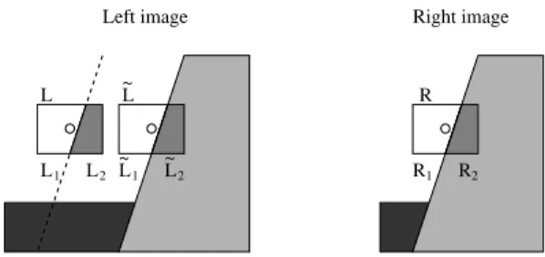
Correlation uses the assumption of constant depth within the correlation window. Depth variations introduce errors in the calculation. Whether the introduced error at a depth discontinuity can be neglected or leads finally to the wrong decision depends on the similarity between the object, the occluded and visible part of the background, which is cov-ered by the correlation window (figure 1).

L ~ L ~ 1 L ~ 2 L2 L1 R1 R2 L R Right image Left image

Figure 1: Typical decision conflict at object border. The correct corresponding position for the correlation window R would be L. It is necessary to split the correla-tion window into two halves to understand why it happens that sometimes the correlation of R with ˜L gives a higher response than R with L. This results effectively in an ex-tension of the object at its left border. Let cab be the

correlation value of the area a and b, where a low value corresponds to a high similarity. The values cR1L1 and

cR2L˜2 should be very low, because the corresponding

re-gions are correctly matched. The choice between the po-sition L and ˜L depends on the amount of similarity of R2

and L2and the similarity of R1and ˜L1. The areas L2and

˜

L1 are occluded in the right image. If cR2L2 is higher

than cR1L˜1

2_{, then the wrong position ˜L will be chosen.}

Image noise will affect the choice, but it depends mostly

2_{It needs to be considered, that the area R}

1is bigger in this example and

has a higher effect in the correlation process. However, a small amount of large errors can have a higher effect than a large amount of small errors, depending on the correlation measure.

on the similarity between the occluded background, visible background and object.

Usually, the background continues similarly and L1

would be similar to ˜L1 and L2 dissimilar to ˜L2. This

leads to the presumption that objects usually appear bigger. However, shadows or changing texture near object borders can inverse the situation, so that the object would become smaller. The same scenario can be drawn for right borders and leads to fuzzy, blurred object borders. Furthermore, top and bottom borders suffer from similar problems. However, the effect is expected to be less severe, since there is no oc-cluded area at top or bottom borders.

Generally, there may not only be one depth change in-side a correlation window, but it is a very common case, as surfaces vary usually smoothly within real images, except at object borders [8].

Table 1 shows the amount of errors near (i.e. within the size of a correlation window) object borders, using the stereo image set from the University of Tsukuba (figure 5). Correlation was performed using the Sum of Absolute Dif-ferences (see table 2). Disparities that failed the left/right consistency check [9] have not been considered. Only dis-parities that differ by more than one from the ground truth were treated as errors.

Border errors are categorised according to the kind of border and if the error identified the background wrongly as object (i.e. increased the size of the object) or identified the object wrongly as background.

Border Wrong Wrong Max. Factor

Obj. [%] Back. [%] Err. [%]

left 1.67 0.19 8.35 0.22

right 1.73 0.40 8.51 0.25

top 0.14 0.04 3.61 0.05

bottom 0.19 0.17 3.31 0.11

Table 1: Errors at borders, using SAD on Tsukuba images. The results show indeed that most errors occur at left or right object borders and extend objects horizontally. Fur-thermore, all cases of border errors can be explained, us-ing the theory above, by thorough visual analysis of the Tsukuba images and the resulting disparity image.

3. Multiple supporting windows

Correlation windows that overlap a depth discontinuity in-troduce an error into the correlation calculation. The error can be reduced by only taking those parts of a correlation window into consideration, which do not introduce errors. However, this has to be done systematically and compara-bly, as described below.

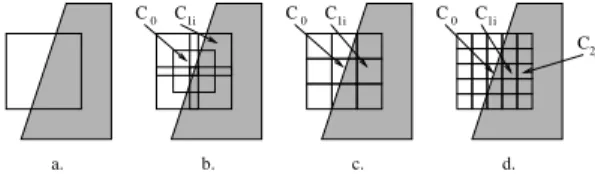
Figure 2b shows a configuration with one small window in the middle (C0), surrounded by four partly overlapping

windows (C1i). The correlation value C can be computed

by adding the values of the two best surrounding correlation windows C1i1and C1i2 to the middle one. This approach can

also be seen as using a small window C0and supporting the

correlation decision by four nearby windows. C C0

C1i1 C1i2 (1)

Another configuration using nine supporting windows is shown in figure 2c. The correlation value is in this case calculated by adding the four best surrounding correlation values to the middle one.

C C0

C1i1 C1i2 C1i3 C1i4 (2)

The approach can be extended by adding another ring of surrounding windows as shown in figure 2d. The eight best values of the outer ring are additionally added.

C C0

C1i1 C1i4 C1k1 C1k8 (3)

It can be seen that it is possible for these correlation win-dows to adapt to the local environment by assembling a big correlation window out of smaller ones. The blurring effect should be reduced as only the small middle window C0is

always used and may overlap the depth discontinuity. All other parts can adapt to avoid an overlap with the depth dis-continuity. Nevertheless, a good correlation behaviour is still maintained, because of the big area, which is covered using the best neighbouring windows. The measure for cal-culating the correlation value of the individual windows can be selected as needed. 0 C C_1i C₀ C_1i 2j C 0 C C_1i c. d. a. b.

Figure 2: Configurations with multiple windows. The computation of C seems to be computationally costly as it needs to be done for all image pixels at all possi-ble disparities. However, an implementation can make use of the same optimisations proposed for standard correlation [10] to compute the individual windows. Additionally, the best surrounding correlation windows have to be selected and a sum needs to be built. The selection of the best win-dows is costly, as it requires a sorting-like algorithm. Se-lecting the two best values out of four as required by the configuration with five windows can be implemented with four comparisons, while nine windows would require 16 comparisons and 25 windows even 80 comparisons. Conse-quently, the simple configuration using five windows seems suitable for a real time implementation.

4. Filtering of general errors

The determination of a disparity value involves correlating the window in the first image with windows at all dispari-ties d in the second image. The resulting correlation values C form a correlation function as shown in figure 3. The disparity at which the correlation function is lowest corre-sponds with the place of highest similarity3. The left/right consistency check [9] uses the place of highest similarity in the second image and then moves the correlation window of the first image over all possible disparities, which gives another correlation function. The disparity is considered to be valid if the minimum of the second correlation function corresponds to the same disparity as the minimum of the first correlation function.

C₂ C₁ c

d

Figure 3: A typical correlation function. The minima C1is

the place of highest similarity.

The left/right consistency check is a very effective mean to identify places where correlation is contradictory and thus uncertain. This is usually the case at occlusions [6]. An analysis of the correlation function can further help to identify uncertainties. A nearly flat correlation function cor-responds to areas with low texture. A function with several minima indicates several good places which can be caused by repetitive texture. Image noise can in these cases easily lead to wrong decisions. Let C1be the minimum correlation

value and C2the second lowest correlation value, which is

not a direct neighbour of C14. The relative difference Cdcan

be calculated as:

Cd

C2 C1

C1

(4) A low Cdindicates possible problems. It is assumed that

many errors will be caught by invalidating all values whose Cd is below a certain threshold for one of the correlation

functions (i.e. the correlation function for the left and right image, as used by the left/right consistency check as well). However, the threshold needs to be set empirically.

Moravec’s Interest Operator offers a way of invalidating areas with low texture before correlation is performed [12]. However, the method described above sees the image di-rectly through the eyes of the correlation function, which should be more accurate. Secondly, problems with repeti-tive like texture are treated at the same time.

3_{The SAD correlation responds with low values if the similarity is high.} 4_{The best place for correlation lies usually between pixels, so that}

5. Border correction filter

The behaviour of stereo correlation at object borders de-pends on local similarities. It was shown in section 2 that most errors appear at left and right object borders and ex-tend the size of objects. This is a systematic error that is typical for correlation. A correction of this error would im-prove the shapes of objects significantly.

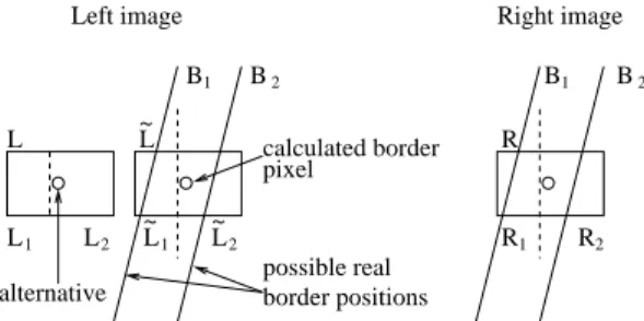
After the disparity image is calculated, vertical dispar-ity gradients can be discovered by comparing horizontally neighbouring disparity values. A positive disparity step rep-resents a calculated left object border, while a negative step represents a calculated right object border. The real position of the object border is usually within the distance of half the size of a correlation window, according to the theory in section 2. However, usually there are some filters used that invalidate some disparity values, like the left/right con-sistency check, which invalidates many occluded disparity values near left object borders [9]. For the purpose of iden-tifying disparity steps, the lowest neighbouring value of an invalidated area is propagated through the invalid area [6].

Figure 4 shows a situation of a positive disparity step. The dotted line marks the position of the calculated left ob-ject border5. The pixel of interest in the middle of the cor-relation window corresponds to the higher disparity of the object, while all pixels to its left have the lower disparity of the background. If the calculated border is correct, then only the correlation cR2L˜2 is correct for a correlation of

R with ˜L. The correct partner for R1would be L1, which

is shifted to the left by a distance that corresponds to the disparity difference between the object and the background. All pixels between the right border of L1and the left border

of ˜L2would be occluded. L ~ R2 R1 L ~ 2 L ~ 1 L2 L1 B2 B1 B1 B2 pixel calculated border R L

alternative border positions possible real

Left image Right image

Figure 4: Situation where ˜L has been chosen. This is cor-rect, if the real border is at B1, but wrong if it is at B2.

However, the real object border is usually a few pixels further left or right and in general not vertical. The direc-tion in which the real object border is, can be identified by comparing cR1L1 and cR2L˜2. To compare both values

properly, the size of both halves of the correlation window

5_{The calculated object border is assumed to go always vertical through}

the correlation window, for simplicity of calculation.

is made equal by increasing the left part by one pixel6. If the real border corresponds to position B1, then the value

cR2L˜2 should be low because it is completely correct,

while cR1L1 should be high because only a part of R1

does really correspond to L1. The situation is vice versa if

the real position of the border corresponds with B2. Finally,

if the position of the real border goes through the middle of the correlation window, both correlation values are equally low apart from image noise.

Consequently, the values cR1L1 and cR2L˜2 are

cal-culated, while moving the windows in both images simulta-neously to the left and right. The position where both values swap places in terms of their amount is searched. Finally, the position where cR1L1

c

R2L˜2 is lowest is chosen

as the correct position of the object border. The disparity values need to be corrected accordingly.

The depth might vary not only once in practise, but sev-eral times within a small area. This violates again the as-sumption of constant depth within half of a correlation win-dow. However, the case above is assumed to occur often and thus justifies this special treatment.

The computational expense is low compared to the cor-relation stage, because only places where object borders are assumed need to be inspected. Processing the Tsukuba stereo image pair results typically in less than 5% of the pixels, which are assumed object borders. This includes all errors, which introduce false borders as well.

The border correction algorithm requires the calculated disparity image as well as both source images and the size of the correlation window as input.

Go line by line, left to right through the disparity.

– Interpolate invalid values, by using the lowest

neighbour in horizontal direction.

– Identify a positive disparity step, i.e. a low

dis-parity value followed by a higher one.

– Calculate cR1L1 and cR2L˜2 at the position

of the disparity step.

– If cR1L1 is higher than cR2L˜2, then

Analyse the next pixel to its left and assign the object disparity to it if cR1L1 is higher

than cR2L˜2 or if cR1L1

c

R2L˜2 is

lower than the same value for last position (i.e. the pixel to its right).

Continue to move pixel-wise to the left until cR1L1 is lower than cR2L˜2 or the

max-imum range (i.e. half the size of the correla-tion window) has been covered.

– else

6_{Correlation windows have commonly an odd size so that they are}

Search the border to the right, analog to the algorithm above.

Do the same to correct all right object borders analog to the algorithm above.

6. Summary of the whole algorithm

The improvements, which have been suggested in the last sections can be included into the framework of a standard correlation algorithm. The source images are expected to be rectified, so that the epipolar lines correspond with image rows.

1. Pre-filtering source images as needed, using LOG. The standard deviationσcontrols smoothening.

2. Correlate using a configuration with one window, five, nine or 25 windows as described in section 3. An opti-mised calculation of correlation values is required for real time applications [10]. The kind of correlation measure needs to be chosen (e.g. SAD). Parameters are the width and height of the correlation window cw

and ch.

3. The left/right consistency check invalidates places of uncertainty [9]. It can effectively be implemented by temporarily storing all correlation values of all dispar-ities for one image row.

4. The error filter can be used to reduce errors further, as described in section 4. The threshold tf is needed as a

parameter.

5. The border correction may be used in the end to im-prove the disparity image as described in section 5.

7. Results on real images

7.1. Experimental setup and analysis

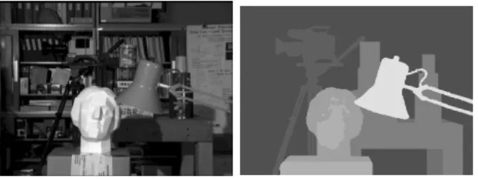
A stereo image pair from the University of Tsukuba (figure 5) and an image of a slanted object from Szeliski and Zabih [11] have been used for evaluation. Both are provided on Szeliski’s web-page7_{. The image of the slanted object is}

very simple. However, it is expected to compensate for the lack of slanted objects in the Tsukuba images.

All disparities that are marked as invalid during the cor-relation phase have been ignored for comparison with the ground truth. Disparities that differ by only one from the ground truth are considered to be still correct [11]. The amount of errors at object borders is calculated as explained in section 2 and shown separately.

7_{http://www.research.microsoft.com/˜szeliski/stereo/}

The difference images, which are provided next to the disparity images show the enhanced difference of disparity and ground truth. Correct matches appear in medium gray, while darker spots indicate that these pixels are calculated as being further away as the ground truth states. Whereas light spots show that those pixels are calculated as being too close.

Figure 5: The left image and the ground truth from the Uni-versity of Tsukuba.

The range of possible disparities has been set to 32 in all cases. For every method, all combinations of meaningful parameters were computed to find the best possible combi-nation for the Tsukuba images. The horizontal and vertical window size was usually varied between 1 and 19. The stan-dard deviation of the LOG filter was varied in steps of 0.4 between 0.6 and 2.6. All together almost 20000 combina-tions were computed for the Tsukuba image set, which took several days using mainly non-optimised code.

7.2. Results of standard correlation methods

The results of the best parameter combination (i.e. which gives the lowest error) for some standard correlation meth-ods can be found in the first part of table 2. The MW-SAD approach performs correlation at every disparity with nine windows with asymmetrically shifted points of interest and uses the best resulting value. Algorithms, which are based on this configuration have been proposed in the literature for improving object borders [6].

The best parameter combinations of the Tsukuba images have been used on the slanted object images as well. Al-most all errors occur near object borders on this simple im-age set. This is probably due to the evenly strong texture and the lack of any reflections, etc. It is interesting that the slanted nature of the object, which appears as several small depth changes, is generally well handled. However, the weak slant is not really a challenge for correlation. The results are not explicitely shown here, because they reflect the same tendency as the results of the Tsukuba images, es-pecially there ordering. However, it is a confirmation of the qualitatively correct assessment of the evaluated methods.

The SAD correlation (figure 6) was chosen as the basis for an evaluation of the proposed improvements. It is the fastest in computation and shows advantages over NCC and

Method Window Rank / Census LOG σ Correct [%] All Errors [%] Border Err. [%] Invalid [%]

Normalised Cross Correlation (NCC) 9 x 19 - 0.0 82.37 8.15 7.05 9.49

Sum of Absolute Differences (SAD) 9 x 9 - 1.0 82.97 6.00 4.39 11.03

Sum of Squared Differences (SSD) 9 x 9 - 1.0 81.42 6.55 4.88 12.03

Non-parametric Rank 11 x 11 9 x 7 - 85.68 4.58 3.96 9.74

Non-parametric Census 9 x 11 9 x 7 - 84.86 4.65 3.87 10.49

SAD with mult. windows (MW-SAD) 11 x 9 - 0.0 80.88 4.91 2.92 14.21

SAD with 5 windows configuration 7 x 9 - 0.0 85.12 4.56 3.36 10.32

SAD with 9 windows configuration 5 x 5 - 0.0 83.65 4.39 2.89 11.96

SAD with 25 windows configuration 3 x 5 - 1.0 83.36 4.89 3.36 14.67

SAD with Border correction 9 x 9 - 1.0 85.63 6.10 4.04 8.26

SAD with 5 windows configuration and 10% error filtering

7 x 9 - 0.0 80.70 3.02 2.59 16.28

SAD with 5 windows configuration, 10% error filtering and border corr.

7 x 9 - 0.0 82.24 3.26 2.45 14.50

Table 2: Results of standard methods (first part), suggested improvements (second part) and combinations (third part) on Tsukuba images.

SSD. It was therefore chosen for other real time stereo sys-tems as well [1] [2]. The non-parametric Rank and Census transform give better results, because they are more tolerant against outliers [5]. However, Census is expensive to com-pute due to the calculation of the Hamming distance and Rank is rather seen as a filter, like LOG, that transforms the source images before a SAD correlation is performed.

7.3. Results of suggested improvements

All suggested improvements have been evaluated using SAD correlation. The results of the best parameter combi-nations are shown in the second part of table 2, except error filtering, which is presented in figure 10. Border correction was only applied to the best parameters of SAD.

The multiple correlation window configuration showed improvements in the number of correct matches as well as errors. The performance seems to be especially good at ob-ject borders. Figure 7 shows the results from the five win-dows configuration. The rings of errors around objects look smaller and more even, compared to figure 6. A comparison with the MW-SAD method shows a more stable behaviour. MW-SAD shows better results in the synthetic case of hor-izontal or vertical borders, but performs worse at general border shapes. Additionally, it is far less stable in general, which increases general errors as well as invalid matches.

The error filter that was tested for different thresholds on the best parameter configuration of SAD exhibits an ex-pected characteristic. The graph in figure 10 shows that many errors can be caught at the risk of filtering correct matches out as well. However, the amount of filtered errors compared to filtered correct matches is quite high when the

ratio between errors and correct matches is considered. A threshold of 10% filters for example almost 2% errors out, at the expense of loosing 4% correct matches. Furthermore, filtered correct matches are distributed all over the image, so that there disappearance can be compensated by inter-polation. In the end, it depends on the application, which amount of lost correct matches is acceptable.

filtered correct matches filtered border errors filtered other errors [%] 5 10 15 20 0 0 4 8 threshold [%]

Figure 10: Filtered correct matches and errors at certain thresholds, using SAD on the Tsukuba images.

The threshold for error filtering is difficult to choose. One strategy in practise (i.e. without having a ground truth) could be to set the threshold so that the number of invalid matches is increased by a fixed amount.

Finally, an evaluation of the border correction shows only a slight decrease in errors at object borders and an un-expected increase of errors at other places. Nevertheless, the number of correct matches is in this example increased by 2.66%. The situation can be explained using figure 8. The borders of objects are in fact improved compared to figure 6, which results in the decrease of border errors. The increase in correct matches results from changing many in-valid values near object borders into in-valid, correct values.

Figure 6: Result from SAD correlation.

Figure 7: Result from the five window configuration.

Figure 8: Result from SAD correlation with border correction.

The increase in errors at other places is due to the fact that the algorithm tried to correct object borders that resulted from previous errors, leading to a randomly stretching or shifting of error patches. The white spots left to the camera and on the top left edge of the image are good examples of this behaviour.

Although, borders are improved, small details which were lost during the correlation phase, like the cable of the lamp, can not be recovered using this method. Finally, it can be concluded that the effect of noise gets stronger, the fur-ther the border is moved towards the real object border, due to the design of the calculation. This leads to the reduced, but still existent amount of border errors.

The third part of table 2 shows results of combinations of several methods. The best parameter combinations estab-lished previously have been used. The result is also shown in figure 9. Comparing these results visually and in their statistical numbers against any of the standard correlation methods shows clearly a significant improvement for cer-tain applications. The error values were cut to half of their amount of basic SAD correlation.

8. Conclusion

It has been shown that it is possible to improve simple cor-relation by understanding the source of its weakness. Three methods have been proposed, which tackle specific prob-lems of correlation. A novel multiple window approach decreases errors at object borders and increases correct matches. A general error filter uses the correlation function to invalidate uncertain matches. Finally, a border correction method improves object borders further in a post-processing step. It was discussed that all improvements are still suitable for real-time applications.

Every method shows clear improvements, but also weak-nesses. The main weakness of the multiple correlation window configuration is its computational cost. However, the configuration using five windows seems very promis-ing. The error filtering requires a threshold, which is diffi-cult to choose in practise and reduces the number of cor-rect matches as well. Finally, the border corcor-rection im-proves object borders, although previous general errors can be slightly increased.

Nevertheless, the combination of suggested methods im-proves the quality of real-time correlation based stereo sig-nificantly. The errors have in the example images been reduced to 50%, while the number of correct matches has been maintained. Further research in this area could bring even better real-time results on current computer hardware. The current implementation has been written for qualita-tive assessment and has not been optimised. It is planned to implement a real time system as the basis for a higher level, object based processing to support tele-operated tasks.

Acknowledgements

I would like to thank DERA for their financial support, Dr. Peter Innocent and Dr. Jon Garibaldi for their advice and the University of Tsukuba and R. Szeliski and R. Zabih for their stereo images with ground truth.

References

[1] K. Konolige, “Small vision systems: Hardware and imple-mentation,” in Eighth International Symposium on Robotics

Research, (Hayama, Japan), pp. 203–212, London, Springer,

October 1997.

[2] L. Matthies, A. Kelly, and T. Litwin, “Obstacle detection for unmanned ground vehicles: A progress report,” in

In-ternational Symposium of Robotics Research, (Munich,

Ger-many), October 1995.

[3] T. Kanade and M. Okutomi, “A stereo matching algorithm with an adaptive window: Theory and experiment,” IEEE

Transactions on Pattern Analysis and Machine Intelligence,

vol. 16, p. 920, September 1994.

[4] R. Zabih and J. Woodfill, “Non-parametric local transforms for computing visual correspondance,” in Proceedings of the

European Conference of Computer Vision 94, pp. 151–158,

1994.

[5] Y. Boykov, O. Veksler, and R. Zabih, “A variable window ap-proach to early vision,” IEEE Transactions on Pattern

Anal-ysis and Machine Intelligence, vol. 20, December 1998.

[6] A. Fusiello, V. Roberto, and E. Trucco, “Efficient stereo with multiple windowing,” in Proceedings of the Conference on

Computer Vision and Pattern Recognition, (Puerto Rico),

pp. 858–863, IEEE, June 1997.

[7] J. J. Little, “Accurate early detection of discontinuities,”

Vi-sion Interface, pp. 97–102, 1992.

[8] D. Marr and T. Poggio, “A computational theory of human stereo vision,” Proceedings of the Royal Society, vol. B-204, pp. 301–328, 1979.

[9] P. Fua, “A parallel stereo algorithm that produces dense depth maps and preserves image features,” Machine Vision

and Applications, vol. 6, pp. 35–49, Winter 1993.

[10] O. Faugeras, B. Hotz, H. Mathieu, T. Viville, Z. Zhang, P. Fua, E. Thron, L. Moll, G. Berry, J. Vuillemin, P. Bertin, and C. Proy, “Real time correlation-based stereo: algorithm, implementations and application,” Tech. Rep. 2013, INRIA, August 1993.

[11] R. Szeliski and R. Zabih, Vision Algorithms: Theory and

Practice, ch. An Experimental Comparison of Stereo

Algo-rithms, pp. 1–19. Corfu, Greece: Springer-Verlag, Septem-ber 1999.

[12] H. Moravec, “Toward automatic visual obstacle avoidance,” in Proceedings of the Fifth International Joint Conference

on Artificial Intelligence, (Cambridge, MA), pp. 584–590,