Vol. 1, Nos. 1-2, pp 79-109
Parametric and Nonparametric Regression with
Missing
X
’s—A Review
Helge Toutenburg, Christian Heumann, Thomas Nittner, Sandro Scheid
Department for Statistics, Ludwig–Maximilians–University Munich, Lud-wigstr. 33, 80539 Munich, Germany.
([email protected], [email protected], [email protected], [email protected])
Abstract. This paper gives a detailed overview of the problem of missing data in parametric and nonparametric regression. Theoreti-cal basics, properties as well as simulation results may help the reader to get familiar with the common problem of incomplete data sets. Of course, not all occurences can be discussed so this paper could be seen as an introduction to missing data within regression analysis and as an extension to the early paper of [19].
Received: September 2002
Key words and phrases: Generalized additive models, imputation, missing data mechanism, MSE–superiority, regression analysis.
1
Introduction
Statistical analysis with missing data is a common problem in prac-tice. Nonresponse in sample surveys or drop–out in clinical trials may be two of many examples one could imagine. Apart from the esti-mation of sample statistics regression analysis as a main tool within statistical analyses of dependencies therefore often is affected by miss-ing values, too. Whereas parametric regression has been investigated extensively, nonparametric methods haven’t been considered within this context so far. Apart from the standard literature concerning missing data, i.e., [20] and [26], linear regression (e.g. [19]), logistic regression (e.g. [40]) and generalized linear models (e.g. [18]) were considered within the scope of parametric methods. Little emphasis has been put on nonparametric regression analysis—e.g., [7] or some simulation experiments by [22].
Before defining the basic terms and relations within the context of missing data, the parametric as well as the nonparametric regression model is introduced.
1.1 Linear Regression Models
Assume the linear regression model
Y =X1β1+. . .+Xpβp+ (1)
and its sample version
y=Xβ+ (2)
whereyis the (n×1)–vector of observations of the dependent variable,
X is the (n×p)–matrix of the independent regressiors and is the (n×1)–vector of disturbances. We confine ourselves to nonstochastic
X and assume X to be of full column rank. Further let
∼(σ2, In) (3)
or
∼N(σ2, In) (4)
for testing hypothesis. IfX is complete, the BLUE of β is given by
b= (X0X)−1X0y. (5) In statistical practice, however, we often have incomplete data— marked by ‘∗’— in the response y as well as in the data matrix, i. e.
(yX) =
y1 x11 · · · x1p
y2 ... ∗ ...
∗ ∗
..
. ... ∗ ...
yn xn1 · · · xnp
(6)
In general, we may assume the following structure of the data which is discussed in full detail in [24], Chapter 6,
yobs
ymis
yobs∗
=
Xobs
Xobs∗ Xmis
β+ . (7)
Estimation of ymis corresponds to the prediction problem. Based on these results, we may confine ourselves to the substructure
yobs
yobs∗
= Xobs Xmis
β+ (8)
of (7) and change the notation as follows:
yc y∗ = Xc X∗ β+ c ∗ , c ∗
∼(0, σ2I). (9)
The submodel
yc =Xcβ+c (10)
stands for the completely observed data (c : complete), and we have
yc : m × 1, Xc:m × p, and rank(Xc) =p.
The other submodel
y∗=X∗β+∗ (11)
is of dimension (n−m) =J. The vectory∗is observed completely. In
the matrix X∗ some observations are missing. The notationX∗ will
underline that X∗ is partially incomplete, in contrast to the matrix
Xmis, which is completely missing. Combining both of the submodels in model (9) corresponds to the so–called mixed model ([32]). There-fore, it seems to be natural to use the method of mixed estimation.
1.2 Generalized Additive Models
Generalized Additive Models (GAM) became more and more popular since the work of [16]. One could consider GAMs as the generalization of linear as well as generalized linear models and, of course, additive models. Its flexibility concerning the modelling of the functional re-lation build the main advantage over linear models and generalized linear models (GLM) based on the a priori unknown function f(X) which has, for example, to be specified within polynomial regression when the purpose is a non–linear relation between y and X.
Before introducing the GAM a short summary is given to generalized linear models to get familiar with the necessary terms. Following the notation within the previous section the observations yi are assumed
to be independent identically distributed with µi = E(yi), the mean
given byµi =x0iβ. GLMs may then be described by
1. thedistribution assumption which postulates the yi to be
con-ditionally independent of the xi with the conditional
distri-bution of yi belonging to a simple exponential family with
µi= E(yi |xi) and a scaling parameter φ.
2. thestructural assumption which relates µi with the linear
pre-dictorηi =x0iβ according to
µi =h(ηi) =h(x0iβ), resp. ηi=g(µi), (12)
with the one–to–one known function hand g being the inverse function of h called link function.
Following [12] a generalized linear model is characterized by the type of the exponential family, the link function, and the design vectorxi.
Generalized additive models differ from generalized linear models by assuming an additive predictor instead of a linear predictor and are defined by
g(µ) =α+
p
X
j=1
fj(Xj), (13)
with an appropriate link function. Partition (8) and, especially, the distribution of the errors noted in (9) are assumed to hold here, too. The mixed estimator within this context can not be written in such
a way which forces us to introduce the inference within GAMs just in general.
Similar to the minimization of the target function within the linear model we formulate a target function with respect to the smoothness of f(x) according to
n
X
i=1
{yi−f(xi)}2+λ
Z
f00(x)2dx , (14)
which is to be minimized with respect to the parameters of f(x). f0
and f00 have to be continuous,f00 has to be quadratically integrable.
λcontrols the trade–off between variance and bias well known from a simple scatterplot smoother. λ→ ∞ equals a straight line, λ= 0 leads to an unsmoothed estimate ˆf(xi) =yi meaning a reproduction
of the data, see [39].
The estimation is done byiteratively re–weighted least squares(IRLS) where each least–squares step is replaced by a penalized one. The cri-terion is the maximization of the penalized loglikelihood
lβ =λ n
X
i=1
li(yi, Xiβ)−
1 2
m
X
i=1
θiβ0Siβ , (15)
wheremquadratic penalties are to be applied to the parameter vector
β. The matrix Si contains the penalties which imply each smoothing
parameter θi. β(k) is estimated by Fisher–Scoring Algorithmus, see
Table 1.
β(k+1) = β(k)+ E[− δ2lβ δβ(k)δβ(0k)]
−1 δlβ
δβ(k) respectively,
β(k+1) = β(k)+ [X0W(k)Xλ+P
θiSi]−1{X0W(k)Γ(k)(y−µ(k))−P
θiSiβ(k)}
Table 1: Fisher–Scoring.
Wii(k) = g0(µi(k))Vi−1 is a weighting matrix, Vi is the variance of y
with respect toµ(ik); Γii=g0(µ(ik)). g(µi) is a monotone link function.
Following [43], the determination ofβ(k+1) within f with E(f(Yi)) =
1. By the help ofβ(k)one gets estimates forµand the variancesVi for eachyi; compute
(i) the diagonal matrix of weightsW with Wii= (g0(µi)2Vi)−1
(ii) the vector
z=Xβ+ Γ(y−µ) ,
a vector of pseudo data with the diagonal matrix Γii= (g0(µi))−1
2’. Computeλi by minimizing
||W12(z−Xβ)||2
(sp(I−A))2
withβ being the solution of minimizing
||W12(z−Xβ)||2+Pλjβ0Sjβ
with respect toβ andA being the hat–matrix with A=X(X0W X+Pλ
jβ0Sjβ)−1X0W .
Table 2: IRLS with GCV.
f(β) is equivalent to solving the weighted penalized least squares problem
minλ||W12(z(k)−Xβ)||2+Xθiβ0Siβ (16)
with a pseudo data vector z(k) = Xβ(k)+ Γ(k)(y−µ(k)), the global smoothing parameter λ, the diagonal matrix of weights W and the nonnegative definite matrix S of coefficients containing the penalty terms θi for the smoothing parameters. (16) in practice is solved by
minimizing the generalized cross validation (GCV) scores
V = ||W
1
2(y−A(λ, θ)y)||2/n
[1−tr(A(λ, θ))/n]2 (17)
with respect to θiλ. ˆµ =Ay holds for the hat–matrix A. Combining IRLS and GCV represents the algorithm of interest, illustrated in Table 2 (see [14] or [43]).
Note that the degrees of freedom is an integrative part of the estima-tion. An extensive description of estimating GAMs can be found in [39].
2
Missing Data Pattern and Missing Data
Mechanism
So far, we introduced just methods and assumptions analyzing the data set as it is. Because of the effects of the missingness, i.e. the amount of missing values, on the data structure and, therefore, the amount of information the analyst has to deal with these problems. The missing data pattern and the missing data mechanism are two important terms visualizing and characterizing the situation of the data.
2.1 Missing Data Pattern
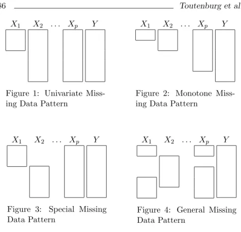
As already mentioned above, visualizing the structure of the data set with respect to the missing values may be a first way to get an impression of the situation. Also implemented in statistical software, the missing data pattern do a good job; the observed cases of a vari-able correspond to one bar—the more missing values, the shorter the bar of the variable, see Figures 1–4. Figure 1 shows the situation when one variable is incomplete and all other variables are completely observed—a special case of the monotone pattern in Figure 2 where each variableXj is observed for at least the cases ofXj−1. An exam-ple for a special pattern is shown in Figure 3 where X2 is observed for the cases where X1 is missing and vice–versa. This is a common problem known as double sampling, see [26]. Figure 4 illustrates a situation with no special structure.
Although the missing data pattern represent an easy way to get a first impression, more complex dependencies between observed and incomplete variables or incomplete variables themselves will reduce this ability strongly. This is one reason why the missing data mech-anism has to be considered.
2.2 Missing Data Mechanisms (MDM)
The main question within the context of analyzing incomplete data sets is whether the missing data mechanism can be ‘ignored’—a term
X1 X2 . . . Xp Y
Figure 1: Univariate Miss-ing Data Pattern
X1 X2 . . . Xp Y
Figure 2: Monotone Miss-ing Data Pattern
X1 X2 . . . Xp Y
Figure 3: Special Missing Data Pattern
X1 X2 . . . Xp Y
Figure 4: General Missing Data Pattern
which is to be specified—or not. One could make the assumption that the mechanism is ignorable in the sense described below; the other possibility consists of including the missing data mechanism—which still is to define—in the statistical model. Including the MDM means including the distribution of an indicator variable R indicating if a component of the data matrix Z is observed or missing. [20] define the data matrix Z = (Zobs, Zmis) representing the data that would occur without missing values. The random variableR indicating the missingness within the data matrixZ is defined according to
rij =
1 if zij observed
0 if zij missing
∀i= 1, . . . , n, j = 1, . . . , p+ 1. (18)
The question whether the missing mechanism can be ‘ignored’ for the estimation of θ equals the question whether statistical inference is based on the density f(Zobs, R|θ,Φ)—with Φ being an unknown parameter of the missing mechanism and θ being the parameter of the density of Zobs, Zmis—or on the simpler density f(Zobs, θ) which is ‘ignoring’ the missing mechanism. The classification of the missing data mechanism is based on the densityf(R|Zobs, Zmis,Φ) and leads
to the definition of
1. MCAR (missing completely at random) if
f(R|Z,Φ) =f(R|Φ) ∀Z , (19)
2. MAR (missing at random) if
f(R|Z,Φ) =f(R|Zobs,Φ) ∀Zmis,and (20)
3. MNAR (missing not at random)
f(R|Z,Φ) =f(R|Zobs, Zmis,Φ). (21)
Following [20], the missing data mechanism is said to be ignorable in the context of likelihood inference when the distribution of the miss-ing mechanism is independent of the missmiss-ing values [(20)] themselves. This may be more apparent by computing the density of the actual observed data obtained by integrating Zmis out of the density
f(Zobs, R|θ,Φ) = Z
f(Zobs, Zmis|θ)f(R|Zobs, Zmis,Φ)dZmis (22)
which by help of (20) leads to
f(Zobs, R, θ,Φ) = f(R|Zobs,Φ) Z
f(Zobs, Zmis, θ)dZmis = f(R|Zobs,Φ)f(Zobs |θ). (23)
The likelihood–based inferences forθ based on f(Zobs, R|θ,Φ) and for θ based on f(Zobs | θ) are the same if the parameters θ and Φ concerning the density ofZand the missing mechanism, respectively, are distinct in the sense of each parameter containing no information about the other (see for example [26]).
3
Inference and Missing Data
3.1 The Mixed Model with Missing Regressor Values
Following the concept of missing values introduced by [20] leads to a partition of the sample (y1, . . . , yn) in two samples, the first contains
all thoseyi with completely givenxi–vectors (saym < nelements of
the sample).
yc =Xcβ+c (subscriptc: complete). (24)
In general we assume Xc to be of full column rankp.
The second sub–sample contains all those yi where the associated
x–rows are partially or fully unknown (sayJ elements of the sample,
m+J =n).
y∗=X∗β+∗, ∗∼(0, σ2IJ). (25)
That is,yc, y∗andXcare known, butX∗is partially or fully unknown.
Combining (24) and (25) gives the mixed model
yc
y∗
=
Xc
X∗
β+
c
∗
.
c
∗
∼(0, σ2In). (26)
The optimal but due to the unknown elements ofX∗ not operational
estimator (BLUE) of β is given by the mixed estimator (cf. [24], Ch. 5)
ˆ
β(X∗) = (X
0
cXc+X
0
∗X∗)−1(X
0
cyc+X
0
∗y∗)
= bc+Sc−1X∗0(IJ+X∗Sc−1X∗0)−1(y∗−X∗bc) (27)
having the covariance matrix V( ˆβ(X∗)) =σ2(X
0
cXc+X
0
∗X∗)−1 =σ2(Sc+S∗)−1 (28)
where S∗ = X
0
∗X∗ and Sc = X 0
cXc and bc = (Xc0Xc)−1Xc0yc is the
OLSE in the complete case submodel (24).
3.2 Common Missing Values Procedures 3.2.1 Complete Case Analysis
The first (and in many situations most obvious) method to obviate the problem of an incompletely observed design matrix results in resigning the incomplete model (25). This so–called classical LSE of β makes use of the completely observed design matrix Xc, only.
That is, the classical LSE (CLSE) estimatesβ from the model (1.2) according to
bc = (X 0
cXc)−1X 0
cyc (29)
having
V(bc) =σ2(X 0
cXc)−1=σ2Sc−1. (30)
The CLSE discards the partial information contained in y∗ and the
observed elements ofX∗ of the incomplete model (25). This may lead
to a loss in efficiency compared with estimators using a “repaired” version of model (25) whereas repairing means to fill the gaps inX∗
by some substitution method, for example.
3.2.2 Available Case Analysis
These methods estimateβ from normal equations (see [15]) according to
cov(xixj) ˆβ = cov(xiy) (i, j= 1, . . . , p), (31)
where cov(xixj) is thep×pcovariance matrix with the (i, j)th element
(i, j = 1, . . . , p) computed from the observations common to both
xi and xj(i 6= j) as well as from all existing measurements on xi
for i = j. Similarly, cov(xiy) is computed from all measurements
common to bothxi and y(i= 1, . . . , p).
¿From (31) we arrive at
cov(xixj)E( ˆβ) = E{(nij/niy)cov(xixj)β+ cov(xi)} (32)
and hence at
E( ˆβ) = (cov(xixj))−1{(nij/niy)cov(xixj)}β (i, j= 1, . . . , p).
(33)
nij and niy are the numbers of measurements common to both xi
and xj, and xi and y, respectively, minus unity. So β is unbiased
only when all niy’s are equal. Similarly, V( ˆβ) corresponds to the
CLSE form when nij =niy =njy(i, j= 1, . . . , n). In a Monte–Carlo
experiment for various patterns of missing observations [15] came to the conclusion that in most cases the complete case estimator is superior to the available case estimator.
3.2.3 Imputation by Zero–Order–Regression (ZOR)
By this method ([42]), which is also called unconditional mean im-putation, missing values xij of the jth regressorXj are replaced by
the sample (column) mean ˆxij of the observed values of Xj. This
method is expected to be convenient if the span or the range of the
Xj–realizations is moderate. It may fail in cases where the sample
mean is not a satisfactory representative of the missing sample ele-ments of Xj. This happens for example if trending time series or
growth curves are the laws generating the Xj–values.
The replacement of the missing xij–values in X∗ by ˆxij transforms
the (partially or fully unknown) matrixX∗into a known matrixX(1). Thus we are led to the operational model of mixed regression type
yc
y∗
=
Xc
X(1)
β+
c
(1)
, (34)
where the error term
(1)= (X∗−X(1))β+∗ (35)
has
(1)∼ {(X∗−X(1))β, σ2IJ}. (36)
[17] describe a version of this method, the so–called modified zero– order–regression.
3.2.4 Imputation by First–Order–Regression (FOR)
By this notion there is understood a complexity of methods to esti-mate missing elements ofX∗. In principle one constructs an auxiliary
regression
xij =θ0j+ p
X
µ=1 µ6=j
xiµθµj+uij, i6∈Φ = p
[
j=1
Φj, (37)
(uij : error term), Φj being the index set of missing values in xj, to
estimate the dependence between Xj(j = 1, . . . , p, jfixed) and the
other regressors X1, . . . , Xj−1, Xj+1, . . . , Xp. The missing value xij
then is estimated by ˆ
xij =θ0j+ p
X
µ=1 µ6=j
xiµθˆµj , (i∈Φj). (38)
(For examples compare [35].)
To overcome the difficulty caused by overlapping index sets, there are proposed certain methods depending on the pattern of missing values and on perceptible laws in the design matrix. [1] mentioned some averaging procedures (see also [3]).
Another possibility is to use the auxiliary regression with the high-est measure of determination whereas remaining missing values are replaced by other estimates, e.g., the corresponding sample means. [9] proposed a generalized LSE procedure, where the matrix Xc is
completed by first–order regression approximations.
[38] investigated some different procedures based on the FOR within a linear regression model with an incomplete binary covariate. The so–called pi imputation—simply imputing the probabilities based on the estimates of the logistic regression model—in terms of the empi-rical mean squared error showed good results.
An extension to the FOR in the context of generalized additive mo-dels could lead to an auxiliary regression which is also of the GAM type.
3.2.5 Imputation by Modified First–Order–Regression (MFOR)
The first order regression doesn’t use the responsey for imputing the missing data which is the idea of the modified first order regression (MFOR). Within the auxiliary regression model additionally the com-pletely observed response vector is used to predict the missing values. [3] considered this situation within the context of estimating µ and Σ in the normal model of (y, X1, . . . , Xp). [36] did some work on the
asymptotic properties of the MFOR estimates.
Regression parameters are biased when imputing for missing data using the MFOR. The early work of [1] provides some bias adjust-ment for the univariate case. The reason for the biased estimates lies in the inversion of the regression direction.
In [38] also a MFOR was compared to some alternatives concerning an incomplete binary variable; the estimates showed the expected larger variances resulting from the use ofy.
3.2.6 Multiple Imputation
In this paragraph we will describe the main ideas of the multiple im-putation. For details see for example [26] or [25].
So far, we imputed values that are a ‘good’ fitting to the data, ta-king into account either only the variable where missingness occurs, or additionally other variables. A problem that will occur is that the empirical variances of the variables will reduce and in the case of first order or modified first order regression association will be higher that they actually are.
Instead of imputing a ‘best’ value, draw values for the missing values, from conditional distributions that consider the uncertainty due to the prediction. The uncertainty arises from a distribution assump-tion and from the fact that parameter estimates themselves have variances. In contrast to the former methods, we will not only pro-duce one complete dataset, but draw several ones, that vary in the imputed values. The variation over the datasets may now reflect the uncertainty due to imputation.
First, distribution assumptions for the covariates where missing val-ues may occur have to be made. Together with the error distribution and the model equation we obtain a common distribution
PΘ(y, Xmis |Xobs), (39)
whereXmis denotes all covariates where missingness may occur,Xobs denotes completely observed covariates that depend on the parame-ters Θ, including the variance of the errors.
The method we will use to do multiple imputations is called data augmentation. As data augmentation is a Bayesian procedure one has to choose an appropriate prior distribution for the parameters Θ. For choices see e.g. [2].
Altogether we obtain
P(y, Xmis,Θ|Xobs) =PΘ(y, Xmis|Xobs)P(Θ). (40) Dependent on the distribution assumptions, we are able to draw data from the conditional distributions either directly or using sampling methods like MCMC.
Having chosen the first imputations for the missing values data aug-mentation consists of two steps that are applied consecutively many times until we can assume that the joint distributuion of the missing values and of the parameters Θ converge.
The steps are:
1. Imputation Step: For every row of the data set where missing values occur, draw from
P(Xmis|y, Xobs,Θ), (41)
and impute the drawn values as new values. Xmis denotes the covariates where missing values occur andXobs denotes the ob-served covariates.
2. Propability Step: Using the completed data set draw from
P(Θ|y, X1, ..., Xk) (42)
and take the drawn values as new parameter values.
Applying this procedure leads to several completed data sets. As-sume that we have drawn M data sets we now obtain the following estimators using estimates of the single data sets.
Letqbt, t= 1, ..., M be point estimates for theM completed datasets,
andcUtbe the variance estimate of the estimatorqbt. As new estimates
we obtain:
b
q= 1
M
M
X
t=1 b
qt, (43)
see [26].
c
Vqb= 1
M
M
X
t=1 c
Ut+ M
X
t=1
(qbt−bq)(qbt−qb)
0 (44)
The formulas above can be applied to scalar as well to multivariate estimators and will in our context in general be the estimates of our parameter vectorβ.
3.2.7 Nearest Neighbor Imputation
The nearest neighbor imputation has a long history but according to [6] is still not fully investigated although it is used in many surveys. Assuming the data structure withJ missing values for the row indices
i=n−J + 1, . . . , n visualized by
x1, . . . , xn−J
| {z } observed
, xn−J+1, . . . , xn
| {z }
missing
and
(45)
y1, . . . , yn−J, yn−J+1, . . . , yn
| {z }
observed
, (46)
a missing value xj, j=n−J+ 1, . . . , n, is imputed by choosing that
value xi, 1 ≤ i ≤ n−J, which is the nearest neighbor of j. In
this context the distance determining the nearest neighborhood is measured iny–values such thatisatisfies
|yi−yj | = min1≤l≤n−J |yl−yj | . (47)
If the solution is not unique the mean of the correspondingx–values may be imputed.
The nearest neighbor imputation is a hot deck imputation procedure which yields values unlikely to be nonsensical. Population means and quantiles are asymptotically unbiased and consistent (see [5]). Since it is a nonparamteric method it is expected to be somewhat more robust against model violations. [6] give a detailed overview over several possibilities for adjusting the procedure in order to get asymptotically unbiased and consistent variance estimates.
[22] investigated a simple additive model with missing completely
at random in the covariate and came to the result that the near-est neighbor imputation showed results similar to the complete case analysis—a procedure with best asymptotic properties when the miss-ingness is independent ofy. A forthcoming work considers the situa-tion when the missingness depends ony; first results showed that the CCA became worse and the nearest neighbor imputation still shows good results.
3.2.8 ML Estimation of the Missing Values
Let us now assume that the disturbances are normally distributed,
c ∼N(0, σ2Im), ∗ ∼N(0, σ2IJ). (48)
Handling the nonobseved regressor values like unknown parameters which have to be estimated common withβandσ2leads to the follow-ing considerations. For reasons of simpler mathematical presentation we confine ourselves to models without a constant and to the case of a fully nonobserved regressor matrix X∗ which has to be estimated
from the model
yc
y∗
=
Xc
X∗
β+
c
∗
,
c
∗
∼N(0, σ2In) (49)
The logarithm of the likelihood is lnL(β, σ2, X∗) = −
n
2ln(2π)−
n
2(σ 2)
− 1
2σ2(yc−Xcβ, y∗−X∗β)
0yc−Xcβ
y∗−X∗β
.(50)
Differentiating (50) with respect toβ, σ2,andX∗and equating to zero
results in the normal equations and their solutions ˆ
β =bc =Sc−1X 0
cyc, (51)
ˆ
σ2 = 1
n(yc−Xcbc)
0
(yc−Xcbc) (52)
which are based on the complete observations, only. The maximum likelihood estimator (MLE) ˆX∗ is solution of the relation
y∗ = ˆX∗bc (53)
which is uniquely determined in the case of p = 1, only. In general we have a (J×(p−1))–dimensional manifold of admissible solutions
ˆ
X∗. To find a unique solution one may pose an additional criterion
which chooses an ˆX∗ such that it fulfills relation (53) and that it is
optimal with respect to the specified criterion.
In the missing value regression the mixed estimation framework may be understood as a two–step procedure: first, replaceX∗ by some ˆX∗
and second, estimate β by ˆ
β( ˆX∗) = (Sc+ ˆX 0
∗Xˆ∗)−1(X
0
cyc+ ˆX
0
∗x∗). (54)
Choosing ˆX∗ according to the ML–normal equation (53) gives the
result ˆ
β( ˆX∗) = (Sc+ ˆX 0
∗Xˆ∗)−1(Scβ+X 0
cc+ ˆX
0
∗Xˆ∗β+ ˆX
0
∗Xˆ∗Sc−1X 0 cc)
= β+ (Sc+ ˆX 0
∗Xˆ∗)−1(Sc+ ˆX 0
∗Xˆ∗)Sc−1X 0 cc
= β+Sc−1Xc0c
= bc. (55)
That is, whatever the solution ˆX∗ of (53), the corresponding mixed
estimator ˆβ( ˆX∗) coincides with the CLSEbc.
Note.The algorithms of [23] and [10] for solving ML–equations may be used for patterns of missing values which are different from a fully unknown matrix ˆX∗.
For a further discussion of MLE in missing values regression see [41] and [37].
3.3 The Mixed Regression Framework
3.3.1 Imputation and Biased Mixed Estimation
Let us go back to the completely observed model (24) and to the model (25) with the incomplete X∗–matrix. Model (25) may be
in-terpreted as J additional observations on the independent variabley
but some of the independent variables are missing.
Certain methods of this section are such that missing observations
inX∗ are replaced by approximations transformingX∗ into a known
matrix, sayXR. SubstitutingX∗in (25) by the nonstochastic (J×p)–
matrixXR leads to
y∗ =XRβ+ (X∗−XR)β+∗ =XRβ+v∗, say, (56)
where the disturbance term v∗ has
v∗= (X∗−XR)β+∗∼(δ, σ2IJ) (57)
with
δ = (X∗−XR)β . (58)
Combining the completely observed sample (24) with the additional sample and by the substitution of X∗ by XR now operational
infor-mation leads to the mixed model (see [17])
yc y∗ = Xc XR β+ c v∗ (59) with c v∗ ∼ 0 δ
, σ2In
. (60)
In the mixed regression framework due to [31] the relation (56) may be interpreted asJ additional linear stochastic restrictionsr =Rβ+v∗.
The mixed estimator due to Theil was developed for the case δ = 0. Investigations on biased stochastic restrictions onβ are given in [30]. [34] came to this problem in considering misspecified linear restric-tions.
The mixed estimator of β in the model (59) is just the OLSE, i.e.,
bR= (Sc+SR)−1(X 0
cyc+X
0
Ry∗), (61)
whereSc =X 0
cXc andSR=X
0
RXR. This estimator is biased
biasbR= (Sc+SR)−1X 0
Rδ (62)
and has the covariance matrix
V(bR) =σ2(Sc+SR)−1. (63)
A variance comparison with the unbiased CLSE bc, which discards
the additional information of (56), gives V(bc)−V(bR) =σ2Sc−1X
0
R(XRSc−1X
0
R+I)−1XRSc−1 (64)
which is nonnegative definite. Thus replacing missing values of X∗
by some chosen imputation method results in a biased estimator bR
having smaller variance in the sense of (64) compared with the unbi-ased OLSEbc. Hence a mean–squared–error–criterion appears to be
a good device to weight the disadvantage of bias and the advantage of smaller variance.
3.3.2 MSE–Criteria
The mean squared error (MSE) of an estimator ˆβ is defined as
MSE( ˆβ, β) = V( ˆβ) + (bias ˆβ, β)(bias ˆβ, β)0 (65)
To compare the two estimators bR and bc with respect to their MSE
or related functions of MSE we may apply the following criteria ([24]) to our problem.
3.3.3 MSE I–Criterion (Strong MSE–Superiority)
bR is said to be MSE I–better thanbc if
∆(bc, bR) = MSE(bc, β)−MSE(bR, β) n.n.d. (66)
Now we have
MSE(bc, β) =σ2Sc−1 (67)
and, using (62) and (63),
MSE(bR, β) =σ2(Sc+SR)−1+ (Sc+SR)−1X 0
Rδδ
0
XR(Sc+SR)−1.
(68) By standard inversion formulae we get
(Sc+SR)−1 =Sc−1−S
−1
c X
0
R(XRSc−1X 0
R+I)
−1X
RSc−1 (69)
and, therefore, it holds that (Sc+SR)−1X
0
R=Sc−1X
0
R(XRSc−1X 0
R+I)−1 =D . (70)
AsXRSc−1X 0
R+I is p.d., we have the presentation
XRS−c1X 0
R+I =C
0
C , (71)
whereC is a regular matrix. Then (66) becomes
∆(bc, bR) = σ2D
h
C0C−σ−2δδ0iD0
= σ2DC0
h
I−σ−2C0−1δδ0C−1
i
CD0 (72)
which is n.n.d if and only if
I−σ−2C0−1δδ0C−1 n.n.d. (73) This holds if
κ=σ−2δ0C−1C0−1δ=σ−2δ0(XRSc−1X 0
R+I)
−1δ ≤1, (74)
whereκ is the non–centrality parameter of the test statistic
F = n−k
J·s2(y∗−XRbc)
0h
XRSc−1X 0
R+I
i−1
(y∗−XRbc) (75)
withs2 = (y∗−XRbc) 0
(y∗−XRbc). F has anFJ,n−K(κ)–distribution
under the null hypothesis H0 : κ ≤ 1. The test statistic F can be used to provide a uniformly most powerful test which tests whether the restricted estimator bR is MSE I–better than bc (H0 : κ≤1) or not (H1: κ >1). Tabulation of FJ,n−K(κ) for κ= 1 is given in [33].
Note.From a pre–testing standpoint one could use the PT–estimator ˆ
β=
bR if H0 : κ≤1 is accepted,
bc otherwise
(see [17]).
3.3.4 MSE II–Criterion (First Weak MSE–Criterion)
bR is said to be MSE II–better thanbc if
tr∆(bc, bR)≥0. (76)
Then (see [24])
κ≤κminSc·trSc−1X 0
R(XRSc−1X 0
R+I)
−1X
RSc−1=κ0, (77)
would be a sufficient condition. Moreover, testing the MSE II–su-periority of bR over bc may be realized using the F–statistic (75),
whereas H0 :κ≤κ0 [(77)] against H1:κ > κ0 is tested.
3.3.5 MSE III–Criterion (Second Weak MSE–Criterion)
Another weaker scalar MSE–criterion is derived by changing the pa-rameter space. If one is interested in estimatingXcβ, the conditional
mean of yc givenXc, instead of estimatingβ itself, thenbRis said to
be MSE III–better than bc if and only if
E(XcbR−Xcβ) 0
(XcbR−Xcβ)≤E(Xcbc−Xcβ) 0
(Xcbc−Xcβ), (78)
i.e. if (see (72))
trSc∆(bc, bR) =σ2trXRSc−1X 0
R−δ
0
XRSc−1X 0
Rδ≥0. (79)
By using
δ0(XRSc−1X 0
R)δ ≤δ
0
(XRSc−1X 0
R+I)δ=σ
−2κ (80)
withκ [(74)] the noncentrality parameter of F (75), a sufficient con-dition for (79) to hold is
κ≤trXRSc−1X 0
R. (81)
3.4 The Weighted Mixed Regression Framework 3.4.1 The Weighted Mixed Regression Estimator (WMRE)
The mixed estimatorbR (64) in the model (62) is the solution to the
minimization problem minβ{(yc−Xcβ)
0
(yc−Xcβ) + (y∗−XRβ) 0
(y∗−XRβ)}. (82)
To give the observed ‘sample’ matrix Xc a different weight than the
nonobserved matrixXRin estimating β, [27] suggested to solve
minβ{(yc−Xcβ) 0
(yc−Xcβ) +λ(y∗−XRβ) 0
(y∗−XRβ)}, (83)
whereλis a scalar factor. Differentiating (83) with respect toβ and equating to zero gives the normal equation
(Sc+λSR)β−(X 0
cyc+λX
0
Ry∗) = 0. (84)
The solution may be called the weighted mixed regression estimator (WMRE) and is of the form
b(λ) = (Sc+λSR)−1(X 0
cyc+λX
0
Ry∗). (85)
This estimator may be understood as the familiar mixed estimator in the model
yc
√
λy∗
=
Xc
√
λXR
β+
c
√
λv∗
. (86)
Let
Z(λ) =Z = (Sc+λSR). (87)
Then we have
b(λ) = Z−1(Xc0Xcβ+X 0
cc+λX
0
RX∗β+λX
0 R∗)
= β+λZ−1XR0 (X∗−XR)β+Z−1(X 0
cc+λX
0
R∗). (88)
Let again
δ= (X∗−XR)β. (89)
The WMRE is biased
biasb(λ) =λZ−1XR0 δ (90) and has the covariance matrix
V(b(λ)) =σ2Z−1(Sc+λ2SR)Z−1. (91)
3.4.2 Minimizing the MSEP
A reliable criterion to chooseλis to minimize the mean squared error of prediction (MSEP) with respect to λ.
Let
˜
y = ˜x0β+ ˜ , ˜∼(0, σ2), (92) a nonobserved (future) realization of the regression model which is to be predicted by
p= ˜x0b(λ). (93) The MSEP ofp is
E(p−y˜)2 = E[˜x0(b(λ)−β)−˜]2
= [˜x0biasb(λ)]2+ ˜x0V(b(λ))˜x0+σ2. (94)
Minimizing with respect toλgives the solution
λ= 1
1 +σ−2ρ
1(λ)ρ−21(λ)
, 0≤λ≤1, (95)
where
ρ1(λ) = ˜x
0
Z−1ScZ−1XR0δδ 0
XRZ−1x,˜ (96)
ρ2(λ) = ˜x
0
Z−1SRZ−1ScZ−1x.˜ (97)
Thus the optimal λ minimizing the MSEP (94) of p = ˜x0b(λ) is so-lution of the relation (95). Noting thatZ =Z(λ) is a function of λ, also, solving ((95) forλresults in a procedure iterating theλ–values whereasσ2 andδare estimated by some procedure. The problem be-comes somewhat simpler in the case that only one row of the regressor matrix is incompletely observed,
y∗
(1,1) = x∗
(1, p)
β
(p,1) + ∗
(1,1), ∗ ∼(0, σ
2). (98)
Then we have SR=xRx 0
R, δ= (x
0
∗−x
0
R)β (a scalar) and
ρ1(λ) = (˜x
0
Z−1ScZ−1xR)(x 0
RZ−1x˜)δ2, (99)
ρ2(λ) = (˜x
0
Z−1xR)(x 0
RZ
−1S
cZ−1x˜). (100)
So λbecomes
λ= 1
1 +σ−2δ2 (101)
Interpretation of the result:
(i) We note that 0≤λ≤1, so that λindeed is a weight given to the incompletely observed model.
(ii) λ= 1 holds forσ−2δ2= 0. Ifσ2 is finite, then the incompletely observed but (by the replacement ofx∗byxR) ‘repaired’ model
is given the same weight as the completely observed model in case of δ = 0, only. Now, δ = (x0∗−x
0
R)β = 0 means that the
unknown expectation Ey∗ =x
0
∗β of the dependent variable y∗
is estimated exactly by x0Rβ (for all β). Thus δ = 0 is fulfilled when x∗ =xR, i.e. when missing values inx∗ are re–estimated
exactly (without error ) byxR.
This seems to be an interesting result to be taken in mind
in general mixed regression framework in the sense, that ad-ditional linear stochatic restrictions of typer=Rβ+v∗ should
not be incorporated without posing on them a prior weight λ
(andλ <1 in general).
Furthermore, it may be conjectured that weighted mixed re-gression becomes equivalent (in a sense to be specified) to the familiar (unweighted) mixed regression, when the former is re-lated to a strong MSE–criterion and the latter is rere-lated to a weaker MSE–criterion.
Now, λ = 1 may be caused by σ2 → ∞, also. As σ2 is the variance common both to yc and y∗, σ2 → ∞ leads to
unreli-able (imprecise) estimators in the complete modelyc =X 0
cβ+
as well as in the enlarged mixed model (59).
(iii) In general, an increasing δ decreases the weight λ of the ad-ditional stochastic relation y∗ = x
0
Rβ +v∗. If δ → ∞, λ → 0
and
lim
λ→0b(λ) =bc. (102)
3.4.3 The Two–Stage WMRE
To bring the mixed estimatorb(λ) withλfrom (101) in an operational form,σ2 and δ have to be estimated by ˆσ2 and ˆδ resulting in ˆλ = 1/(1 + ˆσ−2δˆ2) andb(ˆλ).
Using the consistent estimators
ˆ
σ2 = 1
m−p(yc−Xcbc)
0
(yc−Xcbc) (103)
and
ˆ
δ =y∗−x
0
Rbc, (104)
what are then the properties of the resulting two–stage WMREb(ˆλ). This will depend on the statistical properties (e.g. mean and variance ) of ˆλitself. The bootstrap method ([11]) is one of the nonparametric methods in estimating variance and bias of a statistic of interest.
4
Regression Diagnostics to Identify Non–
MCAR Processes
The different methods to deal with the design matrix with missing observations depend on the nature of missing data mechanism. The assumption that missing values are independent of the observed as well as unobserved data is more restrictive than the MAR process in which the missing values depend on the observed data.
Different diagnostic tests are available in the literature to identify the non–MCAR processes. One simple approach given by [8] is based on the sample means of observed and unobserved data on response vari-ables. If the partitionary of y in yc and y∗, based on missing values
n∗ inx∗, is random then it indicates that the process is MCAR.
An-other way to test the MCAR assumption is to compare the variance covariance matrices of estimates ofβwith complete and repaired data sets.
The “leave–one–out” strategy from sensitivity analysis ([4]) allows to detect the influential missingness of any particular observation. This strategy computes some scalar statistic based on complete data set or after eliminating any particular observation from the data set. Let ˆβRbe an estimator of β in the linear regression model
y=
Xc
XR
+ (105)
whereXR is the matrix obtained after repairingx∗ through a chosen
imputing technique. Several diagnostic measures have been proposed based on this model. For example, using Cook’s distance, one can compute
D= ( ˆβR−βˆc)
0X0X( ˆβ
R−βˆc)
ps2
c
≥0 (106)
where s2c is computed from the complete dataset. Another measure is based on residual sum of squares and requires to compute
DRSS=
(RSSR−RSSc)
J RSSc
(n−m−p+1)
∈(0,∞). (107)
Large values of DRSS are indicative of departure from MCAR pro-cess.
Based on kernel of Andrews–Pregibon statistics, the small values of the determinant
DXX = |X
0
cXc |
|X0X| ∈[0,1] (108)
indicate the violation of MCAR assumption.
The distributions of D, DRSS and DXX are required to test H0: MCAR vs. H1: non–MCAR, but they depend on x, β and s2c. One
may obtain the solution through Monte–Carlo simulation with fol-lowing steps:
• Fill missing values inx∗ by suitable MCAR substitute. • Using ˆβR,s2c and xc, updatey by calculating
y∗s=xfβˆc+s with∼N(0, s2cI). (109)
Here “s” stands for simulated values.
• Calculate the diagnostic measure based on this data set.
• Repeat the process N times with an updated s in each step and estimate the null distribution to of the required diagnostic measure.
With thus obtained null distribution, the critical values obtained are the N(1−α)th order statistics for D and DRSS and N αth order statistics for DXX respectively. The decision rule is reject H0 if D (or DRSS)≥f0,N(1−α)or ifDXX ≤f0,Nα respectively. For more details
see for example [13], [28] or [29].
References
[1] Afifi, A. A. and Elashoff, R. M. (1996), Missing observations in multivariate statistics. Part I, review of the literature, Journal of the American Statistical Association,61, 595–604.
[2] Box, G. E. P. and Tiao, G. (1992, Bayesian Inference in Statis-tical Analysis. New York: Wiley.
[3] Buck, S. F. (1960), A method of estimation of missing values in multivariate data suitable for use with an electronic computer. Journal of the Royal Statistical Society, Series B,22, 302–307.
[4] Chatterjee, S. and Hadi, A. S. (1988), Sensitivity Analysis in Linear Regression. New York: Wiley.
[5] Chen, J. and Shao, J. (2000), Biases and variances of survey estimators based on nearest neighbor imputation. Tech. Rep., University of Wisconsin-Madison.
[6] Chen, J. and Shao, J. (2001), Jackknife variance estimation for nearest–neighbor imputation. Journal of the American Statisti-cal Association,96(453), 260–269.
[7] Chu, C. K. and Cheng, P. E. (1995), Nonparametric regression estimation with missing data. Journal of Statistical Planning and Inference,48, 85–99.
[8] Cohen, J. and Cohen, P. (1983), Applied Multiple Regres-sion/Correlation Analysis for the Behavioral Sciences. Lawrence Erlbaum, Hillsdale, NJ.
[9] Dagenais, M. G. (1973), The use of incomplete observations in multiple regression analysis: A generalized least squares ap-proach. Journal of Econometrics,1, 317–328.
[10] Dempster, A. P., Laird, N. M. and Rubin, D. B. (1977), Max-imum likelihood from incomplete data via the EM algorithm. Journal of the Royal Statistical Society, Ser. B,43, 1–22. [11] Efron, B. (1979), Bootstrap methods. Another look at the
jack-knife, Annals of Statistics, 7, 1–26.
[12] Fahrmeir, L. and Tutz, G. (2001), Multivariate Statistical Mod-elling Based on Generalized Linear Models. 2 edn, New York: Springer–Verlag.
[13] Fieger, A. (2000), Fehlende Kovariablenwerte bei Lin-earen Regressionsmodellen. Dissertation, Ludwig-Maximilians-Universit¨at M¨unchen.
[14] Gu, C. and Wahba, G. (1991), Minimizing gcv/gml scores with multiple smoothing parameters via the newton method. SIAM Journal on Scientific and Statistical Computing,12, 383–398. [15] Haitovsky, Y. (1968), Missing data in regression analysis.
Jour-nal of the Royal Statistical Society, Ser. B,34, 67–82.
[16] Hastie, T. and Tibshirani, R. J. (1990), Generalized Additive Models. London: Chapman and Hall.
[17] Hill, R. C. and Ziemer, R. F. (1983), Missing regressor values under conditions of multicollinearity. Communications in Statis-tics, Part A—Theory and Methods, 12, 2557–2573.
[18] Ibrahim, J. G., Lipsitz, S. R. and Chen, M. H. (1999), Missing covariates in generalized linear models when the missing data mechanism is non-ignorable. Journal of the Royal Statistical So-ciety, Ser. B,61(1), 173–190.
[19] Little, R. J. A. (1992), Regression with missing X’s, A review. Journal of the American Statistical Association,87(420), 1227– 1237.
[20] Little, R. J. A. and Rubin, D. B. (1987), Statistical Analysis with Missing Data. New York: Wiley.
[21] Nittner, T. (1999), Fehlende Daten im klassischen linearen Regressionsmodell – Eine Erweiterung existenter Verfahren auf diskrete Kovariablen. Diplomarbeit, Institut f¨ur Statistik, Ludwig-Maximilians-Universit¨at M¨unchen, Ludwigstr. 33, 80535 M¨unchen, Germany.
[22] Nittner, T. (2002), The additive model with missing val-ues in the independent variable - theory and simulation. SFB386–Discussion Paper 272, Ludwig-Maximilians-Universit¨at M¨unchen.
[23] Oberhofer, W. and Kmenta, J. (1974), A general procedure for obtaining maximum likelihood estimates in generalized regres-sion models. Econometrica, 42, 579–590.
[24] Rao, C. R. and Toutenburg, H. (1999), Linear Models, Least Squares and Alternatives. 2 edn, New York: Springer–Verlag. [25] Rubin, D. B. (1996), Multiple imputation after 18+ years.
Jour-nal of the American Statistical Association,91(434), 473–489. [26] Schafer, J. L. (1997), Analysis of Incomplete Multivariate Data.
London: Chapman and Hall.
[27] Schaffrin, B. and Toutenburg, H. (1990), Weighted mixed re-gression. Zeitschrift f¨ur Angewandte Mathematik und Mechanik,
70, 735–738.
[28] Simon, G. A. and Simonoff, J. S. (1986), Diagnostic plots for missing data in least squares regression. Journal of the American Statistical Association,81, 501–509.
[29] Simonoff, J. S. (1988), Regression diagnostics to detect nonran-dom missingness in linear regression. Technometrics, 30, 205– 214.
[30] Ter¨asvirta, T. and Toutenburg, H. (1980), A note on the limits of a modified Theil estimator. Biometrical Journal,22, 561–562. [31] Theil, H. (1963), On the use of incomplete prior information in regression analysis. Journal of the American Statistical Associ-ation,58, 401–414.
[32] Theil, H. and Goldberger, A. S. (1961), On pure and mixed esti-mation in econometrics. International Economic Review,2, 65– 78.
[33] Toro-Vizcarrondo, C. and Wallace, T. D. (1968), A test of the mean square error criterion for restrictions in linear regression. Journal of the American Statistical Association,63, 558–572. [34] Toutenburg, H. (1970), Probleme linearer Vorhersagen im
all-gemeinen linearen Regressionsmodell. Biometrische Zeitschrift,
12, 242–252.
[35] Toutenburg, H. (2002), Lineare Modelle. 2. Auflage, Physica, Heidelberg.
[36] Toutenburg, H., Fieger, A. and Srivastava, V. K. (1999), Weighted modified first order regression procedures for estima-tion in linear models with missing X-observations. Statistical Papers,40, 351–361.
[37] Toutenburg, H., Heumann, C., Fieger, A. and Park, S. H. (1995), Missing values in regression: Mixed and weighted mixed estima-tion. Eds. V. Mammitzsch and H. Schneeweiß, Statistical Sci-ences, Proceedings of the 2nd Gauss Symposium, De Gruyter, Munich 1983, 289–301.
[38] Toutenburg, H. and Nittner, T. (2002), Linear regression models with incomplete categorical covariates. Computational Statistic,
17(2), 215–232.
[39] Tutz, G. (2000), Die Analyse kategorialer Daten. Oldenbourg, M¨unchen.
[40] Vach, W. (1994), Logistic Regression with Missing Values and Covariates. Lecture Notes in Statistics, 86, Berlin: Springer– Verlag.
[41] Weisberg, S. (1980), Applied Linear Regression. New York: Wi-ley.
[42] Wilks, S. S. (1932), Moments and distributions of estimates of population parameters from fragmentary samples. Annals of Mathematical Statistics,3, 163–195.
[43] Wood, S. (2000), Modelling and smoothing parameter estimation with multiple quadratic penalties. Journal of the Royal Statisti-cal Society, Ser. B,62(2), 413–428.