Vol. 5, Nos. 1-2, pp 1-8
A Test for Weibull IFR/DFR Alternatives
Based on Type-2 with Replacement Censored
Samples
K. Muralidharan
Department of Statistics, Faculty of Science, The M. S. University of Bar-oda, Vadodara 390 002 India. (lmv muraliyahoo.com)
Abstract. This article presents a test based on quadratic form using
Type-2 with replacement-censored sample for testing exponentiality against weibull IFR/DFR alternative. The percentile points and pow-ers are simulated. The proposed test is compared with that of Bain and Engelhardt (1986) test. An example based on Type-2 censoring is also discussed.
1
Introduction
The weibull distribution is defined by the pdf
f(x;θ, β) = β
θx
β−1e−xβ/θ, x >0, θ, β >0 (1.1)
This distribution is quite popular as a life testing model and for many other applications where a skewed distribution is required. This model includes the exponential distribution with constant failure rate (CFR) forβ = 1 and provide an increasing failure rate (IFR) forβ >1 Key words and phrases: Conditional distribution, nuisance parameter, per-centile points, power of the test, shape parameter, weibull distribution.
and decreasing failure rate (DFR) for β <1. Hence test for β is of interest.
Thoman et.al. (1969) have considered the problem of testing of hypothesis regarding the shape parameter based on complete sam-ples. Bain and Engelhardt (1986) have proposed a modified version of Thoman et.al. (1969) test statistic whose asymptotic distribution is approximated to a chi-squared distribution. Lawless (1982), Bain and Engelhardt (1991) have discussed the problem of estimation and testing of shape parameter under Type-2 without replacement cen-soring and Type-1 cencen-soring schemes. Very recentlty Muralidharan and Shanubhogue (2004) have obtained conditional test for Weibull DFR alternatives based on without replacement censored scheme. But there is less work done in the case of Type-2 with replacement censoring scheme because of complexity of finding distributions of the statistics obtained. In this article we propose a computationally simple test for testingH0 :β = 1 against H1 :β >1 (orH1 :β <1) using Type-2 with replacement censored samples. The proposed test is also compared with that of Bain and Engelhardt (1986) test.
2
Derivation of the test
Many times observations of failures are naturally occurring in order. In this case, it is convenient to terminate the experiment after ob-serving the firstr failures from nunits by replacing each failed item with a new item. In this section we derive a test statistic based on a Type-2 with replacement sample and study its properties.
LetX(1)≤X(2)≤ · · · ≤X(r), r≤n, be a Type-2 with replacement-censored samples of a complete sample of sizenfrom (1.1). Then the joint density is given by
fX(x;θ, β)∝f(x(1))f(x(2)−x(1)). . . f(x(r)−x(r−1))[F(x(r))]n−1.
LetYi =Xiβ, i= 1,2, . . . , n thenYi follows an exponential
distribu-tion with density funcdistribu-tion
fYi(y;θ) = (1/θ)e
−y/θ, y >0, θ >0. (2.1)
Let Y(1) ≤ Y(2) ≤ · · · ≤ Y(r) be the corresponding type-2 with replacement-censored samples. Then
fY(y;θ) = (n/θ)re−ny(r)/θ,0< Y(1) ≤Y(2) ≤ · · · ≤Y(r)<∞. (2.2)
For known β, T = Y(r) is the complete sufficient statistic for θ. By making the transformationZi=Y(i)−Y(i−1),Y(0)= 0,i= 1,2, . . . , r, We getPr
i=1Zi =Y(r). Hence (2.2) reduces to
fZ(z;θ) = (n/θ)re−n Pr
i=1zi/θ
=
r
Y
i=1
n θe
−nzi/θ.
Therefore Zi’s are i.i.d exponential with parameter (θ/n) and hence
Y(r)is gamma with parameter (θ/n) andr. Then the conditional pdf of Y(1), Y(2), . . . , Y(r−1) given T =tis obtained as
f(Y(1), Y(2), . . . , Y(r−1)|T =t) = Γ(r)
tr−1, (2.3)
0< Y(1)≤Y(2) ≤ · · · ≤Y(r−1) < t
It is seen that this conditional density does not depend on the nui-sance parameter θ. Hence we derive the test statistic for testingH0 versusH1by treating the observations have come from (2.3). For this, we consider the quadratic formQ= (Y−µ0)0Σ0−1(Y−µ0), whereY0= (Y(1), Y(2), . . . , Y(r−1)), µ00 = (µ1, µ2, . . . , µr−1); µi =Eh0[Y(i)|T = t]
and Σ0 = ((σij)) is the conditional variance-covariance matrix of Y
given T =t computed under H0. They can be obtained as follows: We know that Zi’s are i.i.d exponential random variables with
mean (θ/n) and Pr
i=1Zi =t. Then the pdf of Zi given T =tis
fZi|T(zi|t) =
(r−1)
t
1−zi
t
r−2
, 0< zi < t (2.4)
and
fZi,Zj|T(zi, zj|t) =
(r−1)(r−2)
t
1−zi
t − zj
t
r−3
, 0< zi+zj < t.
According to the theorem 1.6.7 of Reiss (1989), the distribution of the vector (Z1|T, Z2|t, . . . , Zr|T)0 is the same as that of (V1, V2, . . . , Vr)0
where V’s are the spacings of a random sample of size r from the uniform distribution on (0,1). Further, the author has given the asymptotic distribution of this vector of spacings and other related results (see corollary 1.6.10 of Reiss (1989)).
From (2.4) we obtain the moments ofZi|t. Since Y(i)=
Pi
j=1zj,
underH0
µi =EH0(Y(i)|t) =
i
X
j=1
E(Zj|T =t) =
it
r (2.5)
σii = VH0(Y(i)|t)
= VH0(
i
X
j=1
Zj|T =t)
=
i
X
j=1
VH0(Zj|T =t)−
i
X
j6=k
VH0(Zj|T =t)/(r−1)
= i(r−i)v
(r−1) , (2.6)
and
σil = COVH0(Y(i), Y(l)|t)
= i X j=1 l X k=1
COV(Zj, Zk|T =t)
=
i
X
j=1
VH0(Zj|T =t)−
1 (r−1)
i
X
j=1
l
X
j6=k=1
VH0(Zj|T =t)
= i(r−l)v
(r−1) , (2.7)
i= 1,2, . . . , r−1; l= 1,2, . . . , r−1, i < l and
v=VH0(Zj|T =t) =
(r−i)t2 r2(r+ 1).
Using (2.6) and (2.7), the variance-covariance matrix Σ0of (Y|T =t) underH0 is
Σ0 =
v r−1
r−1 r−2 r−3 · · · 1
r−2 2(r−2) 2(r−3) · · · 2
r−3 2(r−3) 3(r−3) · · · 3 ..
. ... ... . .. ...
1 2 3 · · · r−1
.
Using Graybill (1969, pp.181), we get the inverse of Σ0 as
Σ−01 = r
2(r+ 1)
t2
2/r −1/r 0 · · · 0
−1/r 2/r −1/r · · · 0 0 −1/r 2/r · · · 0
..
. ... ... . .. ...
0 0 0 · · · 2/r
Substituting the values ofµi and Σ−01 in the expression forQand on simplification, we obtain the test statistic as
Q= 2r(r+ 1)
r−1
X
i=1
Y(i)
t
!"
Y(i)
t
!
− Y(i+1)
t
!#
+ (r2−1).
Replacing t by its corresponding random variable T, we suggest the test statistics as
Q∗ = 2r(r+ 1)
r−1
X
i=1
Wi(Wi−Wi+1) + (r2−1), (2.8)
whereWi= (Y(i)/Y(r)). The mean and variance of the test statistics underH0 is given by
E(Q∗) =r−1 and V(Q∗) = 4r
2(r−1) (r+ 2)(r+ 3).
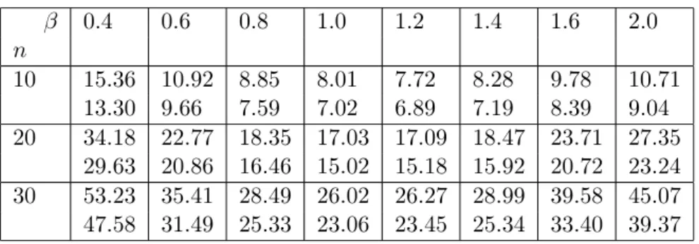
Since we could not find the expression for E(Q∗) under H1, we observed the direction of the test statistics by simulating its values for differentnand β and under different censoring proportionp(=r/n), 0< p <1. They are presented in Table 1.
Table 1: E(Q∗) for different values of β.
β 0.4 0.6 0.8 1.0 1.2 1.4 1.6 2.0
n
10 15.36 10.92 8.85 8.01 7.72 8.28 9.78 10.71 13.30 9.66 7.59 7.02 6.89 7.19 8.39 9.04 20 34.18 22.77 18.35 17.03 17.09 18.47 23.71 27.35
29.63 20.86 16.46 15.02 15.18 15.92 20.72 23.24 30 53.23 35.41 28.49 26.02 26.27 28.99 39.58 45.07 47.58 31.49 25.33 23.06 23.45 25.34 33.40 39.37 (The first value corresponds to 10% censoring and second value corresponds to 20% censoring).
The table shows that EH1(Q
∗)> E
H0(Q
∗) for 0< β <1 and for all n. For β >1, EH1(Q
∗) decreases below E
H0(Q
∗) for some range of β and then increases for β > 1.4. Thus the test procedure is to rejectH0 for large values of Q∗ in the above ranges.
3
Simulation study
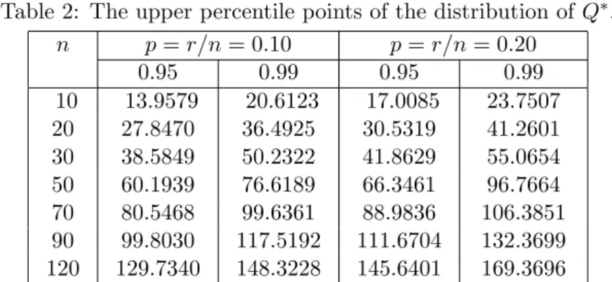
We obtain the upper tail percentile points of the distribution ofQby Monte Carlo method by generating 5000 random samples of different
sizes nfrom weibull distribution with θ =β = 1 and then construct type-2 with replacement censored samples under different censoring proportions. The results are given in Table 2.
Table 2: The upper percentile points of the distribution ofQ∗.
n p=r/n= 0.10 p=r/n= 0.20
0.95 0.99 0.95 0.99
10 13.9579 20.6123 17.0085 23.7507 20 27.8470 36.4925 30.5319 41.2601 30 38.5849 50.2322 41.8629 55.0654 50 60.1939 76.6189 66.3461 96.7664 70 80.5468 99.6361 88.9836 106.3851 90 99.8030 117.5192 111.6704 132.3699 120 129.7340 148.3228 145.6401 169.3696
We also compute the power of the test for different values of β
andn. The proposed test is compared with the test proposed by Bain and Engelhardt (1986), say BE test and is given as follows: A sizeα
test for testing H0 :β ≤ β0 against H1 :β ≥β0, the test reject H0 if cr(β0/βˆ)1+β
2
< χ2α(c(r−1)), where c = 2/[(1 +p2)2pc22]; p = r/n,
c22 is the asymptotic variance of ( ˆβ/β) and ˆβ is the MLE ofβ. The values of c22 is well tabulated (see Bain and Engelhardt, 1986) for different values ofn and p. Table 3 present the values of the powers of Q∗ and BE test correspond to β > 1 for 5% level of significance under different censoring schemes.
Table 3: Power of the test for IFR alternatives
n β = 1.4 β = 1.6 β = 1.8 β = 2.0
Q∗ BE Q∗ BE Q∗ BE Q∗ BE 10 .063 .062 .108 .107 .149 .144 .185 .184
.058 .055 .095 .101 .139 .137 .149 .144 20 .079 .073 .138 .133 .200 .198 .295 .290 .076 .072 .115 .114 .179 .172 .272 .271 30 .111 .115 .206 .210 .339 .336 .482 .479 .095 .111 .163 .155 .289 .286 .404 .402 50 .159 .165 .295 .288 .509 .502 .678 .677 .136 .143 .256 .251 .460 .455 .617 .615 120 .250 .259 .561 .558 .815 .813 .963 .956 .226 .230 516 .512 .779 .791 .949 .935 (The first value corresponds to 10% censoring and second value corresponds to 20% censoring).
From the above table it is seen that as the values of n and β
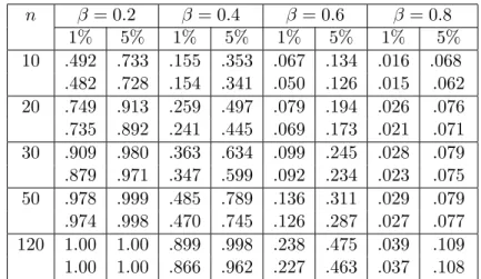
increases the power of the proposed test fairs better than the BE test. Table 4 presents the powers correspond toβ <1 forQ∗ test for both 1% and 5% level of significance.
Table 4: Power of the test for DFR alternatives
n β= 0.2 β= 0.4 β= 0.6 β = 0.8
1% 5% 1% 5% 1% 5% 1% 5%
10 .492 .733 .155 .353 .067 .134 .016 .068 .482 .728 .154 .341 .050 .126 .015 .062 20 .749 .913 .259 .497 .079 .194 .026 .076 .735 .892 .241 .445 .069 .173 .021 .071 30 .909 .980 .363 .634 .099 .245 .028 .079 .879 .971 .347 .599 .092 .234 .023 .075 50 .978 .999 .485 .789 .136 .311 .029 .079 .974 .998 .470 .745 .126 .287 .027 .077 120 1.00 1.00 .899 .998 .238 .475 .039 .109 1.00 1.00 .866 .962 .227 .463 .037 .108 (The first value corresponds to 10% censoring and second value corresponds to 20% censoring).
Thus from the above tables it is observed that the proposed test performs well for identifying both IFR and DFR alternatives under with replacement censored samples.
4
Example
We consider the data recorded based on a life test for a new insulating material. 25 specimens were tested simultaneously and the test was run until 15 of the specimens failed (for more details, see example 7.13 of Meeker and Escobar, 1998). Assuming that the data were recorded under with replacement scheme, we obtain the percentile points cor-respond to n = 25 and r = 15 as 62.83 and 88.14 respectively for upper 5% and 1% percentile points. Under the null hypothesis, the computed value of Q∗ is 112.78, which is larger than the percentile points corresponds to 1% and hence the test is rejected. The p-value correspond to this test is 0.004. The power corresponds to the specific alternatives say, H1 :β = 1.8 correspond to 1% and 5% are 0.11 and 0.18 respectively. Similarly, forH1 :β = 0.5, the powers are obtained as 0.24 and 0.35 respectively for 1% and 5% cutt-off points.
Acknowledgements
The author thanks the Editor for their comments. The author also acknowledges the University Grants Commission, New Delhi for sanc-tioning the research project no. F:6-7/2001 (SR-1).
References
Bain, L. J. and Engelhardt, M. (1986), Approximate distributional results based on the Maximum likelihood estimators for the weibull distribution. J. Quality Technology,18, 174-181. Bain, L. J. and Engelhardt, M. (1991), Statistical Analysis of
Re-liability and Life-testing Models. New York: Marcel Dekker Inc.
Graybill, F. A. (1969), Introduction to Matrices With Application in Statistics. Belmont, California: Wordsworth Publishing com-pany Inc.
Lawless, J. F. (1982), Statistical Models and Methods for Lifetime Data. New York: John Wiley & Sons.
Muralidharan, K. and Shanubhogue, A. (2004), A conditional test for exponentiality against weibull DFR alternatives based on censored samples. JIRSS,3(1), 69-81.
Reiss, R. D. (1989), Approximate Distribution of Order Statistics. New York: Springer-Verlag.
Thoman, D. R., Bain, L. J., and Antly, C. E. (1969), Inferences on the parameters of the weibull distribution. Technometrics.,11, 445-460.