Simultaneous reduction of emissions (CO
2and CO) and optimization
of production routing problem in a closed-loop supply chain
Yasser Emamian
1, Isa Nakhai Kamalabadi
1, Alireza Eydi
11 Department of Industrial Engineering, University of Kurdistan, Sanandaj, Iran [email protected], [email protected], [email protected]
Abstract
Environmental pollution and emissions, along with the increasing production and distribution of goods, have placed the future of humanity at stake. Today, measures such as the extensive reduction in emissions, especially of CO2 and CO, have been emphasized by most researchers as a solution to the problem of environmental protection. This paper sought to explore production routing problem in closed-loop supply chains in order to find a solution to reduce CO2 and CO emissions using the robust optimization technique in the process of product distribution. The uncertainty in some parameters, such as real-world demand, along with heterogeneous goals, compelled us to develop a fuzzy robust multi-objective model. Given the high complexity of the problem, metaheuristic methods are proposed for solving the model. To this end, the bee optimization method is developed. Some typical problems are solved to evaluate the solutions. In addition, in order to prove the algorithm’s efficiency, the results are compared with those of the genetic algorithm in terms of quality, dispersion, uniformity, and runtime. The dispersion index values showed that the bee colony algorithm produces more workable solutions for the exploration and extraction of the feasible region. The uniformity index values and the runtime results also indicate that the genetic algorithm provides shorter runtimes and searches the solution space in a more uniform manner, as compared with the bee colony algorithm.
Keywords:
Emissions, production routing, closed-loop supply chain, robust optimization1- Introduction
Environmental pollution caused by emissions, especially of CO2 and CO, is one of the major problems whose elimination requires the adoption of appropriate strategies. In December 2015, the United Nations Climate Change Conference was held in Paris. 195 countries from around the world attended the Conference. Based on the statistics released in the Conference, Iran ranks seventh in the production of greenhouse gases (GHGs). According to the Paris Convention, Iran has undertaken to reduce the pollution caused by greenhouse gases by 4% unconditionally and up to 12% conditionally (subject to international aids) in a 20-year period, starting from 2020. The transportation sector, as one of the key components of the supply chain, accounts for a large portion of this pollution. Therefore, exploring the production routing problem can significantly help us reduce CO2 and CO emissions by motor vehicles.
*Corresponding author
ISSN: 1735-8272, Copyright c 2018 JISE. All rights reserved
Journal of Industrial and Systems Engineering
Vol. 11, No.2, pp. 114-133
Spring (April) 2018
A supply chain consists of a sequence of activities involved in the production, lot sizing, distribution, and backflow of goods. Each activity is planned and optimized based on its associated predicted decisions. Transportation is of great importance in economic, manufacturing, and service systems and accounts for a sizeable part of the GDP of each country. Therefore, many researchers have attempted to find ways to improve routes, remove unnecessary trips, and propose alternative shortcuts (Taghavifard et al, 2009). In routing and transportation problems, different objectives such as cost, risk, distance, and response-time minimization or quality, customer satisfaction, profit, and accountability maximization have been taken into account. Cost minimization or at most two of the aforementioned objectives are usually selected as the model’s goal by most researchers (Tavakkoli-Moghaddam et al, 2007).
In an attempt to develop new problems, some researchers have combined the Vehicle Routing Problem (VRP) with other problems. For example, some have proposed the Production Routing Problem (PRP). According to PRP, products are routed between different levels of the supply chain including supplier, manufacturer, distributor, and customer. Adulyasak et al. (2015) conducted an in-depth review study on PRP and concluded that most researchers have proposed heuristic and metaheuristic methods for solving this problem, while the use of exact algorithms and robust optimization techniques has been less taken into account. Adulyasak et al. (2014) developed a mathematical model of mixed integer for PRP in the supply chain which is a combination of problems for lot sizing and inventory-routing. Sun & Wang (2015) proposed an approach to the robust optimization technique for the routing problem while taking the uncertainties into consideration.
At the same time, in a transportation system, distributors, who are seeking to maximize their profit, are faced with multiple problems such as traffic congestion, air pollution, loss of time in daily trips, increased fuel consumption, and vehicle depreciation in the process of products distribution and cash earning. This has encouraged researchers to focus on objectives aimed at reducing environmentally polluting emissions, fuel consumption, traffic congestion, etc. For example, considering the conditions of simultaneous product pickup and delivery and the existing uncertainties, Tajik et al. (2014) proposed a robust optimization approach with a limited time window to the routing problem aimed at reducing pollution caused by motor vehicles.
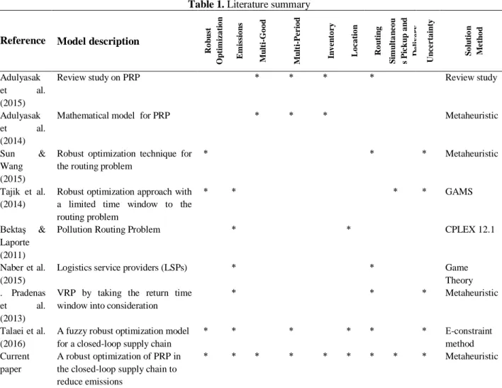
In terms of CO2 reduction, Bektaş & Laporte (2011) explored PRP as a developed version of VRP. Considering the time window, they proposed a mathematical model for minimizing trip time and emissions. In a study on the allocation of CO2 reduction to customers in distribution routing, Naber et al. (2015) explained the misunderstanding of logistics service providers (LSPs), both individuals and organizations, of the subject and modeled the problem using the cooperative game theory, while taking into consideration the amount of CO2 emissions produced in the entire transportation process. Pradenas et al. (2013) solved VRP by taking the return time window into consideration. Their attempt was aimed at reducing trip time and fuel consumption, and ultimately the emission of greenhouse gases. In addition, Talaei et al. (2016) proposed a fuzzy robust optimization model for a closed-loop supply chain, taking into consideration the relevant polluting emissions. First, they converted the fuzzy model into a deterministic model using the Jiménez ranking method, and consequently developed a robust optimization model.Table 1 briefly compares previous studies and shows the framework in this one.
Table 1. Literature summary S o lu ti o n M e th o d U n c e r ta in ty S im u lta n e o u s P ic k u p a n d D e li v e r y R o u ti n g Lo c a ti o n In v e n to r y M u lt i-P e r io d M u lt i-G o o d Em is si o n s R o b u st O p ti m iz a ti o n Model description Reference Review study * * * * Review study on PRP
Adulyasak
et al.
(2015)
Metaheuristic *
* * Mathematical model for PRP
Adulyasak
et al.
(2014)
Metaheuristic *
* *
Robust optimization technique for the routing problem
Sun &
Wang (2015) GAMS * * * * Robust optimization approach with a limited time window to the routing problem
Tajik et al. (2014)
CPLEX 12.1 *
* Pollution Routing Problem
Bektaş & Laporte (2011) Game Theory * * Logistics service providers (LSPs)
Naber et al. (2015)
Metaheuristic *
* *
VRP by taking the return time window into consideration . Pradenas
et al.
(2013) Ε-constraint method * * * * * * A fuzzy robust optimization model for a closed-loop supply chain Talaei et al.
(2016) Metaheuristic * * * * * * * * * A robust optimization of PRP in the closed-loop supply chain to reduce emissions
Current paper
In this study, a mathematical model is proposed for PRP in a closed-loop supply chain in order to reduce CO2 and CO emissions, while aiming at robust optimization and minimization of carbon emissions. Accordingly, a mathematical model is first developed. This model is based on research studies by Adulyasak et al. (2014) and Tajik et al. (2014) and is widely used in different industries such as the petrochemical industry. Next, metaheuristic algorithms are used for problem-solving.
In the model proposed by Adulyasak et al. (2014), PRP is modeled in the context of a multi-node network. In addition, Tajik et al. (2014) merely modeled a Green Vehicle Routing Problem (G-VRP) by focusing on simultaneous pickup and delivery. However, the model proposed in the present study includes the unified modeling of a closed-loop supply chain focused on different levels of forward and reverse logistics and addresses PRP with regard to conditions of simultaneous pickup and delivery. Simultaneous pickup and delivery means that, in the last layer of direct supply chain logistics, vehicles that deliver goods to customers will also receive their returned goods.
Since this study dealt with routing solutions aimed at reducing CO2 and CO emissions, carbon emissions minimization is taken as one of the models expected objectives. At the same time, as there is no certainty regarding the supply chain parameters, especially the real-world demand, one of the most important decisions taken in the supply chain concerns the chain’s effectiveness and efficiency as combined with uncertain parameters and variables. Uncertainty in the supply chain results in the non-optimal decisions taken based on certainty assumptions. Hence, achieving a robust optimization based on fuzzy demand is taken as one of the proposed model’s objectives.
2- Mathematical modeling
The model dealt with location distributor facilities and reverse logistics facilities (collection and recovery, disposal, and recycling). In addition, vehicle routing with limited weight and volume capacity is included in the model. Due to the uncertainty of real-world problems, the robust optimization technique is used to achieve robustness in the face of uncertainty. Figure 1 depicts the conceptual model of the problem.As evident from figure 1, goods are manufactured in manufacturing centers and are then sent to distribution centers. In addition, surplus goods in manufacturing centers are sent to warehouses. Therefore, distribution centers receive the goods they require from manufacturing centers or their warehouses in each period. Goods are then transported from distribution centers to customers and distributed among them. The goods returned by customers for various reasons are received and sent to collection and recovery centers. If possible, the retuned goods will be reclaimed and processed at these centers and sent back to distribution centers to be delivered to customers. If the goods need to be recycled, they will be sent to recycling centers to re-enter the production cycle. If goods cannot be processed, they will be sent to disposal centers. Therefore, the problem includes routing, manufacturing, distribution, inventory, and location, all, aimed at minimizing carbon emissions in a multi-level, multi-good, and multi-period green supply chain.
Fig 1. Remanufacturing and collection centers for the conceptual closed loop supply chain.
Modeling assumptions
The mathematical modeling is based on the following assumptions:
Goods are considered as packages containing a certain amount of a solid produced good.
Goods are produced in manufacturing centers and sent to distribution centers or warehouses.
Distribution centers receive the required goods from manufacturing centers or warehouses.
There number of available vehicles (trucks) is limited and specified. In addition, each vehicle can carry a limited volume of goods.
A vehicle may carry shipments for several distributors. Hence, after delivering the goods to the distributor j1, it may leave for other distributors, for example, j2. Therefore, the vehicle also travels between distributors.
A vehicle may carry shipments for several customers. Hence, following the delivery of the goods to customer l1, it may leave for other customers, for example, l2. Therefore, the vehicle also travels between customer centers.
The number of potential points associated with distribution centers is predetermined. These centers have a limited capacity.
The number of customer (demand) points is predetermined. All these points must be met by vehicles. Customer demand is uncertain and determined as a triangular fuzzy number.
Delivery and payment are simultaneous.
Fuel consumption per unit of distance is determined based on the vehicle speed and cargo weight.
The distance between centers and fuel price per liter are predetermined.
The speed is considered varying for each vehicle.
The construction cost is determined as a triangular fuzzy number.
Model indices
𝐼 Set of fixed points for manufacturing centers; i ϵ I
𝐽 Set of potential points for distribution centers; j ϵ J
𝐾 Set of vehicles; k ϵ K
𝐿 Set of fixed points for customers; l, l1, l2 ϵ L
𝑀 Set of potential points for collection and recovery centers; m ϵ M
𝑁 Set of potential points for disposal centers; n ϵ N
𝑃 Set of potential pints for recycling centers; p ϵ P
𝑆 Set of products; s ϵ S
𝑇 Set of time periods; t ϵ T
𝑁𝐽 Set of distribution center nodes
𝑁𝐿 Set of demand points
Model parameters
𝑐𝑎𝑗 Capacity of distribution center at point j
𝑝𝑐 Mean price of each unit of emission
𝑝𝑓 Fuel price per unit of volume
𝑣𝑓 Volume of fuel consumed per unit of distance and unit of weight; speed and distance
𝑣𝑘 Speed of vehicle k
𝑣𝑜𝑙𝑠 Volume of product s
𝑤𝑐 Weight of emissions per a liter of consumed fuel
𝑤𝑘 Weight of vehicle k
𝑤𝑠 Weight of product s
𝛼𝑘 Coefficient of speed variation in vehicle k per unit of excessive weight
𝐿𝑖 Distance between manufacturing center i and its own warehouse
𝐿𝑖𝑗 Distance between manufacturing center i and distribution center j
𝐿𝑗𝑙 Distance between the distribution center j and the customer zone l
𝐿𝑙𝑚 Distance between demand point l and collection and recovery center m
𝐿𝑚𝑖 Distance between collection and recovery center m and manufacturing center i
𝐿𝑚𝑗 Distance between collection and recovery center m and distribution center j
𝐿𝑚𝑛 Distance between collection and recovery center m and disposal center n
𝐿𝑚𝑝 Distance between collection and recovery center m and recycling center p
𝐿𝑝𝑖 Distance between recycling center p and manufacturing center i
𝐿𝑙1𝑙2 Distance between demand point l1 and demand point l2
𝐿𝑄𝑖𝑗 Distance between the warehouse of manufacturing center i and distribution center j
𝑄𝑊𝑘 Weight capacity of vehicle k
𝑓̃𝑗 Fuzzy cost of construction of a distribution center at point j
𝑓̃𝑚 Fuzzy cost of construction of a collection and recovery center at point m
𝑓̃𝑛 Fuzzy cost of construction of a disposal center at point n
𝑓̃𝑝 Fuzzy cost of construction of a recycling center at point p
𝑑̃𝑙𝑠𝑡 Fuzzy demand for product s from demand point l in period t (fuzzy demand for delivery to demand
point)
𝑟̃𝑙𝑠𝑡 Fuzzy value of the return of product s from demand point l in period t (fuzzy value of customer payment)
Variables
𝑞𝑙𝑠𝑡 Unmet demand of customer l for good s in period t
𝑤𝑗𝑗𝑘𝑡𝑠 Amount of good s transported by vehicle k in period t before meeting distribution center j
𝑤𝑙𝑙𝑘𝑡𝑠 Amount of good s delivered by vehicle k in period t before meeting demand point l
𝑥𝑖𝑘𝑡𝑠 Amount of good s transported by vehicle k from manufacturing center i to its own warehouse in
period t
𝑥𝑖𝑗𝑘𝑡𝑠 Amount of good s transported by vehicle k from manufacturing center i to all distribution centers in period t initially meeting distribution center j
𝑥𝑗𝑙𝑘𝑡𝑠 Amount of good s transported by vehicle k from distribution center j to the demand points in period
t and initially meeting customer l
𝑥𝑙𝑚𝑘𝑡𝑠 Amount of good s received from demand point l by vehicle k in period t to be sent to collection and
recovery center m, at the same time the replacement product is delivered to the same customer
𝑥𝑚𝑛𝑘𝑡𝑠 Amount of good s transported by vehicle k from collection and recovery center m to disposal center
n in period t
𝑥𝑚𝑝𝑘𝑡𝑠 Amount of good s transported by vehicle k from collection and recovery center m to manufacturing
center i in period t
𝑥𝑚𝑖𝑘𝑡𝑠 Amount of good s transported by vehicle k from collection and recovery center m to manufacturing
center i in period t
𝑥𝑚𝑗𝑘𝑡𝑠 Amount of good s transported by vehicle k from collection and recovery center m to distribution center j in period t
𝑥𝑝𝑖𝑘𝑡𝑠 Amount of good s transported by vehicle k from recycling center p to manufacturing center i in period t
𝑥𝑝𝑖𝑡𝑠 Amount of good s produced by manufacturing center i in period t
𝑥𝑖𝑖𝑗𝑘𝑡𝑠 Amount of good s transported by vehicle k from the warehouse of manufacturing center i to all
distribution centers in period t and initially meeting distribution center j
𝑥𝑤𝑖𝑗𝑘𝑡𝑠 Amount of good s transported by vehicle k from manufacturing center i to all distribution centers in period t initially meeting distribution center j and being delivered to distribution center j
𝑥𝑤𝑗𝑙𝑘𝑡𝑠 Amount of good s transported by vehicle k from distribution center j to demand points in period t
initially meeting demand point l and being delivered to demand point l
𝑥𝑖𝑤𝑖𝑗𝑘𝑡𝑠 Amount of good s transported by vehicle k from the warehouse of manufacturing center i to all distribution centers in period t initially meeting distribution center j and being delivered to distribution center j
𝑥𝑤𝑗1𝑗2𝑘𝑡𝑠 Amount of good s transported by vehicle k from distribution center j1 to distribution center j2 in
period t being delivered to distribution center j2
𝑥𝑤𝑙1𝑙2𝑘𝑡𝑠 Amount of good s transported by vehicle k from demand point l1 to demand point l2 in period t and
being delivered to demand point l2
𝑦𝑖𝑘𝑡 If vehicle k leaves manufacturing center i for its own warehouse in period t, it will be equal to 1, and
otherwise to 0
𝑦𝑖𝑗𝑘𝑡 If vehicle k leaves manufacturing center i for distribution center j in period t, it will be equal to 1, and otherwise to 0
𝑦𝑗𝑙𝑘𝑡 If vehicle k leaves distribution center j for demand point (customer) l in period t, it will be equal to
1, and otherwise to 0
𝑦𝑙𝑚𝑘𝑡 If vehicle k leaves demand point l for collection and recovery center m in period t, it will be equal to 1, and otherwise to 0
𝑦𝑚𝑖𝑘𝑡 If vehicle k leaves collection and recovery center m for manufacturing center i in period t, it will be equal to 1, and otherwise 0
𝑦𝑚𝑗𝑘𝑡 If vehicle k leaves collection and recovery center m for distribution center j in period t, it will be equal to 1, and otherwise to 0
𝑦𝑚𝑛𝑘𝑡 If vehicle k leaves collection and recovery center m for disposal center n in period t, it will be equal to 1, and otherwise to 0
𝑦𝑚𝑝𝑘𝑡 If vehicle k leaves collection and recovery center m for recycling center p in period t, it will be equal to 1, and otherwise to 0
𝑦𝑝𝑖𝑘𝑡 If vehicle k leaves recycling center p for manufacturing center i in period t, it will be equal to 1, and otherwise to 0
𝑦𝑖𝑖𝑗𝑘𝑡 If vehicle k leaves the warehouse of manufacturing center i for distribution center j in period t, it will be equal to 1, and otherwise to 0
𝑦𝑗1𝑗2𝑘𝑡 If vehicle k leaves distribution center j1 for distribution center j2 in period t, it will be equal to 1,
and otherwise to 0
𝑦𝑙1𝑙2𝑘𝑡 If vehicle k leaves demand point l1 for demand point l2 in period t, it will be equal to 1, and
otherwise to 0
𝑧𝑗 If distribution center is established at point j, it will be equal to 1, and otherwise to 0
𝑧𝑚 If collection center is established at point m, it will be equal to 1, and otherwise to 0
𝑧𝑛 If disposal center is established at point n, it will be equal to 1, and otherwise to 0
𝑧𝑝 If recycling center is established at point p, it will be equal to 1, and otherwise to 0
2-1- Model
(1)
min z1 = ∑ 𝑓̃𝑗𝑧𝑗
𝐽
𝑗=1
+ ∑ 𝑓̃𝑚𝑧𝑚
𝑀
𝑚=1
+ ∑ 𝑓̃𝑝𝑧𝑝
𝑃
𝑝=1
+ ∑ 𝑓̃𝑛𝑧𝑛
𝑁
𝑛=1
+(∑(𝑣𝑓∗ 𝛼𝑘∗ 𝑣𝑘)
𝐾
𝑘=1
∗ ( ∑(∑(∑ (𝑥𝑖𝑘𝑡𝑠∗ 𝐿𝑖+ ∑(𝑥𝑖𝑖𝑗𝑘𝑡𝑠 ∗ 𝐿𝑄𝑖𝑗+ 𝑥𝑖𝑗𝑘𝑡𝑠 ∗ 𝐿𝑖𝑗)
𝐽 𝑗=1 ) 𝐼 𝑖=1 𝑇 𝑡=1
∗ 𝑤𝑠)
𝑆
𝑠=1
+ ∑(𝑤𝑗𝑗𝑘𝑡𝑠+ ∑ 𝑥𝑗𝑙𝑘𝑡𝑠 ∗ 𝐿𝑗𝑙
𝐿
𝑙=1
) ∗ 𝑤𝑠
𝐽
𝑗=1
+ ∑((𝑤𝑙𝑘𝑡𝑠+ ∑ 𝑥𝑤𝑗𝑙𝑘𝑡𝑠) +
𝐽
𝑗=1
∑ (𝑥𝑤𝑙1𝑙𝑘𝑡𝑠 ∗ 𝐿
𝑙1𝑙) 𝐿 𝑙1=1 ) 𝐿 𝑙=1
× 𝑤𝑠
+ ∑ (∑ 𝑥𝑙𝑚𝑘𝑡𝑠 ∗ 𝐿𝑙𝑚
𝐿
𝑙=1
+ ∑ 𝑥𝑚𝑖𝑘𝑡𝑠
𝐼
𝑖=1 𝑀
𝑚=1
∗ 𝐿𝑚𝑖+ ∑ 𝑥𝑚𝑗𝑘𝑡𝑠 ∗ 𝐿𝑚𝑗
𝐽
𝑗=1
+ ∑ 𝑥𝑚𝑛𝑘𝑡𝑠
𝑁
𝑛=1
∗ 𝐿𝑚𝑛
+ ∑ 𝑥𝑚𝑝𝑘𝑡𝑠 ∗ 𝐿𝑚𝑝)
𝑃
𝑝=1
∗ 𝑤𝑠) + ∑ ∑ 𝑥𝑝𝑖𝑘𝑡𝑠 ∗ 𝐿𝑝𝑖∗ 𝑤𝑠
𝐼
𝑖=1 𝑃
𝑝=1
+ 𝑤𝑘)) ∗ (𝑝𝑓+ 𝑤𝑐∗ 𝑝𝑐) )
(2)
min 𝑧2 = ∑ ∑ ∑𝑞𝑙𝑠
𝑡
𝑑̃𝑙𝑠𝑡
𝑆 𝑠=1 𝐿 𝑙=1 𝑇 𝑡=1 Subject to. (3)
∑ 𝑦𝑖𝑘𝑡
𝑘
= ∑ ∑ 𝑦𝑖𝑖𝑗𝑘𝑡
𝑗 𝑘
∀𝑖, 𝑡
(4)
∑(∑(𝑦𝑖𝑗𝑘𝑡
𝑖 𝑘
+ 𝑦𝑖𝑖𝑗𝑘𝑡 ) + ∑ 𝑦𝑚𝑗𝑘𝑡
𝑚
) = ∑(∑ 𝑦𝑗𝑙𝑘𝑡
𝑙 𝑘
+ ∑ 𝑦𝑗𝑗1𝑘𝑡
𝑗1
(5)
∑ ∑ 𝑦𝑗𝑙𝑘𝑡
𝑗 𝑘
= ∑(∑ 𝑦𝑙𝑚𝑘𝑡
𝑚 𝑘
+ ∑ 𝑦𝑙𝑙1𝑘𝑡
𝑙1
) ∀𝑙, 𝑡
(6)
∑ ∑ 𝑦𝑙𝑚𝑘𝑡
𝑙 𝑘
= ∑(∑ 𝑦𝑚𝑝𝑘𝑡
𝑝
+ ∑ 𝑦𝑚𝑛𝑘𝑡
𝑛 𝑘
+ ∑ 𝑦𝑚𝑗𝑘𝑡
𝑗
+ ∑ 𝑦𝑚𝑖𝑘𝑡
𝑖
) ∀𝑚, 𝑡
(7)
∑ ∑ 𝑦𝑚𝑝𝑘𝑡
𝑚 𝑘
= ∑ ∑ 𝑦𝑝𝑖𝑘𝑡
𝑖 𝑘
∀𝑝, 𝑡
(8)
∑ ∑ 𝑦𝑝𝑖𝑘𝑡
𝑝 𝑘
= ∑ ∑ 𝑦𝑖𝑘𝑡
𝑖 𝑘
+ ∑ ∑ 𝑦𝑖𝑗𝑘𝑡
𝑖 𝑘
∀𝑝, 𝑡
(9)
∑(∑ 𝑥𝑤𝑗𝑙𝑘𝑡𝑠
𝑗 𝑘
+ ∑ 𝑥𝑤𝑙1𝑙𝑘𝑡𝑠 )
𝑙1
+ 𝑞𝑙𝑠𝑡 = 𝑑̃𝑙𝑠𝑡 + 𝑟̃𝑙𝑠𝑡 ∀𝑙, 𝑡, 𝑠
(10)
𝑤𝑙𝑙1𝑘𝑡𝑠 − 𝑤𝑙
𝑙2𝑘
𝑡𝑠 ≥ ∑(𝑥𝑤
𝑗𝑙1𝑘𝑡𝑠 × 𝑦𝑗𝑙1𝑘𝑡 ) + 𝑗
∑(𝑥𝑤𝑙𝑙1𝑘𝑡𝑠 × 𝑦
𝑙𝑙1𝑘𝑡 ) 𝑙
+ 𝑥𝑙1𝑚𝑘𝑡𝑠 − 𝑀(1 − 𝑦
𝑙1𝑙2𝑘𝑡 ) ∀𝑙1, 𝑙2, 𝑙 ∈ 𝐿 , ∀𝑘, 𝑡, 𝑠
(11)
𝑥𝑝𝑖𝑡𝑠+ ∑ ∑ 𝑥𝑚𝑖𝑘𝑡𝑠
𝑚 𝑘
= ∑(𝑥𝑖𝑘𝑡𝑠+ ∑ 𝑥𝑖𝑗𝑘𝑡𝑠 ) ∀𝑖, 𝑡, 𝑠
𝑗 𝑘
(12)
∑(∑(𝑥𝑤𝑖𝑗𝑘𝑡𝑠
𝑖 𝑘
+ 𝑥𝑖𝑤𝑖𝑗𝑘𝑡𝑠) + ∑ 𝑥𝑚𝑗𝑘𝑡𝑠
𝑚
+ ∑ 𝑥𝑤𝑗1𝑗𝑘𝑡𝑠
𝑗1
) = ∑ ∑ 𝑥𝑗𝑙𝑘𝑡𝑠
𝑙 𝑘
∀𝑗, 𝑡, 𝑠
(13)
∑ ∑ 𝑥𝑙𝑚𝑘𝑡𝑠
𝑙 𝑘
= ∑(∑ 𝑥𝑚𝑝𝑘𝑡𝑠
𝑝
+ ∑ 𝑥𝑚𝑛𝑘𝑡𝑠
𝑛 𝑘
+ ∑ 𝑥𝑚𝑗𝑘𝑡𝑠
𝑗
+ ∑ 𝑥𝑚𝑖𝑘𝑡𝑠
𝑖
) ∀𝑚, 𝑡, 𝑠
(14)
𝑤𝑗𝑗1𝑘𝑡𝑠 − 𝑤𝑗𝑗2𝑘𝑡𝑠 ≥ ∑(𝑥𝑤𝑖𝑗1𝑘𝑡𝑠 × 𝑦𝑖𝑗1𝑘𝑡 ) +
𝑖
∑(𝑥𝑤𝑗𝑗1𝑘𝑡𝑠 × 𝑦
𝑗𝑗1𝑘𝑡 ) 𝑗
− 𝑀(1 − 𝑦𝑗1𝑗2𝑘𝑡 ) ∀(𝑗1, 𝑗2) ∈ 𝐽 × 𝐽, ∀𝑘, 𝑡, 𝑠
(15)
∑ ∑ 𝑦𝑗1𝑗2𝑘𝑡
𝑗2∈𝑁 𝑗1∈𝑁
≤ |𝑁| − 1 ∀𝑁 ∈ 𝑁𝐽: |𝑁| ≥ 2 &∀𝑘, 𝑡
(16)
∑ ∑ 𝑦𝑙1𝑙2𝑘𝑡
𝑙2∈𝑁 𝑙1∈𝑁
≤ |𝑁| − 1 ∀𝑁 ∈ 𝑁𝐿: |𝑁| ≥ 2 &∀𝑘, 𝑡
(17)
∑ ∑(∑(𝑥𝑖𝑤𝑖𝑗𝑘𝑡𝑠 + 𝑥𝑤𝑖𝑗𝑘𝑡𝑠)
𝑖
+ ∑ 𝑥𝑤𝑗1𝑗𝑘𝑡𝑠
𝑗1 𝑘
𝑠
) ≤ 𝑐𝑎𝑗 ∀𝑗, 𝑡
(18)
∑((𝑤𝑙𝑙1𝑘𝑡𝑠 + ∑(𝑥𝑤𝑗𝑙1𝑘𝑡𝑠 × 𝑦𝑗𝑙1𝑘𝑡 ) +
𝑗
∑(𝑥𝑤𝑙𝑙1𝑘𝑡𝑠 × 𝑦𝑙𝑙1𝑘𝑡 )
𝑙
+ 𝑥𝑙1𝑘𝑡𝑠 )
𝑠
× 𝑤𝑠) ≤ 𝑄𝑊𝑘 ∀𝑙, 𝑘, 𝑡
(19)
∑((𝑤𝑙𝑙1𝑘𝑡𝑠 + ∑(𝑥𝑤𝑗𝑙1𝑘𝑡𝑠 × 𝑦𝑗𝑙1𝑘𝑡 ) +
𝑗
∑(𝑥𝑤𝑙𝑙1𝑘𝑡𝑠 × 𝑦𝑙𝑙1𝑘𝑡 )
𝑙
+ 𝑥𝑙1𝑘𝑡𝑠 )
𝑠
× 𝑣𝑜𝑙𝑠) ≤ 𝑄𝑉𝑘 ∀𝑙, 𝑘, 𝑡
(44)
𝑥𝑖𝑖𝑗𝑘𝑡𝑠 ≤ 𝑀 × 𝑦𝑖𝑖𝑗𝑘𝑡 ∀𝑖, 𝑗, 𝑘, 𝑡, 𝑠
(20)
∑(𝑥𝑖𝑘𝑡𝑠× 𝑤𝑠)
𝑠
≤ 𝑄𝑊𝑘 ∀𝑖, 𝑘, 𝑡
(45)
𝑥𝑤𝑖𝑗𝑘𝑡𝑠 ≤ 𝑀 × 𝑦𝑖𝑗𝑘𝑡 ∀𝑖, 𝑗, 𝑘, 𝑡, 𝑠
(21)
∑(𝑥𝑖𝑘𝑡𝑠× 𝑣𝑜𝑙𝑠)
𝑠
≤ 𝑄𝑉𝑘 ∀𝑖, 𝑘, 𝑡
(46)
𝑥𝑖𝑤𝑖𝑗𝑘𝑡𝑠 ≤ 𝑀 × 𝑦𝑖𝑖𝑗𝑘𝑡 ∀𝑖, 𝑗, 𝑘, 𝑡, 𝑠
(22)
∑(𝑥𝑖𝑖𝑗𝑘𝑡𝑠 × 𝑤𝑠)
𝑠
≤ 𝑄𝑊𝑘 ∀𝑖, 𝑗, 𝑘, 𝑡
(47) 𝑥𝑤𝑗1𝑗2𝑘𝑡𝑠 ≤ 𝑀 × 𝑦
𝑗1𝑗2𝑘𝑡 ∀𝑗1, 𝑗2, 𝑘, 𝑡, 𝑠 (23)
∑(𝑥𝑖𝑖𝑗𝑘𝑡𝑠 × 𝑣𝑜𝑙𝑠)
𝑠
≤ 𝑄𝑉𝑘 ∀𝑖, 𝑗, 𝑘, 𝑡
(48)
𝑥𝑗𝑙𝑘𝑡𝑠 ≤ 𝑀 × 𝑦𝑗𝑙𝑘𝑡 ∀𝑙, 𝑗, 𝑘, 𝑡, 𝑠
(24)
∑(𝑥𝑖𝑗𝑘𝑡𝑠 × 𝑤
𝑠) 𝑠
≤ 𝑄𝑊𝑘 ∀𝑖, 𝑗, 𝑘, 𝑡
(49)
𝑥𝑤𝑗𝑙𝑘𝑡𝑠 ≤ 𝑀 × 𝑦𝑗𝑙𝑘𝑡 ∀𝑙, 𝑗, 𝑘, 𝑡, 𝑠
(25)
∑(𝑥𝑖𝑗𝑘𝑡𝑠 × 𝑣𝑜𝑙
𝑠) 𝑠
≤ 𝑄𝑉𝑘 ∀𝑖, 𝑗, 𝑘, 𝑡
(50) 𝑥𝑤𝑙1𝑙2𝑘𝑡𝑠 ≤ 𝑀 × 𝑦𝑙1𝑙2𝑘𝑡 ∀𝑙1, 𝑙2, 𝑘, 𝑡, 𝑠
(26)
∑(𝑥𝑗𝑙𝑘𝑡𝑠 × 𝑤
𝑠) 𝑠
(51)
𝑥𝑙𝑚𝑘𝑡𝑠 ≤ 𝑀 × 𝑦𝑙𝑚𝑘𝑡 ∀𝑙, 𝑚, 𝑘, 𝑡, 𝑠
(27)
∑(𝑥𝑗𝑙𝑘𝑡𝑠 × 𝑣𝑜𝑙
𝑠) 𝑠
≤ 𝑄𝑉𝑘 ∀𝑗, 𝑙, 𝑘, 𝑡
(52)
𝑥𝑚𝑝𝑘𝑡𝑠 ≤ 𝑀 × 𝑦𝑚𝑝𝑘𝑡 ∀𝑝, 𝑚, 𝑘, 𝑡, 𝑠
(28)
∑(𝑥𝑚𝑝𝑘𝑡𝑠 × 𝑤𝑠)
𝑠
≤ 𝑄𝑊𝑘 ∀𝑚, 𝑝, 𝑘, 𝑡
(53)
𝑥𝑚𝑛𝑘𝑡𝑠 ≤ 𝑀 × 𝑦𝑚𝑛𝑘𝑡 ∀𝑛, 𝑚, 𝑘, 𝑡, 𝑠
(29)
∑(𝑥𝑚𝑝𝑘𝑡𝑠 × 𝑣𝑜𝑙
𝑠) 𝑠
≤ 𝑄𝑉𝑘 ∀𝑚, 𝑝, 𝑘, 𝑡
(54)
𝑥𝑚𝑖𝑘𝑡𝑠 ≤ 𝑀 × 𝑦𝑚𝑖𝑘𝑡 ∀𝑖, 𝑚, 𝑘, 𝑡, 𝑠
(30)
∑(𝑥𝑚𝑛𝑘𝑡𝑠 × 𝑤𝑠)
𝑠
≤ 𝑄𝑊𝑘 ∀𝑚, 𝑛, 𝑘, 𝑡
(55)
𝑥𝑚𝑗𝑘𝑡𝑠 ≤ 𝑀 × 𝑦𝑚𝑗𝑘𝑡 ∀𝑗, 𝑚, 𝑘, 𝑡, 𝑠
(31)
∑(𝑥𝑚𝑛𝑘𝑡𝑠 × 𝑣𝑜𝑙𝑠)
𝑠
≤ 𝑄𝑉𝑘 ∀𝑚, 𝑛, 𝑘, 𝑡
(56) 𝑦𝑗1𝑗2𝑘𝑡 ≤ 𝑀 × 𝑧
𝑗1× 𝑧𝑗2 ∀𝑗1, 𝑗2, 𝑘, 𝑡
(32)
∑(𝑥𝑚𝑖𝑘𝑡𝑠 × 𝑤
𝑠) 𝑠
≤ 𝑄𝑊𝑘 ∀𝑚, 𝑖, 𝑘, 𝑡
(57)
𝑦𝑗𝑙𝑘𝑡 ≤ 𝑀 × 𝑧𝑗 ∀𝑙, 𝑗, 𝑘, 𝑡
(33)
∑(𝑥𝑚𝑖𝑘𝑡𝑠 × 𝑣𝑜𝑙
𝑠) 𝑠
≤ 𝑄𝑉𝑘 ∀𝑚, 𝑖, 𝑘, 𝑡
(58)
𝑦𝑙𝑚𝑘𝑡 ≤ 𝑀 × 𝑧𝑚 ∀𝑙, 𝑚, 𝑘, 𝑡
(34)
∑(𝑥𝑚𝑗𝑘𝑡𝑠 × 𝑤𝑠)
𝑠
≤ 𝑄𝑊𝑘 ∀𝑚, 𝑗, 𝑘, 𝑡
(59)
𝑦𝑚𝑝𝑘𝑡 ≤ 𝑀 × 𝑧𝑚× 𝑧𝑝 ∀𝑝, 𝑚, 𝑘, 𝑡
(35)
∑(𝑥𝑚𝑗𝑘𝑡𝑠 × 𝑣𝑜𝑙𝑠)
𝑠
≤ 𝑄𝑉𝑘 ∀𝑚, 𝑗, 𝑘, 𝑡
(60)
𝑦𝑚𝑛𝑘𝑡 ≤ 𝑀 × 𝑧
𝑚× 𝑧𝑛 ∀𝑛, 𝑚, 𝑘, 𝑡
(36)
∑ ∑(𝑥𝑙𝑚𝑘𝑡𝑠 × 𝑤
𝑠) 𝑠
𝑙
≤ 𝑄𝑊𝑘 ∀𝑚, 𝑘, 𝑡
(61)
𝑦𝑚𝑖𝑘𝑡 ≤ 𝑀 × 𝑧𝑚 ∀𝑖, 𝑚, 𝑘, 𝑡
(37)
∑ ∑(𝑥𝑙𝑚𝑘𝑡𝑠 × 𝑣𝑜𝑙
𝑠) 𝑠
𝑙
≤ 𝑄𝑉𝑘 ∀𝑚, 𝑘, 𝑡
(62)
𝑦𝑚𝑗𝑘𝑡 ≤ 𝑀 × 𝑧𝑚 ∀𝑗, 𝑚, 𝑘, 𝑡
(38)
∑ ∑(𝑥𝑝𝑖𝑘𝑡𝑠 × 𝑤
𝑠) 𝑠
𝑙
≤ 𝑄𝑊𝑘 ∀𝑚, 𝑘, 𝑡
(63)
𝑦𝑖𝑗𝑘𝑡 ≤ 𝑀 × 𝑧𝑗 ∀𝑖, 𝑗, 𝑘, 𝑡
(39)
∑ ∑(𝑥𝑝𝑖𝑘𝑡𝑠 × 𝑣𝑜𝑙
𝑠) 𝑠
𝑙
≤ 𝑄𝑉𝑘 ∀𝑚, 𝑘, 𝑡
(64)
𝑦𝑖𝑖𝑗𝑘𝑡 ≤ 𝑀 × 𝑧𝑗 ∀𝑖, 𝑗, 𝑘, 𝑡
(65)
∑ 𝑧𝑗≥ 1 ∀𝑗
𝑗 (40)
∑ ∑ 𝑦𝑗𝑙𝑘𝑡 ≥ 1 ∀𝑙, 𝑡
𝑘 𝑗
(66)
∑ 𝑧𝑚≥ 1 ∀𝑚
𝑚 (41)
∑ 𝑥𝑙𝑘𝑡𝑠
𝑘
= 𝑟̃𝑙𝑠𝑡 ∀𝑙, 𝑡, 𝑠
(67)
∑ 𝑧𝑝≥ 1 ∀𝑝
𝑝 (42)
𝑥𝑖𝑘𝑡𝑠≤ 𝑀 × 𝑦𝑖𝑘𝑡 ∀𝑖, 𝑘, 𝑡, 𝑠
(68)
∑ 𝑧𝑛≥ 1 ∀𝑛
𝑛 (43)
𝑥𝑖𝑗𝑘𝑡𝑠 ≤ 𝑀 × 𝑦𝑖𝑗𝑘𝑡 ∀𝑖, 𝑗, 𝑘, 𝑡, 𝑠
(69) 𝑧𝑗, 𝑧𝑝, 𝑧𝑚, 𝑧𝑛, 𝑦𝑖𝑘𝑡, 𝑦𝑖𝑗𝑘𝑡 , 𝑦𝑖𝑖𝑗𝑘𝑡 , 𝑦𝑗𝑙𝑘𝑡 , 𝑦𝑗1𝑗2𝑘𝑡 , 𝑦𝑙1𝑙2𝑘𝑡 , 𝑦𝑙𝑚𝑘𝑡 , 𝑦𝑚𝑛𝑘𝑡 , 𝑦𝑚𝑝𝑘𝑡 , 𝑦𝑚𝑖𝑘𝑡 , 𝑦𝑚𝑗𝑘𝑡 ∈ {0,1}
(70)
𝑥𝑝𝑖𝑡𝑠, 𝑥𝑖𝑗𝑘𝑡𝑠 , 𝑥𝑖𝑘𝑡𝑠, 𝑥𝑖𝑖𝑗𝑘𝑡𝑠 , 𝑥𝑤𝑖𝑗𝑘𝑡𝑠, 𝑥𝑖𝑤𝑖𝑗𝑘𝑡𝑠, 𝑤𝑗𝑗𝑘𝑡𝑠, 𝑥𝑤𝑗1𝑗2𝑘𝑡𝑠 , 𝑥𝑗𝑙𝑘𝑡𝑠, 𝑥𝑤𝑗𝑙𝑘𝑡𝑠, 𝑥𝑤𝑙1𝑙2𝑘𝑡𝑠 , 𝑤𝑙𝑙𝑘𝑡𝑠, 𝑥𝑙𝑘𝑡𝑠, 𝑥𝑡𝑠𝑚𝑘, 𝑥𝑚𝑛𝑘𝑡𝑠 , 𝑥𝑚𝑝𝑘𝑡𝑠 , 𝑥𝑚𝑖𝑘𝑡𝑠 , 𝑥𝑚𝑗𝑘𝑡𝑠 ,
𝐼𝑙𝑠𝑡, 𝑞
𝑙𝑠𝑡 ≥ 0
Equation (1) shows the first objective function. This function involves minimization of facilities’ construction costs, vehicle fuel costs, and environmental costs of emissions. Equation (2) represents the second objective function which involves the total ratio of unmet demands of customers to their total demand for all goods in all periods. Constraints (3) to (8) indicate that the vehicles entering manufacturing centers and their warehouses, distribution centers, demand points, collection and recovery centers, and recycling centers will surely leave these points. In addition, the vehicles entering disposal centers will re-enter the cycle and begin from manufacturing cre-enters. They go to the manufacturing cre-enters as needed. Constraint (9) represents the amount of unmet demands of customer l for good s in period t. Constraint (10) calculates the amount of the inventory of good s in the cargo of vehicle k in period t before meeting
demand points. Constraints (11), (12), and (13) guarantee the balance of goods flow in nodes. Constraint (14) calculates the amount of the inventory of good s in the cargo of vehicle k in period t before meeting distribution centers. Constraints (15) and (16) prevent sub-tours during the trip of vehicles between distribution centers and demand points, respectively. Constraint (17) shows that the capacity of distribution centers is limited in terms of the number of goods they can carry. Constraints (18) to (39) ensure that goods transported by vehicle k do not exceed its weight and cubic capacity. Constraint (40) ensures that all customers are met by at least one of the vehicles in all periods. Constraint (41) ensures that all returned goods from demand points are collected in the backflow. Constraints (42) to (55) ensure that a good is transported from one center to another by a vehicle when the vehicle takes a trip between these two points. Constraints (56) to (64) ensure that a vehicle travels between two centers only when they are already established. Constraints (65) to (68) ensure that at least one center is established for facilities associated with distribution, collection, disposal, and recycling activities. Constraints (69) and (70) are related to symbols and allowed values for the model’s decision variables.
2-2- Robust optimization planning model
As can be seen, the proposed model is a dual-objective one with fuzzy parameters. First, the fuzzy model is converted into a corresponding deterministic model using the Jiménez ranking method (Jiménez et al., 2007). Next, the robust optimization planning model is developed.
The final form of objective functions after defuzzification:
(71)
min z1 = ∑(𝑓𝑗 1+ 2𝑓
𝑗2+ 𝑓𝑗3
2 )𝑧𝑗
𝐽
𝑗=1
+ ∑ (𝑓𝑚 1+ 2𝑓
𝑚2+ 𝑓𝑚3
2 )𝑧𝑚
𝑀
𝑚=1
+ ∑(𝑓𝑝 1+ 2𝑓
𝑝2+ 𝑓𝑝3
2 )𝑧𝑝
𝑃
𝑝=1
+ ∑(𝑓𝑛 1+ 2𝑓
𝑛2+ 𝑓𝑛3
2 )𝑧𝑛 𝑁 𝑛=1 +(∑(𝑣𝑓 𝐾 𝑘=1 ∗ 𝛼𝑘∗ 𝑣𝑘) ∗ ( ∑(∑(∑ (𝑥𝑖𝑘𝑡𝑠∗ 𝐿𝑖+ ∑(𝑥𝑖𝑖𝑗𝑘𝑡𝑠 ∗ 𝐿𝑄𝑖𝑗+ 𝑥𝑖𝑗𝑘𝑡𝑠 ∗ 𝐿𝑖𝑗)
𝐽 𝑗=1 ) 𝐼 𝑖=1 𝑇 𝑡=1 ∗ 𝑤𝑠) 𝑆 𝑠=1 + ∑(𝑤𝑗𝑗𝑘𝑡𝑠+ ∑ 𝑥𝑗𝑙𝑘𝑡𝑠 ∗ 𝐿𝑗𝑙
𝐿
𝑙=1
) ∗ 𝑤𝑠 𝐽
𝑗=1
+ ∑((𝑤𝑙𝑘𝑡𝑠+ ∑ 𝑥𝑤𝑗𝑙𝑘𝑡𝑠) + 𝐽
𝑗=1
∑ (𝑥𝑤𝑙1𝑙𝑘𝑡𝑠 ∗ 𝐿𝑙1𝑙) 𝐿 𝑙1=1 ) 𝐿 𝑙=1 × 𝑤𝑠
+ ∑ (∑ 𝑥𝑙𝑚𝑘𝑡𝑠 ∗ 𝐿𝑙𝑚 𝐿
𝑙=1
+ ∑ 𝑥𝑚𝑖𝑘𝑡𝑠 𝐼
𝑖=1 𝑀
𝑚=1
∗ 𝐿𝑚𝑖+ ∑ 𝑥𝑚𝑗𝑘𝑡𝑠 ∗ 𝐿𝑚𝑗 𝐽
𝑗=1
+ ∑ 𝑥𝑚𝑛𝑘𝑡𝑠 𝑁
𝑛=1
∗ 𝐿𝑚𝑛+ ∑ 𝑥𝑚𝑝𝑘𝑡𝑠 ∗ 𝐿𝑚𝑝) 𝑃
𝑝=1
∗ 𝑤𝑠)
+ ∑ ∑ 𝑥𝑝𝑖𝑘𝑡𝑠 ∗ 𝐿𝑝𝑖∗ 𝑤𝑠 𝐼
𝑖=1 𝑃
𝑝=1
+ 𝑤𝑘)) ∗ (𝑝𝑓+ 𝑤𝑐∗ 𝑝𝑐) )
(72)
min 𝑧2 = ∑ ∑ ∑ 𝑞𝑙𝑠
𝑡
(𝑑𝑙𝑠𝑡1+ 2𝑑𝑙𝑠𝑡2+ 𝑑𝑙𝑠𝑡3
2 ) 𝑆 𝑠=1 𝐿 𝑙=1 𝑇 𝑡=1
Constraint (9) after defuzzification:
(73)
∑(∑ 𝑥𝑤𝑗𝑙𝑘𝑡𝑠
𝑗 𝑘
+ ∑ 𝑥𝑤𝑙1𝑙𝑘𝑡𝑠 )
𝑙1
+ 𝑞𝑙𝑠𝑡
= (1 − 𝛼)𝑑𝑙𝑠
𝑡1+ 𝑑 𝑙𝑠𝑡2
2 + 𝛼
𝑑𝑙𝑠𝑡2+ 𝑑
𝑙𝑠 𝑡3
2 + (1 − 𝛼)
𝑟𝑙𝑠𝑡1+ 𝑟
𝑙𝑠𝑡2
2 + 𝛼
𝑟𝑙𝑠𝑡2+ 𝑟
𝑙𝑠𝑡3
2 ∀𝑙, 𝑡, 𝑠
Constraint (41) after defuzzification:
(74)
∑ 𝑥𝑙𝑘𝑡𝑠
𝑘
= (1 − 𝛼)𝑟𝑙𝑠
𝑡1+ 𝑟 𝑙𝑠𝑡2
2 + 𝛼
𝑟𝑙𝑠𝑡2+ 𝑟𝑙𝑠𝑡3
2 ∀𝑙, 𝑡, 𝑠
For a robust modeling based on demand, the first objective function remained unchanged. Other changes, assuming the definition of E(z2) being equal to Constraint (75), are as follows:
(75)
𝐸(𝑧2) = ∑ ∑ ∑𝑞𝑙𝑠
𝑡
𝑑𝑙𝑠𝑡
𝑆 𝑠=1 𝐿 𝑙=1 𝑇 𝑡=1
(76)
min 𝑧2 = 𝐸(𝑧2) + 𝛾(𝑧𝑚𝑎𝑥− 𝐸(𝑧2)) + 𝜑1 [(1 − 𝛼)
𝑑𝑙𝑠1,1+ 𝑑𝑙𝑠1,2
2 + 𝛼
𝑑𝑙𝑠1,2+ 𝑑𝑙𝑠1,3
2 + (1 − 𝛼)
𝑟𝑙𝑠1,1+ 𝑟𝑙𝑠1,2
2
+ 𝛼𝑟𝑙𝑠
1,2+ 𝑟 𝑙𝑠
1,3
2 ]
+ 𝜑2 [(1 − 𝛼)𝑑𝑙𝑠
𝑡1+ 𝑑 𝑙𝑠𝑡2
2 + 𝛼
𝑑𝑙𝑠𝑡2+ 𝑑𝑙𝑠𝑡3
2 + (1 − 𝛼)
𝑟𝑙𝑠𝑡1+ 𝑟𝑙𝑠𝑡2
2 + 𝛼
𝑟𝑙𝑠𝑡2+ 𝑟𝑙𝑠𝑡3
2 ]
+ 𝜑3 [(1 − 𝛼)𝑟𝑙𝑠
𝑡1+ 𝑟 𝑙𝑠𝑡2
2 + 𝛼
𝑟𝑙𝑠𝑡2+ 𝑟
𝑙𝑠𝑡3
2 ]
Where all the above constraints exist and 𝑧𝑚𝑎𝑥 is calculated as follows:
𝑧𝑚𝑎𝑥 = ∑ ∑ ∑
𝑞𝑙𝑠𝑡
d𝑙𝑠𝑡3
𝑆
𝑠=1 𝐿
𝑙=1 𝑇
𝑡=1
(77)
In Equation (76), 𝛾 represents the weight or importance of relevant statements in the objective function as compared with other objective components. In addition, 𝜑𝑖 denotes the penalty of deviation from equations with fuzzy parameters.
3- Solution methodology
Most of the logistics network design models, including the problem discussed in this study, are among the hard problems. These problems can be reduced to the problem of location facilities with limited capacity, which falls into the category of Np-Complete problems (Tibben-Lembke & Rogers, 2002). Therefore, the problem of logistics network design, discussed in this study, belongs to the category of Np-Hard problems. Due to high time complexity, precise methods cannot be used for solving these problems on a large scale. Thus, in this study, the bee optimization algorithm, which is based on Pareto archive, is used for solving the problem. The results obtained through this algorithm are compared with the results of the well-known NSGA-II algorithm.
3-1- Bee colony algorithm
Bee colony algorithm is an emerging group algorithm based on the foraging behavior of honey bees (Pham et al., 2006). The following structure is applied for implementing the bee colony algorithm aimed at solving the proposed model.
3-1-1- Solution representation
In this study, solutions are represented as matrices. Each solution contains several matrices developed according to the model outputs. For example, for Zm, a row (one-dimensional) matrix is defined whose
entries are equal to m (the number of collection centers); for 𝑦𝑖𝑘𝑡 , a three-dimensional matrix with dimensions of l, k, and t is defined; and for 𝑥𝑖𝑗𝑘𝑡𝑠 , a five-dimensional matrix with dimensions i, j, k, t, and s
is defined. Similarly, a matrix is defined to test the outputs.
3-1-2- Development of initial solutions
In the present study, a random approach is used for development of initial solutions. To this end, matrices Zj, Zm, Zp, and Zn are randomly developed and the remaining solution matrices (the model
variables) are feasibly initialized while taking the model constraints into consideration. Suppose that the size of the population is equal to N. Each time a solution is developed as explained, it will be added to the population unless it is iterative. This continues until the number of solutions in the population reaches α ×
N, where α is a number greater than 1.
Development of solutions is stopped after α × N iteration. At the same time, the number of solutions in each algorithm iteration is equal to N. Therefore, out of α × N solutions available, N solutions should be selected as the sequence of initial development. In this study, the initial population of solutions is selected based on a rapid method to sort the non-dominant solutions as explained by Deb et al. (2002). In this method, the α × N solutions available are sorted and ranked. The number of each rank represents the
quality of solutions available in that rank. For instance, the quality of solutions in Rank 1 is higher than those in Rank 2. Then, a scale known as the crowding distance is calculated for solutions available in each rank. This scale indicates the dispersion of available solutions in each rank.
In the present study, an index named 𝐶𝑠 isdefined for the selection of initial solutions. This index is
calculated as follows (Tavakkoli-Moghaddam et al., 2011):
𝐶𝑠=
𝑟𝑎𝑛𝑘
𝑐𝑟𝑜𝑤𝑑𝑖𝑛𝑔_𝑑𝑖𝑠 (78)
This is calculated for each of the available solutions.
rank = number of the rank the available solutions belong to
crowding-dis = crowding distance of each solution commensurate with its rank
After calculating the above index for all solutions, the solutions are ascending sorted in terms of 𝐶𝑠 and
the N first solutions with lower 𝐶𝑠are selected as the initial algorithm solutions. The use of 𝐶𝑠 is premised
upon the logic that solutions of higher quality and dispersion should be selected as the initial population. Solutions developed using this procedure, are improved so far as possible. The improvement procedure is described in the following section.
3-1-3- Improvement procedure
In the proposed structure of the bee colony optimization algorithm, an improvement procedure is developed which can be applied to the solutions selected in the previous section. The solutions produced through this procedure are selected as the next iteration population of the algorithm. In this study, the improvement procedure is implemented based on the variable neighborhood search (VNS), which uses four neighborhood search structures (NSS). These structures are in the form of VNS (See Tavakkoli-Moghaddam et al., (2011) for additional information on these structures). Each of the solutions in the population is inserted into the VNS algorithm and one single solution is received as the output. Next, the improvement procedure is applied on the remaining solution matrices to feasibly modify and replace the input solution. In addition, the neighborhood search operators used in the VNS structure are as follows:
• The first neighborhood search operator: In this structure, one of the distribution centers is randomly selected and its location matrix is changed.
• The second neighborhood search operator: In this structure, one of the collection centers is randomly selected and its location matrix is changed.
• The third neighborhood search operator: In this structure, one of the recycling centers is randomly selected and its location matrix is changed.
• The fourth neighborhood search operator: In this structure, one of the disposal centers is randomly selected and its location matrix is changed.
For changing the location matrix in the above-mentioned operators, the index of one of the centers is randomly selected and its corresponding entry is changed to 1 if it is zero, or to zero if it is 1 (with regard to the restrictions on the minimum number of centers established).
Since new solutions may be developed during the execution of the algorithm, a procedure is developed to check the feasibility of solutions and change infeasible solutions into feasible ones. This procedure evaluates the meeting of all constraints in a solution and tries to change them to feasible solutions if one or more constraints are not met. The mechanism of this procedure is as follows: based on new location matrices, the flow of goods between centers using old or new vehicles is established with regard to the cubic and weight capacity constraints of vehicles as well as capacity constraints of distribution centers. Next, the variables pertaining to routing and the flow of goods are re-initialized.
3-1-4- Local search (p1 and p2 groups of bees)
As observed in the overall structure of the algorithm, bees are divided into two groups, namely, p1 and p2. Guided local search and total random local search are applied to p1 and p2, respectively. The neighborhood search applied to p1 is a parallel structure which combines the above-mentioned four neighborhood operators in a parallel manner. Each of the solutions available in p1 is entered into this structure as the input to make it possible for the algorithm to achieve a better solution. To apply the
neighborhood search on each of the solutions available in p2, one of the above-mentioned four neighborhood operators is randomly selected and applied to the group’s solutions. The output, whatever it is (better or worse), will replace the existing solution.
3-1-5- Selection of next-generation solutions
At each stage of the bee colony optimization algorithm, N (the population size) locations are selected from among the old and new locations as best solutions while taking their fitness values in to consideration (measured by 𝐶𝑠 in this study). Accordingly, 𝐶𝑠 value is calculated for all of these locations
and they are ascending sorted based on this value. Finally, the first N locations are selected.
3-1-6- Pareto archive upgrading
Due to the conflict between the objectives, there is no single solution to multi-objective problems. In such problems, all the objectives are optimal. Therefore, a set of solutions containing the dominant solutions is provided. These dominant solutions represent the optimal (near-optimal) solutions. Here, a method based on Pareto archive is used for to solve the problem. This method puts much importance on the quality of available solutions. As a result, this archive is upgraded in each iteration of the algorithm. To this end, all solutions available in this archive and the new ones are entered into a solution pool and ranked. Next, all the solutions belonging to the first rank are taken as the solutions to the new Pareto archive.
4- Computational results
In this study, the model is first solved for a small-sized sample problem using GAMS and bee colony optimization (BCO) algorithm in order to validate the model and algorithm, after which the results of GAMS and the proposed algorithm are compared. After this step, in order to assess the efficiency of BCO algorithm and GA, the model and the proposed algorithm are implemented in MATLAB and their results in solving the generated sample problems are compared with respect to comparative indices of quality, uniformity, sparsity, and solution runtime. It should be noted that computations are done using i7 7500U -12GB -1TB -R5 M335 4GB Core.
4-1- Comparative indices
There are various and varied indices for assessing the quality and dispersion of multi-objective metaheuristic algorithms. In this study, three indices, namely, quality, uniformity, and dispersion (Tavakkoli-Moghaddam et al., 2011), which will be explained below, are used for comparisons.
Quality metric: This metric compares the quality of Pareto solutions obtained from each method. In fact, this metric ranks all Pareto solutions obtained from both bee and genetic algorithms and shows the percentage of solutions included in the first rank belonging to each method. The higher the percentage, the higher the algorithm’s quality is.
Spacing metric: This metric examines the spacing of distribution of Pareto solutions on their border. This metric is defined as follows:
𝑠 =∑ |𝑑𝑚𝑒𝑎𝑛− 𝑑𝑖|
𝑁−1 𝑖=1
(𝑁 − 1) × 𝑑𝑚𝑒𝑎𝑛
(79)
Where, 𝑑𝑖 and 𝑑𝑚𝑒𝑎𝑛 represent the Euclidean distance between two adjacent non-dominant solutions and
the mean values of 𝑑𝑖, respectively.
Diversity metric: This metric is used to determining the number of non-dominant solutions found on the optimal border. This metric is defined as follows:
𝐷 = √∑ max(‖𝑥𝑡𝑖− 𝑦𝑡𝑖‖)
𝑁
𝑖=1
(80)
Where, ‖𝑥𝑡𝑖− 𝑦
𝑡𝑖‖ denotes the Euclidean distance between the two adjacent solutions of 𝑥𝑡𝑖 and 𝑦𝑡𝑖 on the
4-2- Experimental problems
In the present study, several problems are developed in small, medium, and large groups. Since there is no typical problem in the literature to suit the model presented in this study and cover all its components, some of the previous studies are examined to develop the required experimental problems. The typical problems are used, as far as they are consistent with the model, and those parameters not covered by these problems are randomly selected. In addition, in order to determine some additional experimental problems, previous studies are reviewed and experimental problems are developed by taking the size range of selected problem into consideration.
4-2-1- Experimental problems
Small-sized problems are selected based on problems solved by Kannan et al. (2010). Problems solved by these scholars do not cover all the parameters of the present model. The parameters not covered in Kannan et al.’s study are randomly selected. The number of products, forward logistics facilities, reverse logistics facilities, and vehicles is 1, 2, 2-5, and 3, respectively.
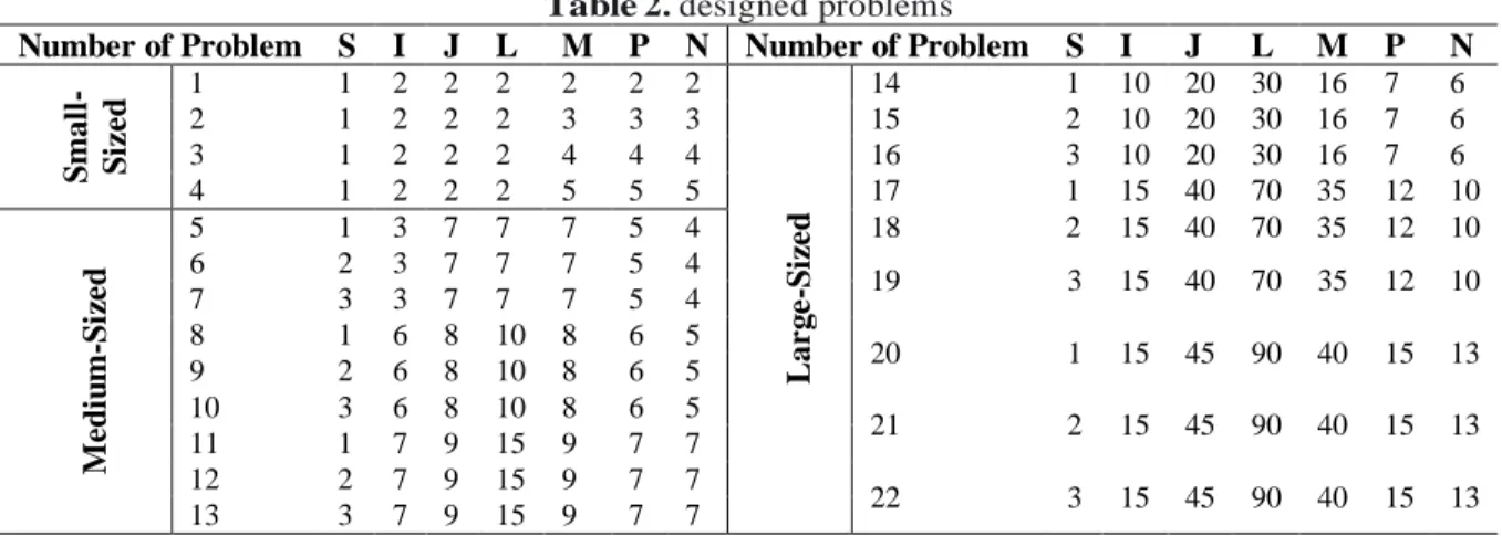
For the development of medium- and large-sized problems, a number of problems found in the relevant literature are reviewed. Next, with regard to the sizes mentioned in the literature, the size of medium and large problems and also a number of problems with a size larger than those in the previous studies are determined (Pishvaee et al., 2011, Wang & Hsu, 2010, Omidi-Rekavandi et al., 2014). The designed problems are presented in table 2., where S denotes the number of goods, I the number of manufacturing centers, J the number of distribution centers, L the number of customer centers, M the number of collection centers, p the number of recycling centers, and N the number of disposal centers.
Table 2.designed problems
Number of Problem S I J L M P N Number of Problem S I J L M P N
S
mal
l-S
iz
e
d
1 1 2 2 2 2 2 2
Lar
g
e
-S
iz
e
d
14 1 10 20 30 16 7 6
2 1 2 2 2 3 3 3 15 2 10 20 30 16 7 6
3 1 2 2 2 4 4 4 16 3 10 20 30 16 7 6
4 1 2 2 2 5 5 5 17 1 15 40 70 35 12 10
M
e
d
iu
m
-S
iz
e
d
5 1 3 7 7 7 5 4 18 2 15 40 70 35 12 10
6 2 3 7 7 7 5 4
19 3 15 40 70 35 12 10
7 3 3 7 7 7 5 4
8 1 6 8 10 8 6 5
20 1 15 45 90 40 15 13
9 2 6 8 10 8 6 5
10 3 6 8 10 8 6 5
21 2 15 45 90 40 15 13
11 1 7 9 15 9 7 7
12 2 7 9 15 9 7 7
22 3 15 45 90 40 15 13
13 3 7 9 15 9 7 7
4-3- Parameter setting
The algorithm parameters are set as follows:
• In the bee algorithm, the population size is equal to 200, watch bees accounted for 50% of the population, and the number of iterations in the parallel search algorithm is equal to 5.
• In the genetic algorithm, rates of 0.8 and 0.1 are considered for intersection and mutation, respectively, and the population size is estimated 150.
A study conducted by Pouralikhani et al. (2013) was taken as the basis for setting and initializing the model parameters. Since the model presented in their study did not cover some parameters of the model proposed in the present study, attempts are done to develop random which are logical compared to other values.
In order to develop triangular numbers associated with each fuzzy parameter (m1, m2, m3), m2 is first produced and then random number r is developed in the range of 0 and 1. Parameters m1 and m3 are also produced using equations m2*(1-r) and m2*(1+r), respectively. To initialize the fuzzy parameters, m2 is determined based on the aforementioned article [20] and m1 and m3 are determined in MATLAB. As a
result, only the value of m2 is mentioned in the development of these parameters. The following values are taken into account in the development of typical problems.
Table 3. Parameter setting
Parameter Range Parameter Range
𝑟̃𝑙𝑠𝑡 triangular fuzzy numbers of (m1, 10, m3) 𝑤𝑘 ~Uniform (1000,1600)
𝑑̃𝑙𝑠𝑡 triangular fuzzy numbers of (m1, 100, m3) 𝑤𝑐 2
𝑐𝑎𝑗 4000 𝑣𝑓 2
𝑓̃𝑝 triangular fuzzy numbers of(m1, 15000, m3) 𝑣𝑘 ~Uniform (70,100)
𝑓̃𝑛 triangular fuzzy numbers of (m1, 5000, m3) 𝛼𝑘 ~Uniform (0.1,0.2)
𝑓̃𝑚 triangular fuzzy numbers of(m1, 10000, m3) 𝑣𝑜𝑙𝑠 ~Uniform (1,20)
𝑓̃𝑗 triangular fuzzy numbers of(m1, 6000, m3) 𝑤𝑠 ~Uniform (1,20)
𝑝𝑓 1000 𝑝𝑐 500
All distances between centers are randomly developed in the same range [1, 50].
For ranking the fuzzy numbers, α is determined to be equal to 0.8.
4-4- Model validation results
In order to validate the model, the two-objective model is transformed into a single-objective model using the LP-metric method. The resulting single-objective model is then solved in GAMS for small-sized problems.
This study employed the LP-metric method which is popular in the literature study on multi-objective problems. Our goal is to minimize the deviations of the objective functions from their optimal value. In this method, individual solutions are first calculated for each of the objective functions, and then the following objective function is minimized:
min 𝑧 = [𝑤∗(𝑓
1(𝑥) − 𝑓1(𝑥∗))/𝑓1(𝑥∗)] + [(1 − 𝑤∗)(𝑓2(𝑥) − 𝑓2(𝑥∗))/𝑓2(𝑥∗)] (81)
where 𝑓1(𝑥∗) is the optimal solution of the first model by considering the first objective function, 𝑓2(𝑥) is
the value of the second objective function based on the optimal solution of the model obtained using only the first objective function, 𝑓2(𝑥∗) is the optimal value obtained from the solution of the model by taking
into account the second objective function, and 𝑓1(𝑥) is the value of the first objective function based on
the optimal solution of the model only using the second objective function. Moreover, 𝑤∗ is the weight of the objective functions.
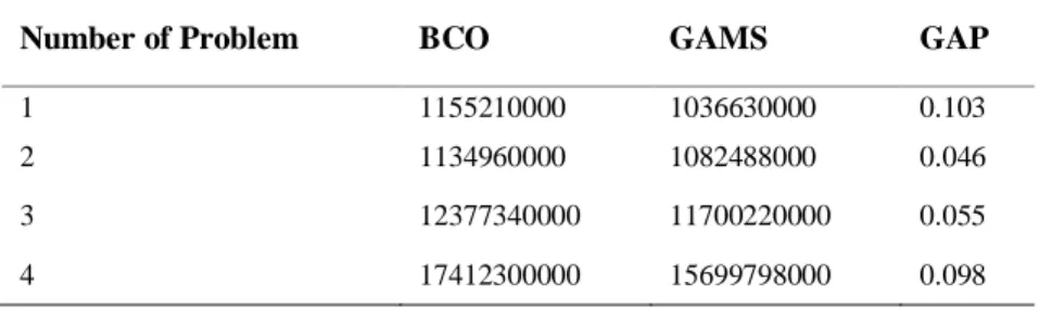
The presented model is programmed in GAMS and is solved using the BARON solver. In this method, the value of P is set to 1 and weight of the objectives is all considered 0.5. Small-sized problems are solved using the BCO algorithm and GAMS aiming to optimize the LP-metric method. The solutions of the small-sized problems solved using the proposed algorithms and GAMS are compared in table 4. As shown, the gap between the results of the BCO algorithm and GAMS is very small, indicating the validity of the algorithm and its convergence to the optimal or near-optimal solution.
Table 4. Solution results obtained using GAMS and BCO algorithm.
Number of Problem BCO GAMS GAP
1 1155210000 1036630000 0.103
2 1134960000 1082488000 0.046
3 12377340000 11700220000 0.055
4 17412300000 15699798000 0.098
In the above table, the gap between values is calculated using the following relation:
GAP =𝑂𝑏𝑗𝑒𝑡𝑖𝑣𝑒 𝑣𝑎𝑙𝑢𝑒𝐵𝐶𝑂− 𝑂𝑏𝑗𝑒𝑐𝑡𝑖𝑣𝑒 𝑣𝑎𝑙𝑢𝑒𝐺𝐴𝑀𝑆
𝑂𝑏𝑗𝑒𝑡𝑖𝑣𝑒 𝑣𝑎𝑙𝑢𝑒𝐵𝐶𝑂
4-5- Executive results
In this section, the developed experimental problems are solved using the bee colony and genetic algorithms and the results are analyzed. In the following table, the results of the two algorithms are shown in terms of comparative indices.
Table 5. The results of solving small-sized problems
Number of Problem
BCO GA
Quality Metric
S (Spacing Metric)
D (Diversity Metric)
Quality Metric
S (Spacing Metric)
D (Diversity Metric)
1 79.52 1.34 513.7 20.47 0.79 306.6
2 69.73 1.5 510.5 30.27 1.03 313.4
3 83.41 0.84 542.2 16.59 0.51 329.3
4 100 0.97 539.4 0 0.85 343.2
Table 6.The results of solving medium-sized problems.
Number of Problem
BCO GA
Quality Metric
S (Spacing Metric)
D (Diversity Metric)
Quality Metric
S (Spacing Metric)
D (Diversity Metric)
5 76.27 1.35 1399.1 23.73 1.03 969.1
6 87.13 0.98 3167.8 12.87 0.73 1931.4
7 88.76 1.11 4596.9 11.24 0.45 1671.7
8 96.99 1.05 4368.3 3.01 0.71 1857.2
9 81.99 0.81 2436.7 18.01 0.84 1643.7
10 75.79 1.25 3857.3 24.21 0.49 2245.7
11 92.11 0.58 4028.1 7.89 0.83 2784.5
12 91.41 0.84 4464.2 8.59 0.77 3740.5
13 100 1.07 7895.4 0 0.69 4540.7
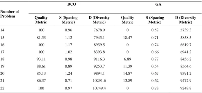
Table 7.The results of solving large-sized problems
Number of Problem
BCO GA
Quality Metric
S (Spacing Metric)
D (Diversity Metric)
Quality Metric
S (Spacing Metric)
D (Diversity Metric)
14 100 0.96 7678.9 0 0.52 5739.3
15 81.53 1.12 7945.1 18.47 0.71 5858.5
16 100 1.17 8939.5 0 0.74 6619.7
17 100 1.02 8393.8 0 0.66 6941.2
18 93.11 0.98 9116.3 6.89 0.77 8456.2
19 88.61 0.89 9253.7 11.39 0.54 8564.6
20 85.13 1.24 9894.1 14.87 0.67 9391.2
21 86.37 0.71 10291.6 13.89 0.62 9472.9
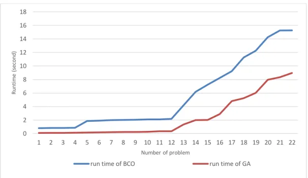
As can be seen in the above tables, in all small-, medium, and large-sized problems, values of quality and diversity indices obtained for the bee colony algorithm are greater than their corresponding values calculated through the genetic algorithm This suggests the higher ability and power of the bee colony algorithm in achieving the near-optimal solution and exploring its feasible region. In addition, the spacing metric showed that in most cases, the genetic algorithm searches the solution space in a more uniform manner. Figure 2 indicates that the runtime of problems in the bee colony algorithm is always longer than that of the genetic algorithm. In other words, the bee colony algorithm needs more time for solving these problems. It should be noted that as the size of the problem increases, the runtime increases too. Thus, the runtime of large-sized problems is longer than that of small- and medium-sized ones. This indicates the large-sized problems are hard problems. The following figure shows the comparison between the runtime of problems in the bee colony algorithm and the genetic algorithm.
Fig 2.Runtime comparison (seconds) 0
2 4 6 8 10 12 14 16 18
1 2 3 4 5 6 7 8 9 10 11 12 13 14 15 16 17 18 19 20 21 22
Ru
n
ti
m
e
(se
co
n
d
)
Number of problem
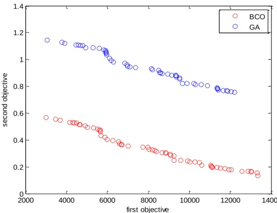
Fig 3. Pareto front for problem number 22 from large-sized problems
As shown in figure 3, the quality of solution obtained from the bee colony optimization (BCO) algorithm is higher than that of the genetic algorithm (GA). It also indicates that by reducing the second objective function, the first objective function increases and vice versa. This suggests the contradiction between the objective functions in the mathematical model proposed. In addition, the comparison between the Pareto front of the two algorithms demonstrates the good performance of BCO and its convergence towards optimal and near-optimal solutions.
5- Conclusion
The present study explored the robust optimization of PRP in a closed-loop supply chain aimed at reducing CO2 and CO emissions. In other words, this study sought to find a solution to simultaneously achieve robust optimization and carbon emission minimization in a closed-loop supply chain. In the proposed model, PRP is studied by considering the condition of simultaneous pickup and delivery of goods in the supply chain. To this end, a multi-objective robust optimization model is proposed and the bee colony and genetic algorithms are used to solve the model. Abased on the literature review, typical experimental problems are developed in three different sizes, namely, small, medium, and large, and the results obtained through the two algorithms are compared in terms of quality, diversity, spacing, and runtime. The results showed that the bee colony algorithm performs more efficiently in the exploration and extraction of the feasible region and finding near-optimal solutions. In terms of the spacing metric and runtime, the genetic algorithm had a better performance than the bee colony algorithm. In addition, the variations in runtime resulting from the increase in the problem size further confirmed that the studied problem is an NP-HARD problem.It is recommended to develop the present model in future studies by taking various aspects of sustainability into account (environmental, social, and economic). Moreover, uncertain parameters can be considered as combined, fuzzy, or probabilistic parameters. It is also recommended to adopt other approaches to solving the model and compare the results.
20000 4000 6000 8000 10000 12000 14000
0.2 0.4 0.6 0.8 1 1.2 1.4
first objective
s
e
c
o
n
d
o
b
je
c
ti
v
e
BCO GA
Acknowledgement
The authors would thank the Editor-in-Chief and the anonymous referees for their valuable comments to greatly improve the quality of this presentation.
References
Adulyasak, Y., Cordeau, J.-F. & Jans, R. (2014). Optimization-based adaptive large neighborhood search for the production routing problem. Transportation Science, 48(1), 20-45.
Adulyasak, Y., Cordeau, J.-F. & Jans, R. (2015). The production routing problem: A review of formulations and solution algorithms. Computers & Operations Research, 55, 141-152.
Bektas, T. & Laporte, G. (2011). The Pollution-Routing Problem. Transportation Research Part B: Methodological, 45(8), 1232-1250.
Deb, K., Pratap, A., Agarwal, S. & Meyarivan, T. (2002). A fast and elitist multiobjective genetic algorithm: NSGA-II. IEEE transactions on evolutionary computation, 6(2), 182-197.
Jimenez, M., Arenas, M., Bilbao, A. & Rodr, M. V. (2007). Linear programming with fuzzy parameters: an interactive method resolution. European Journal of Operational Research, 177(3), 1599-1609.
Kannan, G., Sasikumar, P. & Devika, K. (2010). A genetic algorithm approach for solving a closed loop supply chain model: A case of battery recycling. Applied Mathematical Modelling, 34(3), 655-670. Naber, S. K., Deree, D. A., Spliet, R. & Van-Den-Heuvel, W. (2015). Allocating CO2 emission to customers on a distribution route. Omega, 54, 191-199.
Omidi-Rekavandi, M., Tavakkoli-Moghaddam, R., Ghodratnama, A. & Mehdizadeh, E. (2014). Solving a Novel Closed Loop Supply Chain Network Design Problem by Simulated Annealing. Applied mathematics in Engineering, Management and Technology., 2(3), 404-415.
Pham, D., Ghanbarzadeh, A., Koc, E., Otri, S., Rahim, S. & Zaidi, M. The bees algorithm-A novel tool for complex optimisation. Intelligent Production Machines and Systems-2nd I* PROMS Virtual International Conference (3-14 July 2006), (2011). sn.
Pishvaee, M. S., Rabbani, M. & Torabi, S. A. (2011). A robust optimization approach to closed-loop supply chain network design under uncertainty. Applied Mathematical Modelling, 35(2), 637-649.
Pouralikhani, H., Najmi, H., Yadegari, E. & Mohammadi, E. (2013). A multi-period model for managing used products in green supply chain management under uncertainty. J. Basic Appl. Sci. Res, 3(2), 984-995.
Pradenas, L., Oportus, B. & Parada, V. (2013). Mitigation of greenhouse gas emissions in vehicle routing problems with backhauling. Expert Systems with Applications, 40(8), 2985-2991.
Sun, L. & Wang, B. (2015). Robust optimisation approach for vehicle routing problems with uncertainty. Mathematical Problems in Engineering, 2015, 1-8.
Taghavifard, M., Sheikh, K. & Shahsavari, A. (2009). Modified Ant Colony Algorithm For The Vehicle Routing Problem With Time Windows. International Journal of Industrial Engineering and Production Management, 20(2), 23-30.