yongsuan.pdf

(1)

Yongsu An. The impact of the MERS Outbreak in Daily Lives: Sentiment Analysis of Korean Tweets using Time-series Methods. A Master’s Paper for the M.S. in I.S degree. April, 2016. 35 pages. Advisor: Jaime Arguello

This study examines the correlation between sentiments in tweets and the number of passengers in the subway as the social index during the MERS outbreak in South Korea. The observation that motivated this study in the social context was that people tended to avoid their social lives outdoors by the fear of being infected during the situation. Two time-series datasets were processed for the purpose of getting rid of seasonal patterns. The result showed that they are correlated with each other with 169 hours. It indicates that the sentiments in social media can be a good way of mirroring people’s behaviors ahead of time.

Headings:

Text mining

Sentiment analysis

(2)

THE IMPACT OF THE MERS OUTBREAK IN DAILY LIVES: SENTIMENT ANALYSIS OF KOREAN TWEETS USING TIME-SERIES METHODS

by Yongsu An

A Master’s paper submitted to the faculty of the School of Information and Library Science of the University of North Carolina at Chapel Hill

in partial fulfillment of the requirements for the degree of Master of Science in

Information Science.

Chapel Hill, North Carolina

April 2016

Approved by

(3)

List of Tables

Table 1. The number of world-wide cases and deaths against MERS ... 5

Table 2. Dates and important events in the MERS timeline ... 7

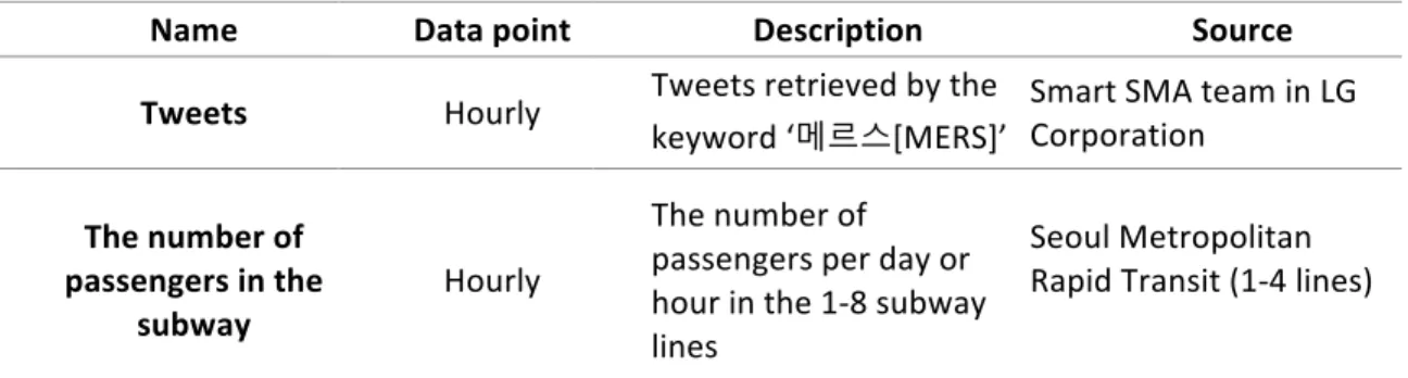
Table 3. The overview of the datasets ... 13

Table 4. The examples and descriptions of the disease-related words ... 21

List of Figures

Figure 1. The number of cases and deaths against MERS in South Korea ... 6

Figure 2. The number of tweets in the period of the MERS outbreak ... 15

Figure 3. The number of passengers in 2014 and 2015 on a daily basis ... 16

Figure 4. The number of passengers in 2015 on an hourly basis ... 16

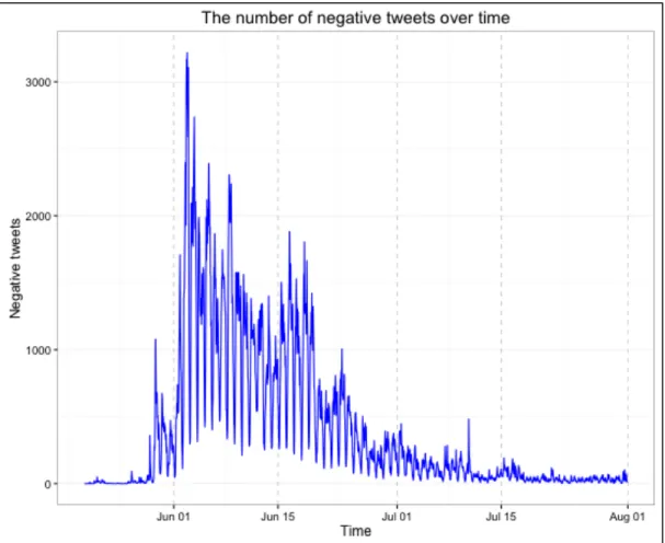
Figure 5. The number of negative tweets in the period of the MERS outbreak ... 19

Figure 6. The number of disease-related words in the period of the MERS outbreak ... 20

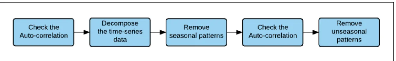
Figure 7. The white-noisening process ... 22

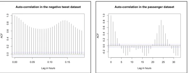
Figure 8. The auto-correlation result of the negative tweet dataset ... 23

Figure 9. The auto-correlation result of the passenger dataset ... 23

Figure 10. The decomposition result of the passenger dataset ... 24

Figure 11. The decomposition result of the negative tweet dataset ... 24

Figure 12. The auto-correlation result of the passenger dataset after removing seasonal and unseasonal correlations ... 26

Figure 13. The auto-correlation result of the passenger dataset after removing seasonal and unseasonal correlations ... 26

Figure 14. The plot of the passenger dataset after removing seasonal and unseasonal correlations ... 26

Figure 15. The plot of the negative tweet dataset after removing seasonal and unseasonal correlations ... 26

Figure 16. The cross-correlation value with lag values between the disease-related words and the social index ... 28

(5)

1. Introduction

Social media has become a place where people express their opinions and share the

information in real time. The extensive amount of microbloggings by users enables

researchers to collect and analyze the huge datasets. Political and economic organizations

are also paying attention to the possibility of social media analysis to monitor people’s

feedbacks. This is because the opinions and information uploaded by people are a lively

feedback of their products or policies in real time.

The sentiment analysis is one of research topics in social media analysis that aims to

explore people’s opinions on specific topics. Many approaches have been made to

identify the best features that represent the map of people’s feeling revealed in social

media. While many researchers classified the opinions into negative and positive one,

other researches tried to split it by several moods that consist of human’s dominant

feelings.

Social media is also a place during the crisis situation such as natural disasters, epidemic

diseases where people share up-to-date information about the situation, or their feelings.

Especially, in epidemic situation, we can monitor the social media to observe and reflect

(6)

2. Background

2-1. About Middle East Respiratory Syndrome

Historically, epidemic diseases have swept over the society with great impact on it. There

have been also few huge sweeps in the recent few decades throughout the world: SARS,

H1N1. These outbreaks usually caused serious damages - Many people were sacrificed

by them, and a long-term pandemic led to a huge disruption to the society.

Middle East Respiratory Syndrome(MERS) is a viral respiratory illness which was first

reported in Saudi Arabia in 2012. Also known as camel flu, it has been identified to come

from some viruses in the body of camels, according to the World Health Organization

(2015). All of the cases at the first stage are known to be infected through their travels or

visits in countries near Arabian Peninsula. The symptoms of this disease include fever,

cough, and shortness of breath, which falls in the category of respiratory symptom.

MERS is to be also featured as having the 2-14 days of the incubation period. Some cases

go through severe complications, whereas some just recovered from it after mild

(7)

2-2. Timeline of MERS throughout the world

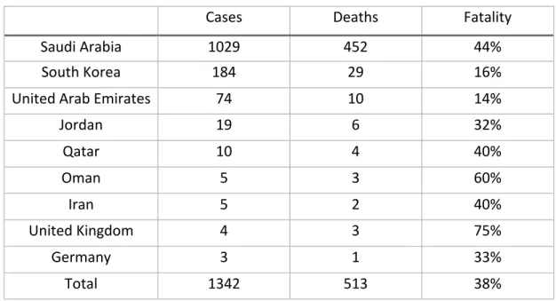
Table 1. The number of world-wide cases and deaths against MERS

Cases Deaths Fatality

Saudi Arabia 1029 452 44%

South Korea 184 29 16%

United Arab Emirates 74 10 14%

Jordan 19 6 32%

Qatar 10 4 40%

Oman 5 3 60%

Iran 5 2 40%

United Kingdom 4 3 75%

Germany 3 1 33%

Total 1342 513 38%

Note: Reprinted from European Centre for Disease Prevention and Control. Severe respiratory disease associated with MERS-CoV, by Stockholm: ECDC, Retrieved from

MERS had widely spread throughout some countries in the Arabian Peninsula at the

beginning stage. Table 1 shows the number of cases and deaths against MERS throughout

the world. The first considerable surge in the number of cases occurred in Saudi Arabia,

where 282 MERS-related deaths out of 688 cases were reported in 2012 (WHO, 2015). In

the United States, a man who came back from the travel to Saudi Arabia was reported as

the first case. After few more cases were reported, however, the Centers for Disease

Control and Prevention (CDC) (2015) successfully terminated the situation without any

(8)

As of June 2015, 1227 cases were reported to WHO (2015) along with 449 deaths at 37%

fatality rate. 28 countries reported the cases, while most of cases lie in three countries,

Saudi Arabia, South Korea, United Arab Emirates. While no case has been recently

reported throughout the world after the MERS outbreak in South Korea in 2015, MERS

is known as one of serious epidemics due to its considerable fatality rate.

2-3. MERS in South Korea

(9)

South Korea is the only place where the considerable number of cases was reported

outside of the middle east Asia. MERS was first introduced in South Korea by a

businessman who visited Saudi Arabia, United Arab Emirates and Bahrain. The health

authority failed to report the first case on time, which led to the serious outbreak

throughout the whole country. Figure 1 visualizes the number of cases and deaths against

MERS in South Korea.

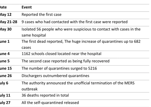
Table 2. Dates and important events in the MERS timeline

Date Event

May 12 Reported the first case

May 21-28 9 cases who had contacted with the first case were reported

May 30 Isolated 56 people who were suspicious to contact with cases in the same hospital

June 1 The first dead reported, The huge increase of quarantines up to 682 cases

June 4 1162 schools closed located near the hospital

June 5 The second case reported as being fully recovered

June 15 The number of quarantines surged to 5216

June 26 Dischargers outnumbered quarantines

July 6 The authority announced the unofficial termination of the MERS outbreak

July 11 36 deaths reported in total

July 27 All the self-quarantined released

(10)

After the first case was reported on May 20, a sharp increase in the number of cases

brought the attention to this disease. June 1 is one of important dates in the timeline when

the first death was reported, and the number of quarantines showed a huge spike up to

682 cases. This increasing trend in the statistics began to slow in late June. This outbreak

was unofficially terminated on July 6 with 36 deaths reported in total.

2-4. Research questions

Putting all backgrounds together, this paper would like to examine those questions in the

quantitative methods as follows:

• What would be the features to represent people’s feelings reflected in tweets?

• Does the sentiment analysis about MERS on Twitter correlate to the statistic of

passengers in the subway? What is the relationship between them revealed by

time-series analysis?

• Does the correlation help to describe people’s feelings and behaviors to avoid

(11)

3. Literature review

3-1. Online Social Network analysis based on time-series data

Many researches on sentiment analysis in Online Social Network (OSN) have been

examined to observe the public mood. A Time series is especially a type of dataset which

helps us to capture the changes of features along with the social phenomenon over time.

The trend of any given dataset in the timeline also can contribute to forecasting the

changes in the near future.

3-2. Correlation between the sentiment in OSN and the social index

The sentiment analysis from the large-scale of text datasets is becoming more and more

prevalent methods with machine-learning techniques. As extensively reviewed by Pang

and Lee (2008), a variety of methods in the category of the supervised and unsupervised

techniques have been developed by researchers in this field. Nagy and Stamberger (2012)

investigated the sentiment in tweets during the California gas explosion on September

2010 with a trained model in supervised methods. They analyzed 3698 tweets which were

manually annotated by a crowdsourcing system, then compared 4 different systems:

SentiWordNet, AFNN, Bayesian Network, and combination of emoticons with either of

three approaches. Many researchers use supervised approaches by feeding an annotated

dataset based on the gold standard and training the classifier to predict the classification

of unseen data. The unsupervised technique, on the other hand, focuses on the similarity

(12)

researches which applied a TF-IDF weighting method and k-means algorithm to score

and cluster positive and negative documents. Clustering-based unsupervised approaches

have the advantages over the supervised approach in that they are flexible to analyze a

large-scale dataset without having to involve human in annotating the dataset.

The sentiment analysis in OSN is a useful method to analyze the social phenomena.

Researches on this topic often use social indices from a various of social sectors as

counterpart measures to represent a cross section of the society. A variety of topics in

political, economic sectors, and also crisis situations have been observed with the

sentiment analysis. Thelwall et al. (2011) analyzed the reaction of people in social media

against a set of general events in the United States by classifying the events into positive

and negative one. The trends of the 30 largest spiking events in tweets showed that huge

increases in negative sentiments tend to indicate the big events extensively mentioned in

Twitter.

Some researches on the relationship between social indices and the sentiment in OSN

have been trying to figure out how the sentiment analysis is useful to predict social

phenomena. One of dominant social sectors that are examined by researchers are

economic situations. While there are few social indices which can represent the economic

status, the stock index is a good measure to bring in the economic status extensively used

by many researches. Bollen et al. (2011) examined the correlation between the Dow

Jones Industrial Average (DJIA) and the public mood in tweets. Grander causality

(13)

at a significant level. This method examines the causal relationship between two time

series that may have a temporal lag. It also enables us to claim that one time-series

influences the change of another time-series afterwards. They classified the sentiment

into 6 different mood states as well as divided it in the bipolar classifier. This approach

demonstrated how we can take a closer look at the emotions in the macro-level of

classification.

On the contrast to the predictive analysis, the descriptive analysis takes up another

portion of researchers associated with social indices. It differs from the predictive

analysis in that it tries to expose meaningful correlations between the social index and the

sentiment in OSN. It assumes that OSN well reflects on people’s feelings as a mirror of

the society. Lansdall et all. (2012) developed their study on tweets in the period of the

recession in the United Kingdom from 2009 to 2012. It described that the difference in

mean for the 50 days before and after the main events in UK fluctuated along with the

events that resulted in the economic downturn. Anger and fear, especially indicated an

increase during the period of the recession.

Political event is of another concern which many people greatly pay attention to. The

political statistics such as election results, polls about politicians, parties, and their

policies have had always an important role in predicting the future of the society.

O’Connor et al. (2010) examined how the sentiment as a reflection of people’s opinions

is correlated to the polls on economic status and political preferences. Four polls were

(14)

smoothing made different correlation rates, while it turned out that sentiment ratio

captures the trends of confidence surveys and presidential elections poll in 2008.

3-3. Crisis situation

Social media analysis in crisis situations is another area where researchers have paid

more attention to. Twitter, especially, have an informative role in spreading up-to-date

information in the situation when real-time notification is critical to prevent the situation

from being worse. The sentiment analysis in crisis situations can be an indicator of how

the crisis actually affects the public mood and their lives, and thus can be used to come

up with follow-up measures.

Salathe et al. (2011) focused on the dynamics of health behaviors reflected in Twitter.

They resulted from the analysis on six-month period of the H1N1 outbreak that there is a

significant correlation between sentiments in tweets and CDC-estimated vaccination rate

by region. The network and community detection, which is another part of this study,

indicated that users on Twitter tend to share the same sentiment, positive or negative, and

form their own communities. Chew et al. (2010) also analyzed the H1N1 outbreak

focusing on the content analysis. They manually classified 5395 tweets into several types

of contents in terms of content, qualifiers, and links. Resource-related posts and news

website were mostly shared by people indicating that Tweets can play valuable role in

(15)

4. Data

This research explores two time-series datasets for the analysis: Tweets, and social

indices. The summary of the datasets is given in Table 3. All datasets base its data points

on an hourly basis with 1752 data points. This research, which aims to examine the

correlation between tweets and the social index, covers the whole main period of the

MERS situation in South Korea. The starting point of the dataset was set for May 20

when the public started to react to the outbreak in Twitter. For the end point of the

dataset, Jul 31, when the outbreak was stabilized and the authorities announced unofficial

termination of the situation, was assumed to be appropriate.

The social index used in this research is the public transportation statistics obtained from

Seoul Metropolitan Rapid Transit (SMRT) Corporation. This dataset indicates the

number of passengers in the subway of line 1-4 in Seoul in the given time. Almost 20

million people, which is the half of the Korean population, reside in the metropolitan of

Seoul. The subway is the most popular and important transportation for commutes and

travels. 3.2 billion of people, according to the statistic provided by SMRT (2014), use the Name Data point Description Source

Tweets Hourly Tweets retrieved by the keyword ‘메르스[MERS]’

Smart SMA team in LG Corporation

The number of passengers in the

subway Hourly

The number of passengers per day or hour in the 1-8 subway lines

Seoul Metropolitan Rapid Transit (1-4 lines)

(16)

subway in 2014. Since the 1-4 line takes up more than 50% of the whole passengers in

the subway, the dataset is worth representing the population of subway passengers in

Seoul, South Korea.

4-1. Tweets

About 850,000 Korean tweets were collected with the keyword ‘메르스’[MERS]. This

dataset may not include tweets which mention about the MERS situation without the

keyword, but the only one keyword was considered as a search keyword to avoid noises

coming into the dataset. The tweet dataset is comprised of several columns: “doc id”,

“url”, “crawled date”, “published date”, “title’, “comment count”, and “content”. The

(17)

Figure 2. The number of tweets in the period of the MERS outbreak

Few important turning points are annotated in Figure 2. It starts with almost only few

tweets in late May at the beginning stage of the outbreak. The first case was reported on

May 20, and thus the people began to be aware of the existence of this disease. A sudden

surge in tweets is shown on June 1 when the first death was reported. It seems that the

report of actual victim brought to people that this disease could threaten the safety. It

almost increased up to 4500 tweets per hour at the peak. Most of contents at this time

mention about their worries or retweet the updated news from the press. After this

(18)

Another noticeable increase in tweets can be seen on June 17 when the number of

quarantines has topped 6,729. In July, this fluctuation is gradually stabilized starting from

the early July, then only few tweets were detected at the end of the given period on the

hourly basis.

4-2. Passengers in subway

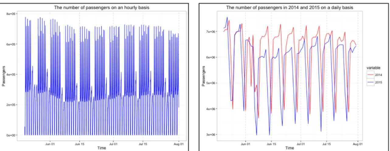
Figure 3. The number of passengers in 2015 on an hourly basis

Figure 4. The number of passengers in 2014 and 2015 on a daily basis

Figure 4 describes the number of passengers in the given period in 2014 and 2015. The

daily and hourly datasets were plotted for the better understanding of how it changed. In

the daily passenger dataset, the statistic of 2015 in passengers in comparison with the one

of 2014 starts to decrease on June 6. It almost drops down to 85% of one in 2014, and

then begins to recover its losses throughout July. When compared to tweet dataset along

(19)

While the first victim was reported on June 1 with the biggest surge in tweets, the change

in passengers has been captured few days later.

4-3. Data Preparation

Texts in tweet dataset were tokenized and parsed in the following procedure:

1. Removal of useless parts of texts (url, hashtags, user tags)

2. Tokenization of all words by white space

3. Annotation of part-of-speech tags

After removing urls, hashtags, user tags, which are usually considered as less important

parts of texts, the following steps were carried out using KonPy, a natural language

processing API package for Korean implemented in Python. The set of APIs has different

APIs in itself that work in different ways. One of the APIs, named ‘Twitter API’, which

is more sensitive to detect non-spaced terms, was used in this research. The important

issue in natural language processing for Korean is to address the problem of the word

segmentation

1) ‘아버지가방에들어가신다’

2) ‘아버지가 방에 들어가신다’

(20)

In the example above, the second sentence is an example of well-formed Korean text

with appropriate space between them. However, users on the internet tend not to take care

of spacing words since they usually type in their words by smartphones, tablets in many

occasions. The first sentence results from this typing behavior, even though it still makes

sense to deliver the meaning of words. In this case, APIs should be tweaked to well detect

each word in the non-spaced text. For this reason, the ‘Twitter’ API was selected to deal

with this issue usually found in tweets.

5. Methods

5-1. Features

After the part-of-speech tagging, the next issue is to select which part-of-speeches will be

used to determine the sentiment of tweets. We focused only on adjectives and verbs,

based on the assumption that other parts of speech are less likely to convey positive or

negative sentiment.

All adjectives and verbs were judged by a Korean sentiment API named OpenHangul

(2014). The sentiment analysis in the paper used the simple majority vote to determine

the sentiment of tweets, positive and negative. For example, if a tweet has 3 positive

(21)

A. Feature 1: Negative tweets

Figure 5. The number of negative tweets in the period of the MERS outbreak

The first feature used for the analysis is the number of negative tweets per hour. The

negative tweets in each hour were counted to figure out how many negative tweets were

published at the given hour. Figure 4 shows the trend of the number of negative tweets on

an hourly basis. The number of positive tweets was put together to easily compare how

(22)

B. Feature 2: Disease-related words

Figure 6. The number of disease-related words in the period of the MERS outbreak

The next feature deals with disease-related words to capture how people feel and how

they actually express their feelings toward the disease. Few examples of disease-related

terms are listed in Table 4. While sentiment words such as “fear”, “anxious”, “worried”

come into play as features, some words that describe the situation such as “spread”,

“transfer” but does not necessarily have feelings, can reveal that people want to share the

(23)

Description Example

Describe how the disease goes on 퍼지다[PeoJiDa; spread], 옮기다[OmGiDa; infected]

Express fearful feelings 무섭다[MuSeobDa; scary], 걱정[GeokJeong; worry],

위기[WeGi; crisis], 충격[ChoongGeuk; shock]

Describe the symptoms of the

disease 아프다[APeuDa; hurt], 걸리다[GeolLiDa; catch]

Criticize the authorities 무능하다[MuNeungHaDa; incapable]

Table 4. The examples and descriptions of the disease-related words

The trend of this feature looks similar in the most parts. The number of words suddenly

surges on early June, which lead to the downward trend over time.

C. Feature 3: The ratio of Negative and Positive tweets

The ratio of negative and positive tweets was examined as the last feature. However, this

feature turned out to be vulnerable to the number of tweets by the fact that the sparse

dataset at the very first and the last part of the dataset leads to unstable fluctuation of the

(24)

Figure 7. The white-noisening process

5-2. Removal of seasonal patterns

The analysis of time-series data always accompanies the issue of seasonal patterns. Many

statistics such as natural phenomenon, behavioral patterns of people are inevitable to be

affected by time periods. For example, in the case of the number of tweets, we can

naturally speculate that people are likely to publish more tweets during the day, whereas

less tweets are published in the early hours of the morning. This hourly pattern is actually

detected in both time-series data shown in Figure 4 and 5. These hourly fluctuations are

easily shown in the time-series datasets since tweets and passengers are counted on an

hourly basis. Some daily and monthly patterns may also exist in these datasets as well. In

other words, more people are likely to use public transportations during the week for their

commutes whereas this trend is likely to be opposite during the weekend. Therefore,

these seasonal trends should be removed before the correlational analysis of time-series

datasets. The entire process of the white-noisening process is visualized in Figure 7. The

following tasks were processed using R programming:

1. Transform the data into time-series formatted dataset

2. Check auto-correlation

(25)

Figure 8. The auto-correlation result of the negative tweet dataset

Figure 9. The auto-correlation result of the passenger dataset

The datasets first need to be transformed to the time-series format such that the R

programming identifies the dataset to operate appropriate time-series analysis in the

following steps. After that, the auto-correlation function verifies the correlation between

data points. Each data point is compared with each other with k-time lags. As shown in

Figure 6 and 7, the x axis indicates that data at time n and at time n+k is tested to see their

correlations with the lag of time k. All the y values go beyond the blue line, meaning that

they are significantly correlated to each other. In other words, the repeated time interval

affects the correlation of data points, which harms the assumption that each data point in

the same dataset should be independent of each other without being affected by seasonal

components. Judged by the auto-correlation testing, it turns out that the seasonal pattern

(26)

Figure 10. The decomposition result of the passenger dataset

Figure 11. The decomposition result of the negative tweet dataset

The next step is to decompose the dataset to handle the seasonal component. The stl

function in the R programming allows us to automatically detect patterns with the regular

time interval. Figure 10 reveals that a daily peak in passengers is observed. This weekly

pattern is easily detectable which is comprised of five sharp peaks during the week and

two moderate peaks during the weekends. All these seasonal patterns are detected and

thus end up being stripped away. The trend part in Figure 9 and 10 represents a

visualization of how this time-series data changes over time. Figure 9 displays a sudden

drop and moderate increase in the number of passengers.

This research exploits only the remainder part of the decomposition to measure the

cross-correlation with another time-series data. The formula to draw the random part of the

(27)

Remainder = data - seasonal - trend

A notable part of the remainder data in passengers is a sharp drop to the baseline on May

20. The day is the one and only holiday in the given period, which led to a considerable

decrease in the number of passengers. The rest of part doesn’t seem to display any regular

patterns.

5-3. Removal of unseasonal patterns

However, the auto-correlation on the dataset after the decomposition still has some

significant correlations. This is because, while some patterns are repeated on regular

interval, some non-repeated correlations still possibly remain. For example, if there is a

correlation of 11 days between June 1 to 11, and July 1 to 11, it will not be detected

because it is not periodically repeated. This correlation is just repeated twice, not

periodically throughout the whole period. In this case, this correlation is not detected as

(28)

Figure 12. The auto-correlation result of the passenger dataset after removing seasonal and unseasonal correlations

Figure 13. The auto-correlation result of the passenger dataset after removing seasonal and unseasonal correlations

Figure 14. The plot of the normalized passenger dataset after removing seasonal and unseasonal correlations

(29)

ARIMA function is a well-known function to white-noisen the time-series data.

White-noisening the data, which means the time-series data should not include the correlation

between data points within itself, should be processed before doing cross-correlation.

Figure 14 and 15 of the auto-correlation plot shows that almost all the correlated part

ended up being removed after applying ARIMA function.

6. Result

6-1. Pearson-correlation

Pearson correlation measures linear correlation between two variables. If the two datasets

in the given time are correlated each other, the correlation value will be within -1 to 1,

except for zero meaning that they are independent. Two features turned out to be

significantly correlated to the social index where the p-value is less than 0.05. The

correlation value of the number of diseases-related words were a bit higher than the one

for the number of negative tweets.

6-2. Cross-correlation with two time-series data

However, Pearson correlation does not consider the changes over time. All the data

points in the timeline are assumed to be independent, which makes it impossible to

speculate the relationships over time. It is still meaningful to look at their relationship in

the independent setting, but the changes over time are expected to tell us more about their

(30)

for this limitation. This metric also enables us to see how two series of data are correlated

as one of them are lagged relative to another. If it turned out that they are more correlated

to each other at a lag of n, it means that X after n time slot is statistically meaningful to Y

at time 0.

Figure 16. The cross-correlation value with lag values between the negative tweets and the social index

Figure 17. The cross-correlation value with lag values between the disease-related words and the social index

These two plots show how correlation value changes at the different time lags. If the lag

is 500 with the positive y value 0.21, for example, the number of sentiment tweets (x

value) ahead of 500 hours can be said to be highly correlated to the number of subway

passengers (y value) at time 0. As seen in the chart, the correlation value with a little time

lag is higher than the one at time 0. The correlation value went to the peak of 0.195 at the

lag of 169 hours (8 days + 1 hour) with the number of negative tweets, and 0.212 at the

(31)

7. Discussion & Conclusion

This research aimed at analyzing the usefulness of the sentiment analysis to reveal the

public mood in the MERS outbreak. As revealed in papers in social network analysis, a

large scale of text dataset turned out to be useful enough to represent the feeling of the

public. As shown in the previous section of this paper, the number of negative tweets

revealed in the tweet dataset showed multiple spikes associated with important events in

the outbreak. The correlation analysis between text features and the social index also

indicated that the trend of features significantly has a negative relationship with the

number of passengers. It indicates that analyzing the social media is a meaningful way of

observing a society and people’s behavior.

In terms of the characteristic of the social event examined in this study, the epidemic

situation is one of the primary research areas in social media analysis. It is important to

look at how people feel about the situation, and also how information about the disease

spread over social media users in the outbreak situation. Some misinformation is likely to

make the situation more unstable, and some up-to-date information needs to be

disseminated, so it is obvious that information diffusion process really matters in these

crisis situations. The sentiment analysis will be able to give the authorities and relevant

organizations to make decisions on upcoming policies.

This paper especially focused on how the public mood revealed in tweets leads to the

behaviors of not going outside by the fear of being infected by looking at public

(32)

and the trend of text features in tweets proved it to be statistically significant. The result

specifically indicated that the negative mood in tweets has brought to realization of the

decrease in the number of subway passengers. It cannot be said that they are in the causal

relationship, but at least it proved that the sentiment analysis in OSN is an indicator of

people’s behavior in the near future.

Several open questions still remain for the future work. First, much more detailed mood

classification can be possibly examined to enrich the aspects of the research. This

research assumed that the public mood is judged as positive or negative by the majority

vote, which still makes meaningful implications but not enough to specify the types of

feelings. This mood analysis was beyond the ability of this study due to a lack of tweets

per hour in the dataset. Second, the disease-related words, which is the second feature of

text analysis, can be judged by more credible sources, for example, a corpus for

disease-related words. Developing a corpus of disease-disease-related words and verifying it against a

crisis situation will be able to elicit additional implications in this area of the study.

Third, in terms of text features, a diversity of features and technique can bring more

interesting results. In case that the dataset is judged by the binary classifier which assigns

0 or 1 when the number of tweets is going upward or downward, then the research will

form the discrete data analysis. Additional interesting features will also need to come into

play to validate the multiple dimension of the MERS outbreak.

The process of the time-series data analysis was another part of this study which required

(33)

affected by time, the issue of getting rid of seasonal patterns needed to be addressed prior

to the correlation analysis. The hourly data especially required multiple seasonal patterns,

on an hourly, daily, weekly basis, to be removed. Nevertheless, it is obvious that the

time-series analysis is a valuable and useful approach to identify how the data has

(34)

8. Bibliography

Bollen, J., Mao, H., & Zeng, X. (2011). Twitter mood predicts the stock market. Journal of Computational Science, 2(1), 1-8.

Bollen, J., Pepe, A., & Mao, H. (2009). Modeling public mood and emotion: Twitter sentiment and socio-economic phenomena. arXiv preprint arXiv:0911.1583.

Chew, C., & Eysenbach, G. (2010). Pandemics in the age of Twitter: content analysis of Tweets during the 2009 H1N1 outbreak. PloS one, 5(11), e14118.

Culotta, A. (2010). Detecting influenza outbreaks by analyzing Twitter messages. arXiv preprint arXiv:1007.4748.

Fung, I. C. H., Fu, K. W., Ying, Y., Schaible, B., Hao, Y., Chan, C. H., & Tse, Z. T. H. (2013). Chinese social media reaction to the MERS-CoV and avian influenza A (H7N9) outbreaks. Infectious diseases of poverty, 2(1), 1-12.

Gilbert, E., & Karahalios, K. (2010, May). Widespread Worry and the Stock Market. In ICWSM (pp. 59-65).

Lansdall-Welfare, T., Lampos, V., & Cristianini, N. (2012, April). Effects of the Recession on Public Mood in the UK. In Proceedings of the 21st international conference companion on World Wide Web (pp. 1221-1226). ACM.

Li, G., & Liu, F. (2010, November). A clustering-based approach on sentiment analysis. In Intelligent Systems and Knowledge Engineering (ISKE), 2010 International

Conference on (pp. 331-337). IEEE.

Nagy, A., & Stamberger, J. (2012, April). Crowd sentiment detection during disasters and crises. In Proceedings of the 9th International ISCRAM Conference (pp. 1-9).

O'Connor, B., Balasubramanyan, R., Routledge, B. R., & Smith, N. A. (2010). From Tweets to Polls: Linking Text Sentiment to Public Opinion Time Series. ICWSM, 11(122-129), 1-2.

(35)

Salathé, M., & Khandelwal, S. (2011). Assessing vaccination sentiments with online social media: implications for infectious disease dynamics and control. PLoS Comput Biol, 7(10), e1002199.

Seoul Metropolitan Rapid Transit. (2015). Open data API. Retrieved from http://data.seoul.go.kr/openinf/dataset/datasetlist.jsp

Shi, W., Wang, H., & He, S. (2013). Sentiment analysis of Chinese microblogging based on sentiment ontology: a case study of ‘7.23 Wenzhou Train Collision’. Connection Science, 25(4), 161-178.

The Ministry of Health and Welfare in South Korea. (n.d.). The Domestic status of cases and quarantines in the MERS outbreak. Retrieved from

http://www.mers.go.kr/mers/html/jsp/Menu_B/content_B1.jsp

The Center for Disease Control and Prevention in the United States. (2015). MERS in the U.S. Retrieved from http://www.cdc.gov/coronavirus/mers/us.html

Thelwall, M., Buckley, K., & Paltoglou, G. (2011). Sentiment in Twitter events. Journal of the American Society for Information Science and Technology, 62(2), 406-418. Pang, B., & Lee, L. (2008). Opinion mining and sentiment analysis. Foundations and trends in information retrieval, 2(1-2), 1-135.

World Health Organization (WHO). (2015). Middle East respiratory syndrome coronavirus (MERS-CoV). Retrieved from