Artificial Neural Networks, Support Vector
Machine and Energy Detection for Spectrum
Sensing based on Real Signals
Mohammed Saber
1,2, Abdessamad El Rharras
1, Rachid Saadane
1, Hatim Kharraz Aroussi
2and Mohammed Wahbi
11Laboratory Engineering system, SIRC/LAGeS-EHTP, Hassania School of Public Works, Casablanca, Morocco 2Laboratory Information Modeling and Communication Systems (IMCS), Ibn Toufail University, Kenitra, Morocco
Abstract: A Cognitive Radio (CR) is an intelligent wireless communication system, which is able to improve the utilization of the spectral environment. Spectrum sensing (SS) is one of the most important phases in the cognitive radio cycle, this operation consists in detecting signals presence in a particular frequency band. In order to detect primary user (PU) existence, this paper proposes a low cost and low power consumption spectrum sensing implementation. Our proposed platform is tested based on real world signals. Those signals are generated by a Raspberry Pi card and a 433 MHz Wireless transmitter (ASK (Amplitude-Shift Keying) and FSK (Frequency-Shift Keying) modulation type). RTL-SDR dongle is used as a reception interface. In this work, we compare the performance of three methods for SS operation: The energy detection technique, the Artificial neural network (ANN) and the support vector machine (SVM). So, the received data could be classified as a PU or not (noise) by the ED method, and by training and testing on a proposed ANN and SVM classification model. The proposed algorithms are implemented under MATLAB software. In order to determine the best architecture, in the case of ANN, two different training algorithms are compared. Furthermore, we have investigated the effect of several SVM functions. The main objective is to find out the best method for signal detection between the three methods. The performance evaluation of our proposed system is the probability of detection (𝑷𝒅) and the false alarm probability (𝑷𝒇𝒂). This
Comparative work has shown that the SS operation by SVM can be more accurate than ANN and ED.
Keywords: Cognitive radio, spectrum sensing, energy detection, artificial neural networks (ANN), support vector machine (SVM), Raspberry Pi 3, 433 MHz Wireless transmitter, RTL-SDR.
1.
Introduction
The already existed radio resources are becoming increasingly in demand, because of the wireless communication emergence (wireless technologies and its various services). Under a static frequency spectrum allocation, a study carried out by the Federal Communications Commission (FCC) [1] has shown that the frequency spectrum use is not regular; according to the different times and the geographical position; some frequencies bands are not occupied or partially occupied and others are highly demanded [1, 2], the activity is concentrated on cellular radio and FM bands. The unused frequencies have been termed as spectrum holes. A spectrum hole is a region of spatiotemporal frequencies assigned to a licensed user (primary users ‘PU’), but, at a particular time and specific geographic location, the band is not being utilized by the PU wherein a secondary and unique use is possible. As a conclusion of this previous study, FCC recommends an efficient spectrum management and access to enhance the spectrum efficiency, and specifies that unlicensed devices should have the capability of identifying free bands.
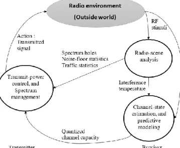
In order to reduce the waste of spectrum resources and increase the spectral efficiency, the concept of cognitive radio (CR) was introduced and proposed by Joseph Mitola in 1999 [3, 4]. The CR is defined as an intelligent device that senses the spectrum holes and makes it available for unlicensed users (secondary users (SU)). In CR the SUs can take advantage of these spectral holes dynamically and opportunistically, without causing any harmful interference to PUs. CR is a concatenation of software defined radio and artificial intelligence, with the aim of providing an efficient spectrum usage, also defined by FCC as: “A radio or system that senses its operational electromagnetic spectrum environment and can dynamically and autonomously adjust its radio operating parameters to modify system operation”. Figure 1 illustrates a basic cognition cycle model as introduced by Haykin [5].
Figure 1. Basic cognitive cycle. (The figure focuses on three fundamental cognitive tasks.)
International Journal of Communication Networks and Information Security (IJCNIS) Vol. 11, No. 1, April 2019 signal energy exceeds the threshold, we declare the presence
of the PU, otherwise it is absent.
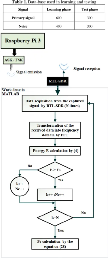
During the last years soft computing techniques like artificial neural networks (ANN) and support vector machine (SVM), have become extremely successful discriminative approaches to pattern classification [14-20]. In our context, we propose an implementation of ANN and SVM for SS operation to detect the PU signal; we focus on different ANN training algorithms and SVM functions that can be applied on the set of input data patterns. Our proposed platform as described in Fig. 2: transmits a real ASK/FSK signals using the Raspberry Pi 3 card and the 433 MHz transmitter. The transmitted signals are received by RTL-SDR dongle connected to MATLAB software environment. The received signals are treated as features and fed into a detector to sense the PU availability, using energy detection method, ANN and SVM.
Figure 2. The proposed system
The rest of this paper is organized as follows: Section II presents the ASK and FSK radio signal transmitter based on Raspberry Pi 3 card and 433 MHz Wireless transmitter. Section III describes the mathematical formulation of classical energy detection method and explains the MATLAB implementation of this detector. Section IV gives more detailed description of the artificial neural network and the ANN detector architecture. Section V presents the theoretical foundations of SVM, the mathematical formulation and the implementation of SVM is presented. Section VI presents the performance evaluation results for the proposed SS implementation. Lastly, Section VII concludes the paper.
2.
The used Data base
2.1 Database generation:
In order to make our work more authentic, we will generate our own signals 𝑥(𝑡) using a Raspberry Pi 3 card and a 433 MHz Wireless transmitter (ASK/FSK).
Figure 3. Raspberry Pi 3 card
The Raspberry Pi 3 (fig. 3) card is a low-cost, basic computer that was originally intended to help spur interest in computing among school-aged children. It allows running multiple variants of free operating systems GNU / Linux and compatible software. One of its great points is that it has GPIO connectors (General Purpose Input Output). This GPIO pins can be designated (in software) as an input or output pin and
used for a wide range of purposes. In this work, we will use the GPIO 4 connector (pin 7) for transmitting signal data to 433 MHz transmitter.
Figure 4. The 433 MHz ASK/FSK transmitter devices The 433 MHz ASK/FSK transmitter (fig. 4) module is a small electronic device, it is used to transmit radio signals between two devices, and widely used in remote control, wireless data transfer applications, mobile robots and burglar alarms. The Specifications of the used 433MHz device, are as follows: the receiver operating voltage: 3V to 12V, the receiver operating current is 5.5mA, the operating frequency is 433 MHz, the Transmission Distance: 3 meters (without antenna) up to 100 meters, the modulating technique: ASK (Amplitude shift keying) / FSK (Frequency-Shift Keying), the data transmission speed: 10Kbps, and has a Low cost and small package.
2.2 Database acquisition:
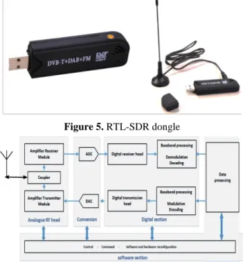
The receiver reconstructs the message sent from the captured signal by the inverted processing operations done on transmission. Those processes can be performed using a single SDR hardware and MATLAB software. RTL-SDR (fig. 5) or Software Defined Radio is a radio communication system, wherein the traditional hardware components (e.g. mixers, filters, amplifiers, modulators/demodulators, detectors, etc.) are instead implemented by means of software on an embedded system [21]. RTL-SDR is capable of receiving any signal in its frequency range. This range varies depending on the type of device used. In this work, the used dongle has a frequency capability of approximately 25MHz-1750MHz.
Figure 5. RTL-SDR dongle
Figure 6. Synoptic diagram of SDR card
• A configurable analog RF head, consisting of filters, couplers, mixers, intermediate frequency local oscillators, broadband and low noise power amplifiers,
• An analog / digital (ADC) and digital / analogue (DAC) conversion stage,
• A programmable digital section for shaping the spectrum, adapting and digital baseband processing, • Software section providing control and software
configuration of the various stages.
3.
The Energy Detection
3.1. Energy detection Model
The problem of spectrum sensing operation can be mathematically formulated as follows:
{𝑦(𝑡) = 𝑛(𝑡) ∶ 𝐻0
𝑦(𝑡) = 𝜀 ∗ 𝑥(𝑡) + 𝑛(𝑡) ∶ 𝐻1 Where 0 < 𝜀 ≤ 1 (1) Where:
𝑦(𝑡) : The received signal.
𝑥(𝑡)
: The signal to be detected, deterministic or random,
but unknown.𝑛(𝑡)
: The presented noise in the channel.
H0 is the hypothesis that the PU is not transmitting, therefore 𝑥(𝑡) = 0, while H1 is the hypothesis that the PU is using the channel for transmission. In the energy detection technique, we receive the signal 𝑦(𝑡), next we measure its energy by (2). The detection of the primary signal is done by comparing the measured energy with a threshold 𝜆 that presents the noise energy.
𝐸 =1
𝑇∑ [𝑌(𝑛)] 2 𝑁
𝑛=1 {
𝐸 > 𝜆 𝐻1 𝐸 < 𝜆 𝐻0
(2)
3.2. Energy detector implementation
The energy detection implementation is presented in Fig. 7. First, the received signal y (t), by RTL SDR dongle, is digitized by an analog to digital convertor (ADC) then passes through a band-pass filter (BPF), with a center frequency f0 and bandwidth W, using the transfer function (3) to select the desired band.
𝐻(𝑓) = {
2√𝑁0
|𝑓 − 𝑓
0| ≤ 𝑊
0 |𝑓 − 𝑓
0| > 𝑊
(3)
Then the filtered signal is transformed into frequency domain through the fast Fourier transform (FFT) block, and the signal energy is measured using (4).
𝐸 =1
𝑁∑ |𝑌(𝑓𝑖)| 2 𝑁
𝑖=1 (4) Finally, the estimated energy E is compared with a threshold λ (the noise energy) to decide if a signal is present (𝐻1) or not (𝐻0).
Figure 7. Block diagram of a frequency domain energy detector
4.
Artificial Neural Networks
4.1. The biological neuron
The biological neuron is a special biological cell that processes information. According to [22], there are huge number of neurons in the human brain, approximately 1011, each neuron is connected to 103 up to 104 other neurons. In total, approximately 1014 to 1015 interconnections. As shown in the fig. 8, a typical neuron mainly consists of the following three parts:
− The dendrites, which are the inputs of the neuron, collect the electrical information from the nervous system. − The soma that processes this information and sends back
an electrical signal of impulse type.
− The axon through which the outgoing signal is transmitted to neighboring neurons.
Figure 8. The biological neuron
4.2. The formal neuron
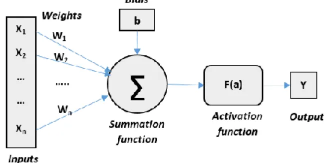
A formal neuron (fig. 9) is a mathematical function; it is conceived as a model of biological neuron. Formal neurons are elementary units in an artificial neural network. The following diagram represents the general mathematical model of a formal neuron [23]:
Figure 9. Mathematical model of the formal neuron The formal neuron that is given in the figure above has n inputs denoted as {𝑋1, 𝑋2, … , 𝑋𝑛}. Each line that connects these inputs to the summation junction is assigned a weight denoted as {𝑊1, 𝑊2, … , 𝑊𝑛}. The net input 𝑦𝑖𝑛can be calculated as follows:
International Journal of Communication Networks and Information Security (IJCNIS) Vol. 11, No. 1, April 2019
𝑦 = 𝐹(𝑦𝑖𝑛) = 𝐹 (∑ 𝑊𝑖∗ 𝑋𝑖+ 𝑏) (6)
Figure 10. sigmoid function
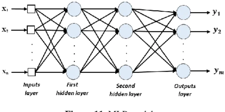
4.3. Multi-Layer Perceptron
The multilayer perceptron (MLP) (fig. 11) is a class of feedforward artificial neural network that has at least three layers of nodes. It generates a set of outputs {𝑦1, 𝑦2, … , 𝑦𝑚} from a set of inputs {𝑋1, 𝑋2, … , 𝑋𝑛}. Except for the input nodes, each node is a neuron that uses a nonlinear activation function.
Figure 11. MLP model
A neural network is trained with input and target pair patterns with the ability of learning. MLP can separate data that is not linearly distinguishable [24]. It is especially trained using a supervised learning technique called back-propagation (PB) algorithm [25], which aims at minimizing the global error measured at the output layer by the relation bellow:
𝑒(𝑡) = 𝑦𝑑(𝑡) − 𝑦𝑚(𝑡) (7) Where 𝑦𝑑(𝑡) denotes the desired output, and 𝑦𝑚(𝑡) the measured output of the neuron.
The BP algorithm uses an iterative supervised learning procedure, where the MLP is trained with a set of predefined inputs and outputs. The global error 𝐸𝑔(𝑡) is calculated by equation (8), this error can be minimized by the gradient descent technique [22].
𝐸𝑔(𝑡) =1
2∑ (𝑦𝑑,𝑖(𝑡) − 𝑦𝑚,𝑖(𝑡)) 2 𝑛
𝑖=1 (8)
There are several training algorithms that can be used to train an MLP network. In this paper, we will present a qualitative comparison between two training algorithms: quasi newton and conjugate gradient. Wherein the used training functions are respectively: trainlm (Levenberg Marquardt (LM)) and trainscg (Scaled Conjugate Gradient (SCG)). All these algorithms are trained by the same data set acquired from the implementation described in section II.
4.4. ANN implementation
We have proposed an ANN detector for spectrum sensing (Fig. 12), the ANN detector architecture is similar at the ED detector (Fig. 7), where the energy calculation block is replaced by an ANN block (Fig. 13).
Figure 12. ANN detection diagram
The number of input layer neurons n, is fixed by the points number (features) in the captured signal FFT vector. which is 1024 and we use one (1) neuron in the output layer (𝐻1 or 𝐻0):
Figure 13. The ANN architecture
5.
Support vector machines
Support vector machines (SVMs) are a new discriminating techniques in the theory of statistical learning, introduced in 1995s by V. Vapnik in his book " The Nature of Statistical Learning Theory "[26]. SVMs are machine learning methods that can be used to separate two classes of data [27, 28] by finding an optimal hyperplane ‘𝐻0’. This technique is essentially used for binary classification, but possible to classify samples with multiple classes. In addition, it can be used to solve both linear and nonlinear classification or regression problems. In SVMs, each input instance 𝑥, is represented by a pair (𝑥𝑖, 𝑦𝑖), where 𝑥𝑖 ∈ ℝ𝑛 is the data instance, and 𝑦𝑖∈ {1, −1} is the binary class label (positive or negative). The training data can be defined as:
𝐷 = {(𝑥𝑖, 𝑦𝑖) ∈ ℜ𝑛 , 𝑖 = 1, … , 𝑚 } (9)
The hyperplane ‘H’ can be defined by equation (10). Where the vector ‘𝜔’ is the weighing vector that defines the boundary of different classes of data, and ‘𝑏’ is a scalar threshold.
𝐻 ∶ (𝜔 . 𝑥) + 𝑏 (10)
The objective of SVM classification is to predict the value of 𝑦𝑖 for new data points 𝑥𝑖. There are two types in SVM classification: Linearly and non-linearly separable classification.
5.1. Linearly separable classification:
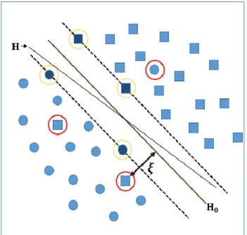
In this section, we present the general method of constructing the optimal hyperplane (OH), which separates data belonging to two different linearly separable classes. Fig. 14 gives a visual representation of the OH (𝐻0) in the case of linearly separable data, which is satisfying in the following conditions:
{𝜔 ∗ 𝑥𝑖+ 𝑏 ≥ 1 𝑖𝑓 𝑦𝑖= 1
𝜔 ∗ 𝑥𝑖+ 𝑏 ≤ −1 𝑖𝑓 𝑦𝑖= −1 (11)
That is equivalent to the next representation:
Figure 14. Separator hyperplanes: H is any hyperplane, Ho is the optimal hyperplane and M is the margin that represents the distance between the different classes and Ho (SV are the
Supports Vectors)
The optimal hyperplane 𝐻0 is a hyperplane that maximizes the margin M, which represents the smallest distance between the different data of the two classes and 𝐻0. Maximizing the margin M is equal to maximizing the sum of the distances between the two classes relative to 𝐻0. The margin ‘M’ has the following mathematical expression:
𝑀 = 𝑚𝑖𝑛
𝑥𝑖|𝑦𝑖=1𝜔∙𝑥+𝑏
‖𝜔‖
− 𝑚𝑎𝑥
𝑥𝑖|𝑦𝑖=−1 𝜔∙𝑥+𝑏‖𝜔‖
(13)
= 1 ‖𝜔‖−
−1
‖𝜔‖
𝑀
= 2‖𝜔‖ (14)
The optimal hyper plane can be obtained by maximizing the equation (14). Which is equivalent to minimizing (15):
min 𝜔
‖𝜔‖2
2 (15) The Equation (15) can be solved as a quadratic optimization problem by Lagrangian function:
𝐿(𝜔, 𝑏, 𝛼) =1 2‖𝜔‖
2− ∑ 𝛼𝑖 𝑚
𝑖=1
[𝑦𝑖(𝜔 ∙ 𝑥𝑖+ 𝑏) − 1] (16)
Where 𝛼𝑖= (𝛼1, … , 𝛼𝑚) > 0 is a lagrangian multiplier factors.
By deriving the equation (16) we obtain: 𝜔 = ∑ 𝛼𝑖
𝑚
𝑖=1
𝑦𝑖𝑥𝑖 (17)
∑ 𝛼𝑖 𝑚
𝑖=1
𝑦𝑖= 0 (18)
Substituting (17) and (18) into Equation (16), the optimal separating hyperplane can be obtained by solving the following dual representation of the optimization problem:
min 𝛼
1
2 ∑ 𝑦𝑖𝑦𝑗( 𝑚
𝑖,𝑗=1
𝑥𝑖𝑥𝑗)𝛼𝑖𝛼𝑗− ∑ 𝛼𝑗 (19) 𝑚
𝑗=1
Subject to ∑𝑚𝑖=1𝛼𝑖𝑦𝑖= 0 , 𝛼𝑖> 0
By solving this dual Lagrange function (19), 𝛼 is evaluated. Consequently, 𝜔 is evaluated out from (17), and 𝑏 can be easily calculated from (20):
𝑏 = 𝑦𝑗− ∑ 𝛼𝑖𝑦𝑖( 𝑚
𝑖=1
𝑥𝑖𝑥𝑗) (20)
Knowing that the classification function is defined by (21), where 𝑠𝑔𝑛 is a Signum function.
𝑐𝑙𝑎𝑠𝑠(𝑥) = 𝑠𝑔𝑛(𝜔 ∙ 𝑥𝑖+ 𝑏) (21)
Finally, we can classify an unknown data x by utilizing the following function:
𝑐𝑙𝑎𝑠𝑠(𝑥) = 𝑠𝑔𝑛 [∑ 𝛼𝑖𝑦𝑖( 𝑚
𝑖=1
𝑥𝑖𝑥) + 𝑏] (22)
5.2. Non-linearly separable classification:
If the classes of data are mixed (not linearly) (fig. 15), it is impossible to linearly separate the training data in the original space. In order to solve this non- linearly separable problem, the slack variables 𝜉𝑖, which cause little change around training data, are introduced. Then the training vectors must satisfy:
𝑦𝑖(𝜔 ∙ 𝑥𝑖+ 𝑏) ≥ 1 − 𝜉𝑖 , 𝑖 = 1, … … , 𝑚 (23)
In the case when the data points are not linearly separable in the data space, the SVM handles this by using a kernel function to map the data to a transformed feature space (a higher dimensional space) where a hyperplane is then used to gain linearly separation. For this, we project the original data into the feature space using non-linear functions. In this new space we build the OH that separates the transformed data. The main problem here is how to manipulate the transformation of all input vectors in the feature space, so as to avoid an increase in the cost in number of free parameters. Let the set 𝐷′be the image (the transformed feature space) of the set D defined in previous section, by the transformation: 𝐷′= {𝜓(𝑥𝑖), 𝑦𝑖) ∈ ℜ𝑛× {−1,1}, 𝑖 = 1, … , 𝑚| 𝑝 ≥ 𝑛 } (24)
Structuring an optimal hyperplane, defined by the weight vector 𝜔 and the bias b is solved as a quadratic optimization problem that maximizes the margin between the classes (The first part of Eq. 25), and minimizes the errors (The second part of Eq. 25). It can be expressed as:
𝑚𝑖𝑛 [1 2‖𝜔‖
2+ 𝐶 ∑ 𝜉 𝑖 𝑚
𝑖=1
] (25)
Subject to { 𝑦𝑖(𝜔 ∙ 𝑥𝑖+ 𝑏) ≥ 1 − 𝜉𝑖 𝜉𝑖≥ 0 ; 𝑖 = 1, … … , 𝑚
International Journal of Communication Networks and Information Security (IJCNIS) Vol. 11, No. 1, April 2019
Figure 15. Separator hyperplanes in the case of non-linearly separable (𝜉 is the slack variables)
Using Lagrange multiplier technique, the above optimization problem (25) can be reformulated as:
𝐿(𝜔, 𝑏, 𝜉, 𝛼, 𝛽) =1 2‖𝜔‖
2+ 𝐶 ∑ 𝜉𝑖 𝑚
𝑖=1
− ∑ 𝛽𝑖𝜉𝑖 𝑚
𝑖=1
− ∑ 𝛼𝑖 𝑚
𝑖=1
[𝑦𝑖(𝜔𝑇𝜓(𝑥𝑖) + 𝑏) − 1
+ 𝜉𝑖] (26)
Where 𝛼𝑖 and β𝑖 are positive Lagrangian multipliers parameters that can be found by solving the quadratic programming problem (26). The obtained vector 𝛼 is known as a support vector. By applying Karush-Kuhn-Tucker (KKT) conditions, which is a theorem that plays an important part in the theory of optimization, to (26), we can obtain:
𝜔 = ∑ 𝛼𝑖𝑦𝑖𝜓(𝑥𝑖) (27) 𝑚
𝑖=1
∑ 𝛼𝑖𝑦𝑖= 0 𝑚
𝑖=1
(28)
𝛼𝑖= 𝐶 − 𝛽𝑖 (29)
It is noticeable that 0 ≤ 𝛼𝑖≤ 𝐶 and 𝛽𝑖≥ 0.
By calculating the derivatives with respect to 𝜔, 𝑏 and 𝜉, the dual representation of the optimization problem in term of support vectors can be obtained as follows [28].
max ∑ 𝛼𝑖−1 2 𝑚
𝑖=1
∑ 𝛼𝑖𝛼𝑗 𝑚
𝑖,𝑗=1
𝑦𝑖𝑦𝑗𝐾(𝑥𝑖, 𝑥𝑗) (30)
Subject to
{ ∑ 𝛼𝑖
𝑚
𝑖=1 𝑦𝑖= 0
0 ≤ 𝛼𝑖≤ 𝐶 ; 𝑖 = 1, … … , 𝑚 (31)
Where 𝐾(𝑥𝑖, 𝑥𝑗) = 𝜓(𝑥𝑖)𝜓(𝑥𝑗) is the kernel function. Hence, by solving the optimization function defined in (30), the resulting nonlinear classification function can be obtained as follows:
𝑐𝑙𝑎𝑠𝑠(𝑥) = 𝑠𝑔𝑛 [ ∑ 𝛼𝑖 𝑥𝑖∈ 𝑉𝑆
𝑦𝑖𝐾(𝑥𝑖, 𝑥) + 𝑏 ] (32)
𝜓(𝑥𝑗) The most common kernel, that are widely used because of their efficiency in mapping the input data to higher dimensional space in order to reduce the computational load, are illustrated as follows (𝑢 and 𝑣 are vectors) [28].
− The linear kernel:
𝐾(𝑢, 𝑣) = 𝑢. 𝑣 (33) − The Polynomial kernel:
𝐾(𝑢, 𝑣) = [(𝑢. 𝑣) + 1]𝑑 (34) − The RBF kernel (Radial Basis Function): 𝐾(𝑢, 𝑣) = 𝑒𝑥𝑝(−‖𝑢 − 𝑣‖
2
2𝜎2 ) (35)
5.3. SVM implementation:
Support Vector Machine (SVM) model is a powerful supervised machine learning, it is used for efficient classification with high precision in various applications like object detection, speech recognition, bioinformatics, image classification, medical diagnosis and others [29]. In our context, we have proposed an SVM detector diagram for signal classification (spectrum sensing) (Fig. 16). Our SVM detector have the same steps of the ANN detector (fig. 12), we have just changed the ANN block by an SVM block.
Figure 16. SVM detection diagram
The SVM kernel choice is critical to define the flexibility and classification power. The most used kernels are: linear, polynomial degree ‘p’, and Gaussian. In MATLAB software, we can find three principle SVM functions for classification [30]: “fitcsvm”, “fitclinear” and “fitckernel”.
− The Fitcsvm function (fit a classifier using SVM), trains a support vector machine (SVM) model for binary classification (two classes), on a low-dimensional or moderate-dimensional predictor data set.
− The fitclinear (Fit linear classification) function trains linear classification models for two-class (binary) learning with high-dimensional. This function minimizes the objective function using techniques that reduce computing time (e.g., stochastic gradient descent).
− The fitckernel (fit classifier kernel) function trains a binary Gaussian kernel classification model for nonlinear classification. it is more practical for big data applications that have large training sets, but can also be applied to smaller data sets. This function maps data in a higher dimensional space then fits a linear model in the new space by minimizing the regularized objective function.
6.
Implementation and Results
The collected database contains 1600 signals with ASK and FSK modulation type. The proposed work is implemented in MATLAB 9.4.0 (R2018a) for a 64-bit computer with core i3 processor, clock speed 2.4 GHz, and 6 GB RAM.
Table 1 is showing how we have used our database in the learning phase and test phase:
Table 1.Data-base used in learning and testing
Signal Learning phase Test phase
Primary signal 600 300
Noise 400 300
Figure 17. Chart of the energy detection operation
The performance of an energy detector can be characterized using two probabilities: 𝑃𝑑 the probability of detection and 𝑃𝑓𝑎 the false alarm probability.
𝑃𝑑 : The probability of detecting a signal in the band of interest, when this signal is truly present (𝐻1). Failed detection causes interference with the PU. We calculated 𝑃𝑑 by (36):
𝑃𝑑 = 𝑃 (𝑑𝑒𝑐𝑖𝑠𝑖𝑜𝑛 𝐻1/𝐻1) = 𝑁𝑐
𝑁 × 100 (36) 𝑃𝑓𝑎 : The probability when the test falsely decides that the band of interest is occupied, while it is free (𝐻0). The False alarm reduces the efficiency of spectrum use. We calculated 𝑃𝑓𝑎 by (37):
𝑃𝑓𝑎 = 𝑃 (𝑑𝑒𝑐𝑖𝑠𝑖𝑜𝑛 𝐻1/𝐻0) = 𝑁𝑒
𝑁 × 100 (37) Where:
𝑁𝑐: The number of times in which the signal is detected, while 𝐻1;
𝑁𝑒 : The number of times in which the signal is detected, while 𝐻0;
𝑁 : The number of the captured signals. 6.1. Energy Detection results:
The detection of the transmitted signal, using the energy detection method, is done in MATLAB software according to the flowchart of Fig. 17. We have as an input a frequency vector that contains ‘N’ signals data, which is captured by the RTL-SDR.
Following this flowchart, we calculate the probability of detection 𝑃𝑑 . While we calculate the false alarm probability 𝑃𝑓𝑎 by stopping the emission operation and following the same previous steps using (37) instead of (36). The values of 𝑷𝒅 and 𝑷𝒇𝒂 obtained through the energy detector (fig. 7) are shown in the table 2:
Table 2.The probability of detection and the false alarm probability of ED
𝑷𝒅 𝑷𝒇𝒂
0.99 0,015
6.2. Artificial neural network results
International Journal of Communication Networks and Information Security (IJCNIS) Vol. 11, No. 1, April 2019 Table 3.Probability of detection and the false alarm
probability in testing phase for ANN detector
Number of neurons in the
hidden layer
Training
function 𝑷𝒅 𝑷𝒇𝒂
3
SCG 0.983 0.017
LM 0.963 0.020
4
SCG 0.973 0.013
LM 0.966 0.043
5
SCG 0.980 0.0167
LM 0.960 0.046
6
SCG 0.970 0.0167
LM 0.973 0.0167
7
SCG 0.963 0.0267
LM 0.960 0.023
8
SCG 0.970 0.0131
LM 0.983 0.007
10
SCG 0.970 0.0233
LM 0.956 0.0267
The results show that the best performance is obtained for the training function ‘trainlm’ with 8 hidden neurons, in which the probabilities 𝑷𝒅 and 𝑷𝒇𝒂 are presented in the following table.
Table 4.The probability of detection and the false alarm probability of ANN detection
𝑷𝒅 𝑷𝒇𝒂
0.983 0.007
6.3. Support vector machines results
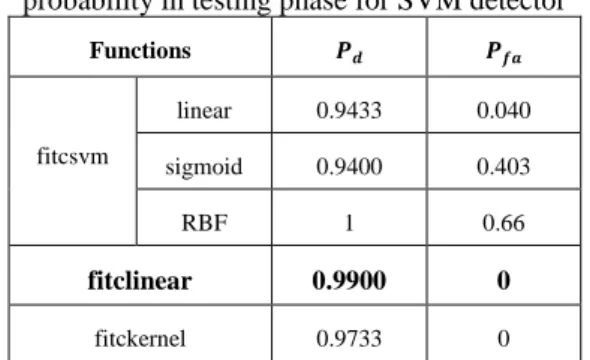
The SVM training phase builds a model for classifying any future data based on the Support Vectors (SVs) identified from a training dataset. The SVs are then used in the classification phase to predict the appropriate class of an input test data. In order to determine the most convenient SVM function for our SVM detector, we have compared the performance of the above three functions. The implementation results of the SVM detector (fig. 16) are presented in table 5, the following table shows the comparison of classification performance for the three SVM functions.
Table 5.Probability of detection and the false alarm probability in testing phase for SVM detector
Functions 𝑷𝒅 𝑷𝒇𝒂
fitcsvm
linear 0.9433 0.040
sigmoid 0.9400 0.403
RBF 1 0.66
fitclinear 0.9900 0
fitckernel 0.9733 0
From this table we can see that the function “fitclinear” has shown high classification accuracy rates outperforming the other functions.
6.4. Discussion
Energy detection has the advantages of low complexity, ease of implementation, and extensive use of properties without knowing the signal. However, when there is a low signal noise ratio (SNR), there are many problems that decrease the performance of energy detection method, and make it hard to set the threshold. In the classic method, we use a static threshold, but as we know, the threshold depends on the environmental noise. Whereas the ANN detector and the SVM detector, give the best results and they have a stable performance in comparison with the classical energy detection method. The excellent results have been reported in applying SVM’s in spectrum sensing.
7.
Conclusions
References
[1] Federal Communications Commission, Spectrum Policy Task Force, “Report of the Spectrum Efficiency Working Group,” November 2002.
[2] P. Kolodzy, "Next generation communications: Kickoff meeting," in Proc. DARPA, vol. 10, 2001.
[3] J. Mitola G. Q. Maguire, "Cognitive radio: making software radios more personal," IEEE personal communications, vol. 6, No. 4, pp. 13-18, 1999.
[4] J. Mitola Iii, "Cognitive radio for flexible mobile multimedia communications," Mobile Networks and Applications, vol. 6, No. 5, pp. 435-441, 2001.
[5] S. Haykin, "Cognitive radio: brain-empowered wireless communications," IEEE journal on selected areas in communications, vol. 23, No. 2, pp. 201-220, 2005.
[6] T. Yucek H. Arslan, "A survey of spectrum sensing algorithms for cognitive radio applications," IEEE communications surveys & tutorials, vol. 11, No. 1, pp. 116-130, 2009. [7] D. Cabric, S. M. Mishra, R. W. Brodersen, "Implementation
issues in spectrum sensing for cognitive radios," in Signals, systems and computers, 2004. Conference record of the thirty-eighth Asilomar conference on, vol. 1, pp. 772-776, 2004. [8] W. Ejaz, ul Hasan, N., Lee, S. et al. , "Intelligent spectrum
sensing scheme for cognitive radio networks," EURASIP Journal on Wireless Communications and Networking, vol. 1, pp. 1-10, 2013.
[9] F. F. Digham, M.-S. Alouini, M. K. Simon, "On the energy detection of unknown signals over fading channels," IEEE International Conference on Communications, Anchorage, AK, USA, vol. 5, pp. 3575-3579, 2003.
[10] V. I. Kostylev, "Energy detection of a signal with random amplitude," IEEE International Conference on Communications, New York, USA, vol. 3, pp. 1606-1610, 2002.
[11] K. Kim, I. A. Akbar, K. K. Bae, J.-S. Um, C. M. Spooner, J. H. Reed, "Cyclostationary approaches to signal detection and classification in cognitive radio," 2nd IEEE International Symposium on New Frontiers in Dynamic Spectrum Access Networks, Dublin, Ireland, pp. 212-215, 2007.
[12] Sai Shankar N, C. Cordeiro and K. Challapali, "Spectrum agile radios: utilization and sensing architectures," First IEEE International Symposium on New Frontiers in Dynamic Spectrum Access Networks, Baltimore, MD, USA, pp. 160-169, 2005.
[13] S. Atapattu, C. Tellambura, H. Jiang, "Energy detection based cooperative spectrum sensing in cognitive radio networks," IEEE Transactions on wireless communications, vol. 10, No. 4, pp. 1232-1241, 2011.
[14] S. Ali, K. A. Smith, "On learning algorithm selection for classification," Applied Soft Computing, vol. 6, No. 2, pp. 119-138, 2006.
[15] K. M. Thilina, K. W. Choi, N. Saquib, E. Hossain, "Machine learning techniques for cooperative spectrum sensing in cognitive radio networks," IEEE Journal on selected areas in communications, vol. 31, No. 11, pp. 2209-2221, 2013. [16] I. Guyon, J. Weston, S. Barnhill, V. Vapnik, "Gene selection
for cancer classification using support vector machines," Machine learning, vol. 46, No. 1-3, pp. 389-422, 2002. [17] P. Singh, V. Pareek, A. K. Ahlawat, "Designing an Energy
Efficient Network Using Integration of KSOM, ANN and Data Fusion Techniques," International Journal of Communication Networks and Information Security (IJCNIS), vol. 9, No. 3, 2017.
[18] B. Benmammar, Y. Benmouna, A. Amraoui, F. Krief, "A parallel implementation on a multi-core architecture of a dynamic programming algorithm applied in cognitive radio ad hoc networks," International Journal of Communication Networks and Information Security (IJCNIS), vol. 9, No. 2, 2017.
[19] A. Elrharras, R. Saadane, M. Wahbi, A. Hamdoun, "Neural Networks and PCA for Spectrum Sensing in the context of Cognitive Radio," Proceedings of the Mediterranean Conference on Information & Communication Technologies, pp. 173-181, 2016.
[20] A. Elrharras, R. Saadane, M. Wahbi, A. Hamdoun, "Signal detection and automatic modulation classification based spectrum sensing using PCA-ANN with real word signals," Applied Mathematical Sciences, vol. 8, No. 160, pp. 7959-7977, 2014.
[21] M. Dillinger, K. Madani, N. Alonistioti, Software defined radio: Architectures, systems and functions. John Wiley & Sons, 2005.
[22] A. K. Jain, J. Mao, K. M. Mohiuddin, "Artificial neural networks: A tutorial," Computer, vol. 29, No. 3, pp. 31-44, 1996.
[23] M. T. Hagan, H. B. Demuth, M. H. Beale,"Neural network design," Boston, 1996.
[24] G. Cybenko, "Approximation by superpositions of a sigmoidal function," Mathematics of control, signals and systems, vol. 2, No. 4, pp. 303-314, 1989.
[25] K. Tsagkaris, A. Katidiotis, P. Demestichas, "Neural network-based learning schemes for cognitive radio systems," Computer Communications, vol. 31, No. 14, pp. 3394-3404, 2008.
[26] V. Vapnik, The nature of statistical learning theory. Springer science & business media, 2013.
[27] C. J. Burges, "A tutorial on support vector machines for pattern recognition," Data mining and knowledge discovery, vol. 2, No. 2, pp. 121-167, 1998.
[28] C. Cortes V. Vapnik, "Support-vector networks," Machine learning, vol. 20, No. 3, pp. 273-297, 1995.
[29] J. Nayak, B. Naik, H. Behera, "A comprehensive survey on support vector machine in data mining tasks: applications & challenges," International Journal of Database Theory and Application, vol. 8, No. 1, pp. 169-186, 2015.