Applied Spatial Data Analysis with R - Free Computer, Programming, Mathematics, Technical Books, Lecture Notes and Tutorials

(1)

Series Editors:

(2)

Use R!

Albert:Bayesian Computation with R

Bivand/Pebesma/Gómez-Rubio:Applied Spatial Data Analysis with R Cook/Swayne:Interactive and Dynamic Graphics for Data Analysis:

With R and GGobi

Hahne/Huber/Gentleman/Falcon:Bioconductor Case Studies Paradis:Analysis of Phylogenetics and Evolution with R

Pfaff:Analysis of Integrated and Cointegrated Time Series with R Sarkar:Lattice: Multivariate Data Visualization with R

(3)

Roger S. Bivand

Edzer J. Pebesma

Virgilio Gómez-Rubio

Applied Spatial Data

Analysis with R

(4)

Norwegian School of Economics and Business Administration Breiviksveien 40

5045 Bergen Norway

Edzer J. Pebesma University of Utrecht

Department of Physical Geography 3508 TC Utrecht

Netherlands

Department of Epidemiology and Public Health

Imperial College London St. Mary’s Campus Norfolk Place London W2 1PG United Kingdom

Series Editors: Robert Gentleman

Program in Computational Biology Division of Public Health Sciences Fred Hutchinson Cancer Research Center 1100 Fairview Ave. N, M2-B876 Seattle, Washington 98109-1024 USA

Giovanni Parmigiani

The Sidney Kimmel Comprehensive Cancer Center at Johns Hopkins University 550 North Broadway

Baltimore, MD 21205-2011 USA

Kurt Hornik

Department für Statistik und Mathematik Wirtschaftsuniversität Wien Augasse 2-6 A-1090 Wien

Austria

ISBN 978-0-387-78170-9 e-ISBN 978-0-387-78171-6 DOI 10.1007/978-0-387-78171-6

Library of Congress Control Number: 2008931196 c

2008 Springer Science+Business Media, LLC

All rights reserved. This work may not be translated or copied in whole or in part without the written permission of the publisher (Springer Science+Business Media, LLC, 233 Spring Street, New York, NY 10013, USA), except for brief excerpts in connection with reviews or scholarly analysis. Use in connection with any form of information storage and retrieval, electronic adaptation, computer software, or by similar or dissimilar methodology now known or hereafter developed is forbidden.

The use in this publication of trade names, trademarks, service marks, and similar terms, even if they are not identiﬁed as such, is not to be taken as an expression of opinion as to whether or not they are subject to proprietary rights.

(5)

Voor Ellen, Ulla en Mandus

(6)

Preface

We began writing this book in parallel with developing software for handling and analysing spatial data with R (R Development Core Team, 2008). Al-though the book is now complete, software development will continue, in the

Rcommunity fashion, of rich and satisfying interaction with users around the world, of rapid releases to resolve problems, and of the usual joys and frustra-tions of getting things done. There is little doubt that without pressure from users, the development of Rwould not have reached its present scale, and the same applies to analysing spatial data analysis withR.

It would, however, not be suﬃcient to describe the development of the

Rproject mainly in terms of narrowly deﬁned utility. In addition to being a community project concerned with the development of world-class data analy-sis software implementations, it promotes speciﬁc choices with regard to how data analysis is carried out. R is open source not only because open source software development, including the dynamics of broad and inclusive user and developer communities, is arguably an attractive and successful development model.

Ris also, or perhaps chieﬂy, open source because the analysis of empirical and simulated data in science should be reproducible. As working researchers, we are all too aware of the possibility of reaching inappropriate conclusions in good faith because of user error or misjudgement. When the results of research really matter, as in public health, in climate change, and in many other ﬁelds involving spatial data, good research practice dictates that some-one else should be, at least in principle, able to check the results. Open source software means that the methods used can, if required, be audited, and jour-nalling working sessions can ensure that we have a record of what we actually did, not what we thought we did. Further, usingSweave1– a tool that permits the embedding of Rcode for complete data analyses in documents – through-out this book has provided crucial support (Leisch, 2002; Leisch and Rossini, 2003).

(7)

We acknowledge our debt to the members of R-core for their continu-ing commitment to the Rproject. In particular, the leadership and example of Professor Brian Ripley has been important to us, although our admitted ‘muddling through’ contrasts with his peerless attention to detail. His inter-ested support at the Distributed Statistical Computing conference in Vienna in 2003 helped us to see that encouraging spatial data analysis in R was a project worth pursuing. Kurt Hornik’s dedication to keep the Comprehensive

R Archive Network running smoothly, providing package maintainers with superb, almost 24/7, service, and his dry humour when we blunder, have meant that the useRcommunity is provided with contributed software in an unequalled fashion. We are also grateful to Martin M¨achler for his help in setting up and hosting the R-Sig-Geo mailing list, without which we would have not had a channel for fostering theRspatial community.

We also owe a great debt to users participating in discussions on the mail-ing list, sometimes for speciﬁc suggestions, often for fruitful questions, and occasionally for perceptive bug reports or contributions. Other users contact us directly, again with valuable input that leads both to a better understanding on our part of their research realities and to the improvement of the software involved. Finally, participants at Rspatial courses, workshops, and tutorials have been patient and constructive.

We are also indebted to colleagues who have contributed to improving the final manuscript by commenting on earlier drafts and pointing out better pro-cedures to follow in some examples. In particular, we would like to mention Juanjo Abellán, Nicky Best, Peter J. Diggle, Paul Hiemstra, Rebeca Ramis, Paulo J. Ribeiro Jr., Barry Rowlingson, and Jon O. Skøien. We are also grate-ful to colleagues for agreeing to our use of their data sets. Support from Luc Anselin has been important over a long period, including a very fruitful CSISS workshop in Santa Barbara in 2002. Work by colleagues, such as the first book known to us on usingRfor spatial data analysis (Kopczewska, 2006), provided further incentives both to simplify the software and complete its description. Without John Kimmel’s patient encouragement, it is unlikely that we would have finished this book.

Even though we have beneﬁtted from the help and advice of so many people, there are bound to be things we have not yet grasped – so remaining mistakes and omissions remain our sole responsibility. We would be grateful for messages pointing out errors in this book; errata will be posted on the book website (http://www.asdar-book.org).

Bergen Roger S. Bivand

M¨unster Edzer J. Pebesma

London Virgilio G´omez-Rubio

(8)

Part I

(15)

The key intuition underlying the development of the classes and methods in thesp package, and its closer dependent packages, is that users approaching

R with experience of GIS will want to see ‘layers’, ‘coverages’, ‘rasters’, or ‘geometries’. Seen from this point of view, sp classes should be reasonably familiar, appearing to be well-known data models. On the other hand, for sta-tistician users of R, ‘everything’ is adata.frame, a rectangular table with rows of observations on columns of variables. To permit the two disparate groups of users to play together happily, classes have grown that look like GIS data models to GIS and other spatial data people, and look and behave like data frames from the point of view of applied statisticians and other data analysts. This part of the book describes the classes and methods of thesppackage, and in doing so also provides a practical guide to the internal structure of many GIS data models, asRpermits the user to get as close as desired to the data. However, users will not often need to know more than that of Chap. 4 to read in their data and start work. Visualisation is covered in Chap. 3, and so a statistician receiving a well-organised set of data from a collaborator may even be able to start making maps in two lines of code, one to read the data and one to plot the variable of interest using lattice graphics. Note that coloured versions of ﬁgures may be found on the book website together with complete code examples, data sets, and other support material.

(16)

1 Hello World

: Introducing Spatial Data

1.1 Applied Spatial Data Analysis

Spatial dataare everywhere. Besides those we collect ourselves (‘is it raining?’),

they confront us on television, in newspapers, on route planners, on computer screens, and on plain paper maps. Making a map that is suited to its purpose and does not distort the underlying data unnecessarily is not easy. Beyond creating and viewing maps, spatial data analysisis concerned with questions not directly answered by looking at the data themselves. These questions refer to hypothetical processes that generate the observed data. Statistical inference for such spatial processes is often challenging, but is necessary when we try to draw conclusions about questions that interest us.

Possible questions that may arise include the following:

• Does the spatial patterning of disease incidences give rise to the conclusion that they are clustered, and if so, are the clusters found related to factors such as age, relative poverty, or pollution sources?

• Given a number of observed soil samples, which part of a study area is polluted?

• Given scattered air quality measurements, how many people are exposed to high levels of black smoke or particulate matter (e.g. PM₁₀),1_{and where}

do they live?

• Do governments tend to compare their policies with those of their neigh-bours, or do they behave independently?

In this book we will be concerned withappliedspatial data analysis, meaning that we will deal with data sets, explain the problems they confront us with, and show how we can attempt to reach a conclusion. This book will refer to the theoretical background of methods and models for data analysis, but emphasise hands-on, do-it-yourself examples using R; readers needing this background should consult the references. All data sets used in this book and all examples given are available, and interested readers will be able to reproduce them.

(17)

In this chapter we discuss the following: (i) Why we useRfor analysing spatial data

(ii) The relation betweenRand geographical information systems (GIS) (iii) What spatial data are, and the types of spatial data we distinguish (iv) The challenges posed by their storage and display

(v) The analysis of observed spatial data in relation to processes thought to have generated them

(vi) Sources of information about the use of Rfor spatial data analysis and the structure of the book.

1.2 Why Do We Use

R

1.2.1 ... In General?

TheRsystem2 _{(R Development Core Team, 2008) is a free software}

environ-ment for statistical computing and graphics. It is an impleenviron-mentation of the S language for statistical computing and graphics (Becker et al., 1988). For data analysis, it can be highly eﬃcient to use a special-purpose language like S, compared to using a general-purpose language.

For new R users without earlier scripting or programming experience, meeting a programming language may be unsettling, but the investment3_will

quickly pay oﬀ. The user soon discovers how analysis components – written or copied from examples — can easily be stored, replayed, modiﬁed for another data set, or extended.R can be extended easily with new dedicated compo-nents, and can be used to develop and exchange data sets and data analysis approaches. It is often much harder to achieve this with programs that require long series of mouse clicks to operate.

Rprovides many standard and innovative statistical analysis methods. New users may ﬁnd access to both well-tried and trusted methods, and speculative and novel approaches, worrying. This can, however, be a major strength, be-cause if required, innovations can be tested in a robust environment against legacy techniques. Many methods for analysing spatial data are less frequently used than the most common statistical techniques, and thus beneﬁt pro-portionally more from the nearness to both the data and the methods that

Rpermits.Ruses well-known libraries for numerical analysis, and can easily be extended by or linked to code written inS, C, C++, Fortran, or Java. Links to various relational data base systems and geographical information systems exist, many well-known data formats can be read and/or written.

The level of voluntary support and the development speed of Rare high, and experience has shown Rto be environment suitable for developing pro-fessional, mission-critical software applications, both for the public and the

2_{http://www.r-project.org.}

(18)

private sector. TheSlanguage can not only be used for low-level computation on numbers, vectors, or matrices but can also be easily extended with classes for new data types and analysis methods for these classes, such as meth-ods for summarising, plotting, printing, performing tests, or model ﬁtting (Chambers, 1998).

In addition to the coreRsoftware system,Ris also a social movement, with many participants on a continuum from useRs just beginning to analyse data withRto developeRs contributing packages to the ComprehensiveRArchive Network4 _{(CRAN) for others to download and employ.}

Just as R itself beneﬁts from the open source development model, con-tributed package authors beneﬁt from a world-class infrastructure, allowing their work to be published and revised with improbable speed and reliability, including the publication of source packages and binary packages for many popular platforms. Contributed add-on packages are very much part of the

Rcommunity, and most core developers also write and maintain contributed packages. A contributed package contains Rfunctions, optional sample data sets, and documentation including examples of how to use the functions.

1.2.2 ... for Spatial Data Analysis?

For over 10 years,Rhas had an increasing number of contributed packages for handling and analysing spatial data. All these packages used to make differ-ent assumptions about how spatial data were organised, andRitself had no capabilities for distinguishing coordinates from other numbers. In addition, methods for plotting spatial data and other tasks were scattered, made differ-ent assumptions on the organisation of the data, and were rudimdiffer-entary. This was not unlike the situation for time series data at the time.

After some joint eﬀort and wider discussion, a group5 _of _R _developers

have written the R package sp to extend R with classes and methods for spatial data (Pebesma and Bivand, 2005). Classes specify a structure and deﬁne how spatial data are organised and stored. Methods are instances of functions specialised for a particular data class. For example, the summary method for all spatial data classes may tell the range spanned by the spatial coordinates, and show which coordinate reference system is used (such as degrees longitude/latitude, or the UTM zone). It may in addition show some more details for objects of a speciﬁc spatial class. A plot method may, for example create a map of the spatial data.

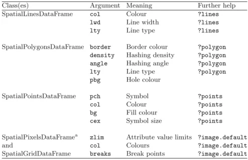
Thesp package provides classes and methods for points, lines, polygons, and grids (Sect. 1.4, Chap. 2). Adopting a single set of classes for spatial data oﬀers a number of important advantages:

4_{CRAN mirrors are linked from}_{http://www.r-project.org/.}

5_{Mostly the authors of this book with help from Barry Rowlingson and Paulo J.}

(19)

(i) It is much easier to move data across spatial statistics packages. The classes are either supported directly by the packages, reading and writing data in the new spatial classes, or indirectly, for example by supplying data conversion between the sp classes and the package’s classes in an interface package. This last option requires one-to-many links between the packages, which are easier to provide and maintain than many-to-many links.

(ii) The new classes come with a well-tested set of methods (functions) for plotting, printing, subsetting, and summarising spatial objects, or com-bining (overlaying) spatial data types.

(iii) Packages with interfaces to geographical information systems (GIS), for reading and writing GIS ﬁle formats, and for coordinate (re)projection code support the new classes.

(iv) The new methods include Lattice plots, conditioning plots, plot methods that combine points, lines, polygons, and grids with map elements (refer-ence grids, scale bars, north arrows), degree symbols (as in 52◦N) in axis labels, etc.

Chapter 2 introduces the classes and methods provided by sp, and discusses some of the implementation details. Further chapters will show the degree of integration of sp classes and methods and the packages used for statistical analysis of spatial data.

Figure 1.1 shows how the reception ofspclasses has already inﬂuenced the landscape of contributed packages; interfacing other packages for handling and analysing spatial data is usually simple as we see in Part II. The shaded nodes of the dependency graph are packages (co)-written and/or maintained by the authors of this book, and will be used extensively in the following chapters.

1.3 R

and GIS

1.3.1 What is GIS?

Storage and analysis of spatial data is traditionally done in Geographical Infor-mation Systems (GIS). According to the toolbox-based deﬁnition of Burrough and McDonnell (1998, p. 11), a GIS is ‘...a powerful set of tools for collecting, storing, retrieving at will, transforming, and displaying spatial data from the real world for a particular set of purposes’. Another deﬁnition mentioned in the same source refers to ‘...checking, manipulating, and analysing data, which are spatially referenced to the Earth’.

(20)

(21)

solved using an environment such asR, but whether it can be solvedeﬃciently

withR. In some cases, combining diﬀerent software components in a workﬂow may be the most robust solution, for example scripting in languages such as Python.

1.3.2 Service-Oriented Architectures

Today, much of the practice and research in geographical information sys-tems is moving from toolbox-centred architectures (think of the ‘classic’ Arc/Info™ or ArcGIS™ applications) towards service-centred architectures (such as Google Earth™). In toolbox-centred architectures, the GIS appli-cation and data are situated on the user’s computer or local area network. In service-centred architectures, the tools and data are situated on remote computers, typically accessed through Internet connections.

Reasons for this change are the increasing availability and bandwidth of the Internet, and also ownership and maintenance of data and/or analysis methods. For instance, data themselves may not be freely distributable, but certain derived products (such as visualisations or generalisations) may be. A service can be kept and maintained by the provider without end users having to bother about updating their installed software or data bases. TheRsystem operates well under both toolbox-centred and service-centred architectures.

1.3.3 Further Reading on GIS

It seems appropriate to give some recommendations for further reading con-cerning GIS, not least because a more systematic treatment would not be appropriate here. Chrisman (2002) gives a concise and conceptually elegant introduction to GIS, with weight on using the data stored in the system; the domain focus is on land planning. A slightly older text by Burrough and McDonnell (1998) remains thorough, comprehensive, and perhaps a shade closer to the earth sciences in domain terms than Chrisman.

Two newer comprehensive introductions to GIS cover much of the same ground, but are published in colour. Heywood et al. (2006) contains less extra material than Longley et al. (2005), but both provide very adequate coverage of GIS as it is seen from within the GIS community today. To supplement these, Wise (2002) provides a lot of very distilled experience on the technical-ities of handling geometries in computers in a compact form, often without dwelling on the computer science foundations; these foundations are given by Worboys and Duckham (2004). Neteler and Mitasova (2008) provide an ex-cellent analytical introduction to GIS in their book, which also shows how to use the open source GRASS GIS, and how it can be interfaced withR.

(22)

systems far more than the standard texts. Two hands-on alternatives show how service-centred architectures can be implemented at low cost by non-specialists, working, for example in environmental advocacy groups, or volun-teer search and rescue teams (Mitchell, 2005; Erle et al., 2005); their approach is certainly not academic, but gets the job done quickly and eﬀectively.

In books describing the handling of spatial data for data analysts (looking at GIS from the outside), Waller and Gotway (2004, pp. 38–67) cover most of the key topics, with a useful set of references to more detailed treatments; Banerjee et al. (2004, pp. 10–18) give a brief overview of cartography suﬃcient to get readers started in the right direction.

1.4 Types of Spatial Data

Spatial data have spatial reference: they have coordinate values and a system of reference for these coordinates. As a fairly simple example, consider the locations of volcano peaks on the Earth. We could list the coordinates for all known volcanoes as pairs of longitude/latitude decimal degree values with respect to the prime meridian at Greenwich and zero latitude at the equator. The World Geodetic System (WGS84) is a frequently used representation of the Earth.

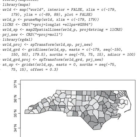
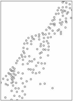
Suppose we are interested in the volcanoes that have shown activity be-tween 1980 and 2000, according to some agreed seismic registration system. This data set consists of points only. When we want to draw these points on a (ﬂat) map, we are faced with the problem of projection: we have to translate from the spherical longitude/latitude system to a new, non-spherical coor-dinate system, which inevitably changes their relative positions. In Fig. 1.2, these data are projected using a Mollweide projection, and, for reference pur-poses, coast lines have been added. Chapter 4 deals with coordinate reference systems, and with transformations between them.

0°

75°S 60°S 45°S 30°S 15°S

0°

15°N 30°N

45°N 60°N

75°N

(23)

If we also have the date and time of the last observed eruption at the volcano, this information is called an attribute: it is non-spatial in itself, but this attribute information is believed to exist for each spatial entity (volcano). Without explicit attributes, points usually carry implicit attributes, for example all points in this map have the constant implicit attribute – they mark a ‘volcano peak’, in contrast to other points that do not. We represent

the purely spatialinformation of entities by data models.The diﬀerent types

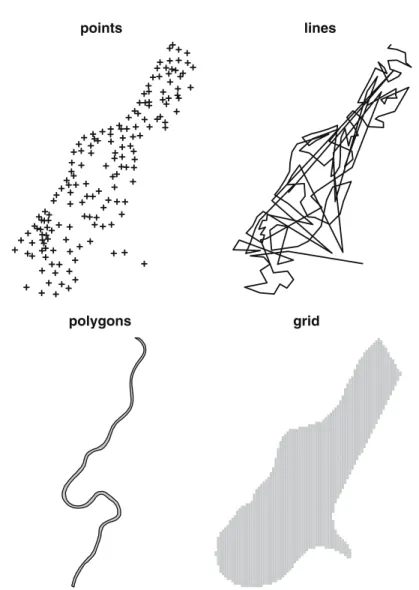
of data models that we distinguish here include the following:

Point, a single point location, such as a GPS reading or a geocoded address

Line, a set of ordered points, connected by straight line segments

Polygon, an area, marked by one or more enclosing lines, possibly containing

holes

Grid, a collection of points or rectangular cells, organised in a regular lattice

The ﬁrst three are vector data models and represent entities as exactly as possible, while the ﬁnal data model is a raster data model, representing con-tinuous surfaces by using a regular tessellation. All spatial data consist of positional information, answering the question ‘where is it?’. In many appli-cations these will be extended by attributes, answering the question ‘what is where?’; Chrisman (2002, pp. 37–69) distinguishes a range of spatial and spatio-temporal queries of this kind. Examples for these four basic data models and of types with attributes will now follow.

The location (x,y coordinates) of a volcano may be suﬃcient to establish its position relative to other volcanoes on the Earth, but for describing a single volcano we can use more information. Let us, for example try to describe the topography of a volcano. Figure 1.3 shows a number of diﬀerent ways to represent a continuous surface (such as topography) in a computer.

First, we can use a large number of points on a dense regular grid and store the attribute altitudefor each point to approximate the surface. Grey tones are used to specify classes of these points on Fig. 1.3a.

Second, we can form contourlines connecting ordered points with equal altitude; these are overlayed on the same ﬁgure, and separately shown on Fig. 1.3b. Note that in this case, the contour lines were derived from the point values on the regular grid.

Apolygonis formed when a set of line segments forms a closed object with

no lines intersecting. On Fig. 1.3a, the contour lines for higher altitudes are closed and form polygons.

(24)

a b

c

d

Fig. 1.3. Maunga Whau (Mt Eden) is one of about 50 volcanoes in the Auckland volcanic ﬁeld. (a) Topographic information (altitude, m) for Maunga Whau on a 10×10 m2grid, (b) contour lines, (c) 140 m contour line: a closed polygon, (d) area above 160 m (hashed): a polygon with a hole

Polygons formed by contour lines of volcanoes usually have a more or less circular shape. In general, polygons can have arbitrary form, and may for certain cases even overlap. A special, but common case is when they represent the boundary of a single categorical variable, such as an administrative region. In that case, they cannot overlap and should divide up the entire study area: each point in the study area can and must be attributed to a single polygon, or lies on a boundary of one or more polygons.

A special form to represent spatial data is that of a grid: the values in each grid cell may represent an average over the area of the cell, or the value at the midpoint of the cell, or something more vague – think of image sensors. In the ﬁrst case, we can see a grid as a special case of ordered points; in the second case, they are a collection of rectangular polygons. In any case, we can

derive the position of each cell from the grid location, grid cell size, and the

organisation of the grid cells. Grids are a common way to tessellate a plane. They are important because

– Devices such as digital cameras and remote sensing instruments register data on a regular grid

– Computer screens and projectors show data on a grid

(25)

1.5 Storage and Display

AsRis open source, we can ﬁnd out the meaning of every single bit and byte manipulated by the software if we need to do so. Most users will, however, be happy to ﬁnd that this is unlikely to be required, and is left to a small group of developers and experts. They will rely on the fact that many users have seen, tested, or used the code before.

When running anR session, data are usually read or imported using ex-plicit commands, after which all data are kept in memory; users may choose to load a saved workspace or data objects. During anRsession, the workspace can be saved to disk or chosen objects can be saved in a portable binary form for loading into the next session. When leaving an interactive Rsession, the question Save workspace image? may be answered positively to save results to disk; saving the session history is a very useful way of documenting what has been done, and is recommended as normal practice – consider choosing an informative ﬁle name.

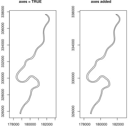
Despite the fact that computers have greater memory capacity than they used to,Rmay not be suitable for the analysis of massive data sets, because data being analysed is held in memory. Massive data sets may, for example come from satellite imagery, or detailed global coast line information. It is in such cases necessary to have some idea about data size and memory man-agement and requirements. Under such circumstances it is often still possible to useRas an analysis engine on part of the data sets. Smaller useful data sets can be obtained by selecting a certain region or by sub-sampling, aggregating or generalising the original data. Chapters 4 and 6 will give hints on how to do this. Spatial data are usually displayed on maps, where thex- andy-axes show the coordinate values, with the aspect ratio chosen such that a unit in x equals a unit in y. Another property of maps is that elements are added for reference purposes, such as coast lines, rivers, administrative boundaries, or even satellite images.

Display of spatial data inR is a challenge on its own, and is dealt with in Chap. 3. For many users, the graphical display of statistical data is among the most compelling reasons to useR, as maps are traditionally amongst the strongest graphics we know.

(26)

1.6 Applied Spatial Data Analysis

Statistical inference is concerned with drawing conclusions based on data and prior assumptions. The presence of a model of the data generating process may be more or less acknowledged in the analysis, but its reality will make itself felt sooner or later. The model may be manifest in the design of data collection, in the distributional assumptions employed, and in many other ways. A key in-sight is that observations in space cannot in general be assumed to be mutually independent, and that observations that are close to each other are likely to be similar (ceteris paribus). This spatial patterning – spatial autocorrelation – may be treated as useful information about unobserved inﬂuences, but it does challenge the application of methods of statistical inference that assume the mutual independence of observations.

Not infrequently, the prior assumptions are not made explicit, but are rather taken for granted as part of the research tradition of a particular scien-tific subdiscipline. Too little attention typically is paid to the assumptions, and too much to superficial differences; for example Venables and Ripley (2002, p. 428) comment on the difference between the covariance function and the semi-variogram in geostatistics, that ‘[m]uch heat and little light emerges from discussions of their comparison’.

To illustrate the kinds of debates that rage in disparate scientiﬁc com-munities analysing spatial data, we sketch two current issues: red herrings in geographical ecology and the interpretation of spatial autocorrelation in urban economics.

The red herring debate in geographical ecology was ignited by Lennon (2000), who claimed that substantive conclusions about the impact of envi-ronmental factors on, for example species richness had been undermined by not taking spatial autocorrelation into account. Diniz-Filho et al. (2003) replied challenging not only the interpretation of the problem in statistical terms, but pointing out that geographical ecology also involves the scale problem, that the inﬂuence of environmental factors is moderated by spatial scale.

They followed this up in a study in which the data were sub-sampled to attempt to isolate the scale problem. But they begin: ‘It is important to note that we do not present a formal evaluation of this issue using statistical theory. . ., our goal is to illustrate heuristically that the often presumed bias due to spatial autocorrelation in OLS regression does not apply to real data sets’ (Hawkins et al., 2007, p. 376).

(27)

methods themselves are unstable and generate conﬂicting results in real data, it makes no sense to claim that any particular method is always superior to any other’.

The urban economics debate is not as vigorous, but is of some practical interest, as it concerns the efficiency of services provided by local government. Revelli (2003) asks whether the spatial patterns observed in model residuals are a reaction to model misspecification, or do they signal the presence of substantive interaction between observations in space? In doing so, he reaches back to evocations of the same problem in the legacy literature of spatial statistics. As Cliff and Ord (1981, pp. 141–142) put it, ‘two adjacent super-markets will compete for trade, and yet their turnover will be a function of general factors such as the distribution of population and accessibility’. They stress that ‘the presence of spatial autocorrelation may be attributable either to trends in the data or to interactions; . . . [t]he choice of model must in-volve the scientific judgement of the investigator and careful testing of the assumptions’. When the fitted model is misspecified, it will be hard to draw meaningful conclusions, and the care advised by Cliff and Ord will be required. One way of testing the assumptions is through changes in the policy context over time, where a behavioural model predicts changes in spatial autocorrelation – if the policy changes, the level of spatial interaction should change (Bivand and Szymanski, 1997; Revelli, 2003). Alternatives include us-ing multiple levels in local government (Revelli, 2003), or different electoral settings, such as lame-duck administrations as controls (Bordignon et al., 2003). A recent careful study has used answers to a questionnaire survey to check whether interaction has occurred or not. It yields a clear finding that the observed spatial patterning in local government efficiency scores is related to the degree to which they compare their performance with that of other local government entities (Revelli and Tovmo, 2007).

This book will not provide explicit guidance on the choice of models, be-cause the judgement of researchers in diﬀerent scientiﬁc domains will vary. One aspect shared by both examples is that the participants stress the impor-tance of familiarity with the core literature of spatial statistics. It turns out that many of the insights found there remain fundamental, despite the pas-sage of time. Applied spatial data analysis seems to be an undertaking that, from time to time, requires the analyst to make use of this core literature.

Without attempting to be exhaustive in reviewing key books covering all the three acknowledged areas of spatial statistics – point processes, geostatis-tics, and areal data – we can make some choices. Bivand (2008, pp. 16–17) documents the enduring position of Ripley (1981)6 _{and Cliﬀ and Ord (1981)}

in terms of paper citations. Ripley (1988) supplements and extends the earlier work, and is worth careful attention. The comprehensive text by Cressie (1993) is referred to very widely; careful reading of the often very short passages of relevance to a research problem can be highly rewarding. Schabenberger and

(28)

Gotway (2005) cover much of the same material, incorporating advances made over the intervening period. Banerjee et al. (2004) show how the Bayesian ap-proach to statistics can be used in applied spatial data analysis.

Beyond the core statistical literature, many disciplines have their own tra-ditions, often collated in widely used textbooks. Public health and disease mapping are well provided for by Waller and Gotway (2004), as is ecology by Fortin and Dale (2005). O’Sullivan and Unwin (2003) cover similar topics from the point of view of geography and GIS. Like Banerjee et al. (2004), the disciplinary texts diﬀer from the core literature not only in the way theoretical material is presented, but also in the availability of the data sets used in the books for downloading and analysis. Haining (2003) is another book providing some data sets, and an interesting bridge to the use of Bayesian approaches in the geographies of health and crime. Despite its age, Bailey and Gatrell (1995) remains a good text, with support for its data sets inRpackages.

In an R News summary, Ripley (2001) said that one of the reasons for the relatively limited availability of spatial statistics functions in R at that time was the success of theS-PLUS™spatial statistics module (Kaluzny et al., 1998). Many of the methods for data handling and analysis are now available in Rcomplement and extend those in theS-PLUS™module. We also feel that the new packaging system inS-PLUS™constitutes an invitation, for instance to release packages likespforS-PLUS™– during the development of the package, it was tested regularly under both compute engines. Although the names of functions and arguments for spatial data analysis diﬀer betweenS-PLUS™and

R, users of theS-PLUS™spatial statistics module should have no diﬃculty in ‘ﬁnding their way around’ our presentation.

To summarise the approach to applied spatial data analysis adopted here, we can say that – as with the definition of geography as ‘what geographers do’ – applied spatial data analysis can best be understood by observing what practitioners do and how they do it. Since practitioners may choose to con-duct analyses in different ways, it becomes vital to keep attention on ‘how they do it’, which R facilitates, with its unrivalled closeness to both data and the implementation of methods. It is equally important to create and maintain bridges between communities of practitioners, be they innovative statisticians or dedicated field scientists, or (rarely) both in the same per-son. TheRSpatial community attempts to offer such opportunities, without necessarily prescribing or proscribing particular methods, and this approach will be reflected in this book.

1.7 R

Spatial Resources

(29)

spatial data analysis. Indeed, without contributions, advice, bug reports, and fruitful questions from users, very little would have been achieved. So before going on to present the structure of the book, we mention some of the more helpful online resources.

1.7.1 Online Resources

Since CRAN has grown to over 1,200 packages, ﬁnding resources is not sim-ple. One opportunity is to use the collection of ‘Task Views’ available on CRAN itself. One of these covers spatial data analysis, and is kept more-or-less up to date. Other task views may also be relevant. These web pages are intended to be very concise, but because they are linked to the resources listed, including packages on CRAN, they can be considered as a kind of ‘shop window’. By installing thectvpackage and executing the command in-stall.views("Spatial"), you will install almost all the contributed packages needed to reproduce the examples in this book (which may be downloaded from the book website).

The spatial task view is available on all CRAN mirrors, but may be ac-cessed directly;7 _{it provides a very concise summary of available contributed}

packages. It also specifically links two other resources, a mailing list dedicated to spatial data analysis withRand anR-Geo website. TheR-sig-geo mailing list was started in 2003 after sessions on spatial statistics at the Distributed Statistical Computing conference organised in Vienna earlier the same year. By late 2007, the mailing list was being used by over 800 members, off-loading some of the spatial topic traffic from the mainR-help mailing list. WhileR-help can see over 100 messages a day,R-sig-geo has moderate volume.

The archives of the mailing list are hosted in Zurich with the other R mailing list archives, and copies are held on Gmane and Nabble. This means that list traﬃc on an interesting thread can be accessed by general Internet search engines as well as theRSiteSearch()internalRsearch engine; a Google™ search onR gstat krigingpicks up list traﬃc easily.

The second linked resource is theR-Geo website, generously hosted since its inception by Luc Anselin, and is currently hosted at the Spatial Analy-sis Laboratory (SAL) in the Department of Geography at the University of Illinois, Urbana-Champaign. Because the site uses a content management sys-tem, it may be updated at will, but does not duplicate the CRAN task view. When users report news or issues, including installation issues, with packages, this is the site where postings will be made.

1.7.2 Layout of the Book

This book is divided into two basic parts, the ﬁrst presenting the shared R packages, functions, classes, and methods for handling spatial data. This part

(30)

is of interest to users who need to access and visualise spatial data, but who are not initially concerned with drawing conclusions from analysing spatial data per se. The second part showcases more specialised kinds of spatial data analysis, in which the relative position of observations in space may contribute to understanding the data generation process. This part is not an introduction to spatial statistics in itself, and should be read with relevant textbooks and papers referred to in the chapters.

Chapters 2 through 6 introduce spatial data handling inR. Readers need-ing to get to work quickly may choose to read Chap. 4 ﬁrst, and return to other chapters later to see how things work. Those who prefer to see the naked struc-ture ﬁrst before using it will read the chapters in sequence, probably omitting technical subsections. The functions, classes, and methods are indexed, and so navigation from one section to another should be feasible.

Chapter 2 discusses in detail the classes for spatial data inR, as imple-mented in the sp package, and Chap. 3 discusses a number of ways of visu-alising for spatial data. Chapter 4 explains how coordinate reference systems work in the sp representation of spatial data in R, how they can be deﬁned and how data can be transformed from one system to another, how spatial data can be imported into Ror exported fromRto GIS formats, and how R and the open source GRASS GIS are integrated. Chapter 5 covers methods for handling the classes deﬁned in Chap. 2, especially for combining and in-tegrating spatial data. Finally, Chap. 6 explains how the methods and classes introduced in Chap. 2 can be extended to suit one’s own needs.

If we use the classiﬁcation of Cressie (1993), we can introduce the applied spatial data analysis part of the book as follows: Chap. 7 covers the analysis of spatial point patterns, in which the relative position of points is compared with clustered, random, or regular generating processes. Chapter 8 presents the analysis of geostatistical data, with interpolation from values at observation points to prediction points. Chapters 9 and 10 deal with the statistical analysis of areal data, where the observed entities form a tessellation of the study area, and are often containers for data arising at other scales; Chap. 11 covers the special topic of disease mapping inR, and together they cover the analysis of lattice data, here termed areal data.

(31)

Classes for Spatial Data in

R

2.1 Introduction

Many disciplines have inﬂuenced the representation of spatial data, both in analogue and digital forms. Surveyors, navigators, and military and civil en-gineers reﬁned the fundamental concepts of mathematical geography, estab-lished often centuries ago by some of the founders of science, for example by al-Khw¯arizm¯ı. Digital representations came into being for practical reasons in computational geometry, in computer graphics and hardware-supported gam-ing, and in computer-assisted design and virtual reality. The use of spatial data as a business vehicle has been spurred in the early years of the present century by consumer broadband penetration and distributed server farms, with a prime example being Google Earth™.1_{There are often interactions}

be-tween the graphics hardware required and the services oﬀered, in particular for the fast rendering of scene views.

In addition, space and other airborne technologies have vastly increased the volumes and kinds of spatial data available. Remote sensing satellites continue to make great contributions to earth observation, with multi-spectral images supplementing visible wavelengths. The Shuttle Radar Topography Mission (SRTM) in February 2000 has provided elevation data for much of the earth. Other satellite-borne sensor technologies are now vital for timely storm warnings, amongst other things. These complement terrestrial networks monitoring, for example lightning strikes and the movement of precipitation systems by radar.

Surveying in the ﬁeld has largely been replaced by aerial photogram-metry, mapping using air photographs usually exposed in pairs of stereo images. Legacy aerial photogrammetry worked with analogue images, and many research laboratories and mapping agencies have large archives of air photographs with coverage beginning from the 1930s. These images can be scanned to provide a digital representation at chosen resolutions. While

(32)

satellite imagery usually contains metadata giving the scene frame – the sensor direction in relation to the earth at scan time – air photographs need to be registered to known ground control points.

These ground control points were ‘known’ from terrestrial triangulation, but could be in error. The introduction of Global Positioning System (GPS) satellites has made it possible to correct the positions of existing networks of ground control points. The availability of GPS receivers has also made it pos-sible for data capture in the ﬁeld to include accurate positional information in a known coordinate reference system. This is conditioned by the require-ment of direct line-of-sight to a suﬃcient number of satellites, not easy in mountain valleys or in city streets bounded by high buildings. Despite this limitation, around the world the introduction of earth observation satellites and revised ground control points have together caused breaks of series in published maps, to take advantage of the greater accuracy now available. This means that many older maps cannot be matched to freshly acquired position data without adjustment.

All of these sources of spatial data involve points, usually two real numbers representing position in a known coordinate reference system. It is possible to go beyond this simple basis by combining pairs of points to form line segments, combining line segments to form polylines, networks or polygons, or regular grid centres. Grids can be defined within a regular polygon, usually a rectangle, with given resolution – the size of the grid cells. All these definitions imply choices of what are known in geographical information systems (GIS) as data models, and these choices have most often been made for pragmatic reasons. All the choices also involve trade-offs between accuracy, feasibility, and cost.

(33)

many GIS packages do provide a 2.5D intermediate solution for viewing, by draping thematic layers, like land cover or a road network, over a digital el-evation model. In this case, however, there is no ‘depth’ in the data model, as we can see when a road tunnel route is draped over the mountain it goes through.

2.2 Classes and Methods in

R

In Chap. 1, we describedRas a language and environment for data analysis. Although this is not the place to give an extended introduction toR,2 _{it will}

be useful to highlight some of its features (see also Braun and Murdoch, 2007, for an up-to-date introduction). In this book, we will be quotingRcommands in the text, showing which commands a user could give, and how the non-graphical output might be represented when printed to the console.

Of course,Rcan be used as a calculator to carry out simple tasks, where no values are assigned to variables, and where the results are shown without being saved, such as the area of a circle of radius 10:

> pi * 10^2

[1] 314.1593

Luckily,πis a built-in constant inRcalledpi, and so entering a rounded version is not needed. So this looks like a calculator, but appearances mislead. The ﬁrst misleading impression is that the arithmetic is simply being ‘done’, while in fact it is being translated (parsed) into functions (operators) with arguments ﬁrst, and then evaluated:

> "*"(pi, "^"(10, 2))

[1] 314.1593

When the operators or functions permit, vectors of values may be used as readily as scalar values (which are vectors of unit length) — here the‘:’

operator is used to generate an integer sequence of values: > pi * (1:10)^2

[1] 3.141593 12.566371 28.274334 50.265482 78.539816 113.097336 [7] 153.938040 201.061930 254.469005 314.159265

The second misapprehension is that what is printed to the console is the ‘result’, when it is actually the outcome of applying the appropriate print

method for the class of the ‘result’, with default arguments. If we store the value returned for the area of our circle in variable x using the assignment operator<-, we can printxwith the default number of digits, or with more if

2_{Free documentation, including the very useful ‘An Introduction to}_R_{’ (Venables}

(34)

we so please. Just typing the variable name at the interactive prompt invokes the appropriate print method, but we can also pass it to the print method explicitly:

> x <- pi * 10^2 > x

[1] 314.1593

> print(x)

[1] 314.1593

> print(x, digits = 12)

[1] 314.159265359

We can say that the variablexcontains an object of a particular class, in this case:

> class(x)

[1] "numeric"

> typeof(x)

[1] "double"

where typeof returns the storage mode of the object in variablex. It is the class of the object that determines the method that will be used to handle it; if there is no speciﬁc method for that class, it may be passed to a default method. These methods are also known as generic functions, often including at least print,plot, andsummary methods. In the case of theprint method,

numericis not provided for explicitly, and so the default method is used. The

plot method, as its name suggests, will use the current graphics device to make a visual display of the object, dispatching to a speciﬁc method for the object class if provided. In comparison with the print method, the summary

method provides a qualiﬁed view of the data, highlighting the key features of the object.

When the S language was first introduced, it did not use class/method mechanisms at all. They were introduced in Chambers and Hastie (1992) and S version 3, in a form that is known asS3classes or old-style classes. These classes were not formally defined, and ‘just grew’; the vast majority of objects returned by model fitting functions belong to old-style classes. Using a non-spatial example from the standard data setcars, we can see that it is an object of classdata.frame, stored in alist, which is a vector whose components can be arbitrary objects;data.framehas both names and summary methods:

> class(cars)

(35)

> typeof(cars)

[1] "list"

> names(cars)

[1] "speed" "dist"

> summary(cars)

speed dist

Min. : 4.0 Min. : 2.00 1st Qu.:12.0 1st Qu.: 26.00 Median :15.0 Median : 36.00 Mean :15.4 Mean : 42.98 3rd Qu.:19.0 3rd Qu.: 56.00 Max. :25.0 Max. :120.00

The data.frame contains two variables, one recording the speed of the observed cars in mph, the other the stopping distance measured in feet – the observations were made in the 1920s. When uncertain about the structure of something in ourRworkspace, revealed for example by using thelsfunction for listing the contents of the workspace, thestr3method often gives a clear digest, including the size and class:

> str(cars)

'data.frame': 50 obs. of 2 variables: $ speed:num 4 4 7 7 8 ...

$ dist :num 2 10 4 22 16 ...

Data frames are containers for data used everywhere inSsince their full introduction in Chambers and Hastie (1992, pp. 45–94). Recent and shorter introductions to data frames are given by Crawley (2005, pp. 15–22), Crawley (2007, pp. 107–133), and Dalgaard (2002, pp. 18–19) and in the online doc-umentation (Venables et al., 2008, pp. 27–29 in the R 2.6.2 release). Data frames view the data as a rectangle of rows of observations on columns of val-ues of variables of interest. The representation of the valval-ues of the variables of interest can include integer and ﬂoating point numeric types, logical, char-acter, and derived classes. One very useful derived class is the factor, which is represented as integers pointing to character levels, such as ‘forest’ or ‘arable’. Printed, the values look like character values, but are not – when

a data frame is created, all character variables included in it are converted to factor by default. Data frames also have unique row names, represented as an integer or character vector or as an internal mechanism to signal that

(36)

the sequence from 1 to the number of rows in the data frame are used. The

row.namesfunction is used to access and assign data frame row names.

One of the fundamental abstractions used inRis theformulaintroduced in Chambers and Hastie (1992, pp. 13–44) – an online summary may be found in Venables et al. (2008, pp. 50–52 in the R 2.6.2 release). The abstraction is intended to make statistical modelling as natural and expressive as pos-sible, permitting the analyst to focus on the substantive problem at hand. Because the formula abstraction is used in very many contexts, it is worth some attention. Aformula is most often two-sided, with a response variable to the left of the∼(tilde) operator, and in this case a determining variable on the right:

> class(dist ~ speed)

[1] "formula"

These objects are typically used as the first argument to model fitting func-tions, such as lm, which is used to fit linear models. They will usually be

accompanied by a data argument, indicating where the variables are to be found:

> lm(dist ~ speed, data = cars)

Call:

lm(formula = dist ~ speed, data = cars)

Coefficients:

(Intercept) speed

-17.579 3.932

This is a simple example, but very much more can be done with theformula

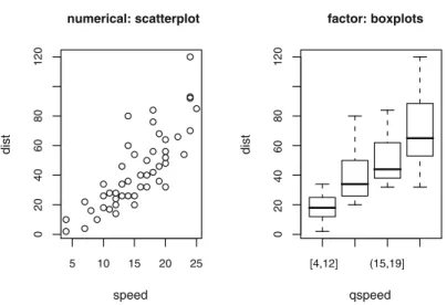
abstraction. If we create a factor for the speed variable by cutting it at its quartiles, we can contrast how theplot method displays the relationship be-tween two numerical variables and a numerical variable and a factor (shown in Fig. 2.1):

> cars$qspeed <- cut(cars$speed, breaks = quantile(cars$speed), + include.lowest = TRUE)

> is.factor(cars$qspeed)

[1] TRUE

> plot(dist ~ speed, data = cars) > plot(dist ~ qspeed, data = cars)

(37)

5 10 15 20 25

0

2

0

4

0

6

0

8

0

120

numerical: scatterplot

speed

dist

[4,12] (15,19]

0

2

0

4

0

6

0

8

0

120

factor: boxplots

qspeed

dist

Fig. 2.1. Plot methods for a formula with numerical (left panel) and factor (right panel) right-hand side variables

> lm(dist ~ qspeed, data = cars)

Call:

lm(formula = dist ~ qspeed, data = cars)

Coefficients:

(Intercept) qspeed(12,15] qspeed(15,19] qspeed(19,25]

18.20 21.98 31.97 51.13

Variables in the formula may also be transformed in diﬀerent ways, for

ex-ample usinglog. The formula is carried through into the object returned by

model ﬁtting functions to be used for prediction from new data provided in a

data.framewith the same column names as the right-hand side variables, and

the same level names if the variable is a factor.

New-style (S4) classes were introduced in the S language at release 4, and in Chambers (1998), and are described by Venables and Ripley (2000, pp. 75–121), and in subsequent documentation installed with R.4 _Old-style

classes are most often simply lists with attributes; they are not defined for-mally. Although users usually do not change values inside old-style classes, there is nothing to stop them doing so, for example changing the representa-tion of coordinates from floating point to integer numbers. This means that functions need to check, among other things, whether components of a class exist, and whether they are represented correctly, before they can be handled. The central advantage of new-style classes is that they have formal definitions

4_{There is little instructional material online, although this use}_R _conference

(38)

that specify the name and type of the components, called slots, that they contain. This simpliﬁes the writing, maintenance, and use of the classes, be-cause their format is known from the deﬁnition. For a further discussion of programming for classes and methods, see Sect. 6.1.

Because the classes provided by thesp package are new-style classes, we will be seeing how such classes work in practice below. In particular, we will be referring to the slots in class definitions; slots are specified in the definition as the representation of what the class contains. Many methods are written for the classes to be introduced in the remainder of this chapter, in particular coercion methods for changing the way an object is represented from one class to another. New-style classes can also check the validity of objects being cre-ated, for example to stop the user from filling slots with data that do not conform to the definition.

2.3 Spatial

Objects

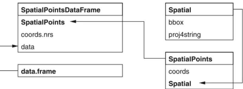
The foundation class is the Spatial class, with just two slots. The first is a bounding box, a matrix of numerical coordinates with column namesc(‘min’, ‘max’), and at least two rows, with the first row eastings (x-axis) and the second northings (y-axis). Most often the bounding box is generated auto-matically from the data in subclasses of Spatial. The second is a CRS class object defining the coordinate reference system, and may be set to ‘missing’, represented by NA in R, by CRS(as.character(NA)), its default value. Oper-ations on Spatial* objects should update or copy these values to the new

Spatial* objects being created. We can usegetClass to return the complete deﬁnition of a class, including its slot names and the types of their contents: > library(sp)

> getClass("Spatial")

Slots:

Name: bbox proj4string

Class: matrix CRS

Known Subclasses:

Class "SpatialPoints", directly Class "SpatialLines", directly Class "SpatialPolygons", directly

Class "SpatialPointsDataFrame", by class "SpatialPoints", distance 2 Class "SpatialPixels", by class "SpatialPoints", distance 2

Class "SpatialGrid", by class "SpatialPoints", distance 3

Class "SpatialPixelsDataFrame", by class "SpatialPoints", distance 3 Class "SpatialGridDataFrame", by class "SpatialPoints", distance 4 Class "SpatialLinesDataFrame", by class "SpatialLines", distance 2 Class "SpatialPolygonsDataFrame", by class "SpatialPolygons",

(39)

As we see, getClass also returns known subclasses, showing the classes that

include the Spatial class in their deﬁnitions. This also shows where we are

going in this chapter, moving from the foundation class to richer represen-tations. But we should introduce the coordinate reference system (CRS) class very brieﬂy; we will return to its description in Chap. 4.

> getClass("CRS")

Slots:

Name: projargs Class: character

The class has a character string as its only slot value, which may be a missing value. If it is not missing, it should be a PROJ.4-format string describing the projection (more details are given in Sect. 4.1.2). For geographical coordinates, the simplest such string is"+proj=longlat", using"longlat", which also shows that eastings always go before northings inspclasses. Let us build a simple

Spatialobject from a bounding box matrix, and a missing coordinate reference system:

> m <- matrix(c(0, 0, 1, 1), ncol = 2, dimnames = list(NULL, + c("min", "max")))

> crs <- CRS(projargs = as.character(NA)) > crs

CRS arguments: NA

> S <- Spatial(bbox = m, proj4string = crs) > S

An object of class "Spatial" Slot "bbox":

min max [1,] 0 1 [2,] 0 1

Slot "proj4string": CRS arguments: NA

We could have used new methods to create the objects, but prefer to use helper functions with the same names as the classes that they instantiate. If the object is known not to be projected, a sanity check is carried out on the coordinate range (which here exceeds the feasible range for geographical coordinates):

> Spatial(matrix(c(350, 85, 370, 95), ncol = 2, dimnames = list(NULL, + c("min", "max"))), proj4string = CRS("+longlat"))